Classical analog for dispersion cancellation of entangled photons with local detection

Abstract

Energy-time entangled photon pairs remain tightly correlated in time when the photons are passed through equal magnitude, but opposite in sign, dispersion. A recent experimental demonstration has observed this effect on ultrafast time-scales using second-harmonic generation of the photon pairs. However, the experimental signature of this effect does not require energy-time entanglement. Here, we demonstrate a directly analogue to this effect in narrow-band second harmonic generation of a pair of classical laser pulses under similar conditions. Perfect cancellation is observed for fs pulses with dispersion as large as $850$ fs², comparable to the quantum result, but with an $10^{13}$-fold improvement in signal brightness.

Introduction – Ultrafast pulses of light are indispensable tools at the heart of technologies as diverse as time-resolved spectroscopy, fusion energy, surgery, micro-machining, and medical imaging diels06 . These pulses require a very large bandwidth of light, all locked together in phase, to support them. This makes the pulses very susceptible to the effects of dispersion, the change of the group velocity of the light with respect to frequency. Dispersion slows some of the frequency components of the pulse relative to others and spreads the pulse in time, an effect that becomes more pronounced with larger bandwidth. If the timing information carried by the pulse is critical to the application, such as clock synchronization giovannetti01 or interferometry, this is clearly detrimental.

In 1992, two seminal papers steinberg92 ; franson92 showed that energy-time entangled photons exhibit an inherent robustness against dispersion, in two very different scenarios. The first scenario considered the Hong-Ou-Mandel two-photon interferometer with unbalanced dispersion, such as that from an extra piece of glass, in one arm. The Hong-Ou-Mandel interference dip Hong87 , whose width is equal to the coherence length of the photons, is completely unaffected by all even orders of dispersion steinberg92b ; resch09footnote ; resch09 . This effect has been shown to have classical analogues erkmen06 ; banaszek07 ; resch07 ; kaltenbaek08 ; legouet10 .

The second scenario was considered by Franson franson92 . If a pair of transform-limited classical light pulses is sent to different detectors, then any quadratic dispersion during the propagation hurts their temporal correlation. Recently it was shown that the effect on the correlation for classical pulses can be expressed as an inequality wasak10 ,

$$\langle\Delta\tau_{F}^{2}\rangle\geq\langle\Delta\tau^{2}\rangle+\frac{(2\beta)^{2}}{\langle\Delta\tau^{2}\rangle}$$ (1)

where $\langle\Delta\tau_{F}^{2}\rangle$ is the final variance in the time difference of the detection signals, $\langle\Delta\tau^{2}\rangle$ is the initial variance, and $\beta$ characterizes the dispersion which applies a quadratic frequency dependent phase $\phi(\omega)=\beta(\omega-\omega_{0})^{2}$ about some centre frequency $\omega_{0}$. Franson calculated that if, instead, energy-time entangled photon pairs were sent to the different detectors, as shown in Fig. 1(a), the photon pairs remained tightly coincident in time when one photon passed through positive dispersion and the other passed through equal magnitude negative dispersion franson92 . Thus Eq. 1, can be violated for entangled photons.

In order to observe this effect, one needs to introduce dispersion significant on the timescale of the detector response. Direct detection of dispersion cancellation using single-photon counters and coincidence detection requires large dispersion on the  ns scale, as was achieved in Refs. brendel98 ; baek09 . A very recent experiment by O’Donnell odonnell11 , probes dispersion cancellation with femtosecond resolution using second-harmonic generation of photon pairs followed by photon counting of the up-converted beam as an ultrafast coincidence detector dayan05 ; odonnell09 . (The short coincidence window originates from the speed of the nonlinear process and persists even when the detector is orders of magnitude slower). The second-harmonic generation signal originates from simultaneously arriving photons, but by varying an optical delay, $\tau$, one can measure temporal correlations with a time offset odonnell09 . Unlike the prior experiments which follow Franson’s original proposal franson92 by sending the photons to different detectors (as in Fig. 1(a)), O’Donnell’s experiment necessarily recombines the photons for the second-harmonic process (Fig 1(b)), i.e., it uses local detection. It has been argued that dispersion cancellation cannot be observed with only classical resources in the original, nonlocal, scenario franson92 ; wasak10 , albeit with a fair amount of recent discussion torrescompany09 ; franson09 ; shapiro10 ; franson10 ; however, with local detection these arguments no longer apply.

One approach that has proven fruitful for developing classical analogues of quantum technologies bennink02 ; ferri05 ; hemmer06 ; bentley04 ; torres11 is that of time reversal resch07b ; kaltenbaek08 ; kaltenbaek09 ; lavoie09 . Under this transformation down-conversion, which is exclusively quantum mechanical, can be replaced by second-harmonic generation, which is a classical process. In the present work, we show that the same signal observed in O’Donnell’s experiment with entangled photons can, in fact, be observed in a completely classical experiment. Schematically, our setup is shown in Fig. 1(c) where it can be viewed as the time-reverse of Franson’s original proposal, Fig. 1(a). A pair of time-correlated short laser pulses are sent through two dispersive media. The resulting pulses undergo fast second-harmonic generation and photons of frequency $2\omega_{0}$ are detected using a standard single-photon counter.

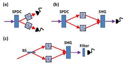
Figure 1: (a) In Franson’s proposal franson92 , a narrowband laser photon produces a pair of energy-time entangled photons via spontaneous parametric down-conversion (SPDC). Each photon passes through different media characterized by second-order dispersion coefficient, $\beta$. Fast photon counters register the photon pairs and allow to determine the average time difference in detection, $\langle\Delta\tau\rangle$. For perfectly energy-time entangled photons with $\beta_{2}=-\beta_{1}$, the effect of the dispersions cancel, and the pairs exhibit no additional broadening. (b) In O’Donnell’s experiment odonnell11 , the photon counters and coincidence detection are replaced by second-harmonic generation which allows to probe dispersion effects on the  fs timescale. (c) In the present work, we use a pair of classical laser pulses instead of entangled photons. We use second-harmonic generation, as in (b), but add narrow spectral filtering before detection of the second harmonic light. The detected light has the same temporal characteristics of that in (b), including dispersion cancellation.

Theory – In the literature, Franson dispersion cancellation has been considered for the case of perfect energy-time entanglement. We first reanalyze this effect using a physically-motivated model with variable energy-time entanglement. We consider the two-mode state,

$$|\psi\rangle\sim\iint d\omega_{1}d\omega_{2}f(\omega_{1},\omega_{2})|\omega_{1}\rangle|\omega_{2}\rangle,$$ (2)

where we model the spectral function as in Ref. resch09 ,

$$f(\omega_{1},\omega_{2})=e^{-\frac{(\omega_{1}-\omega_{0})^{2}}{2\sigma^{2}}}e^{-\frac{(\omega_{2}-\omega_{0})^{2}}{2\sigma^{2}}}e^{-\frac{(\omega_{1}+\omega_{2}-2\omega 0)^{2}}{2\sigma_{c}^{2}}}$$ (3)

with the spectrum of each photon given by a Gaussian distribution centered at $\omega_{0}$ with rms width $\sigma$. Here, $\sigma_{c}$ describes the strength of the energy correlation between the modes – for down-conversion sources, this parameter is given by the pump bandwidth. If $\sigma_{c}\gg\sigma$, $f(\omega_{1},\omega_{2})$ factorizes and the state is separable while if $\sigma_{c}\rightarrow 0$ then the photons are perfectly energy anticorrelated and we obtain the perfect energy-time entangled state. Using the same approach as in franson92 , we calculate the probability of detecting one photon at time, $t_{1}$, and another at time $t_{2}$, using the correlation function,

$$P\propto\langle\hat{E}_{1}^{-}(x_{1},t_{1})\hat{E}_{2}^{-}(x_{2},t_{2})\hat{E}_{1}^{+}(x_{1},t_{1})\hat{E}_{2}^{+}(x_{2},t_{2})\rangle,$$ (4)

where the positive frequency electric field operator is $\hat{E}_{i}^{+}(x,t)=i\sum_{\omega}\left(\frac{\hbar\omega}{2\varepsilon_{0}V}\right)^{1/2}e^{i(kx-\omega t)}\hat{a_{i}}(\omega)$ and $\hat{E}_{i}^{-}=(\hat{E}_{i}^{+})^{\dagger}$ loudon83 . As in Ref. franson92 we assume that the bandwidth is small so we can remove $\sqrt{\omega}$ dependence from the summation. We characterize the quadratic dispersion of each photon using the coefficient $\beta=\frac{1}{2}\frac{d^{2}k}{d\omega^{2}}L$, where $L$ is the length of the dispersive region, so that $\phi(\omega)=k(\omega)L=\beta(\omega-\omega_{0})^{2}$. With this simplifying assumption and the condition considered in Ref. franson92 that $\beta_{2}=-\beta_{1}$, the coincidence probability is,

$$P(t_{1},t_{2})\propto\exp\left[{-\frac{(t_{1}-t_{2})^{2}\sigma^{4}+(t_{1}^{2}+t_{2}^{2})\sigma^{2}\sigma_{c}^{2}}{2\sigma^{2}+\sigma_{c}^{2}+4\beta_{1}^{2}\sigma^{4}\sigma_{c}^{2}}}\right].$$ (5)

From this distribution we calculate the variance in the time difference of detections, $\Delta\tau_{Q}^{2}=\Delta(t_{1}-t_{2})^{2}$,

$$\Delta\tau_{Q}^{2}=\frac{1}{\sigma^{2}}\left(1+\frac{4\beta_{1}^{2}\sigma^{4}\sigma_{c}^{2}}{2\sigma^{2}+\sigma_{c}^{2}}\right).$$ (6)

This allows us to recover key results of Ref. franson92 in different limits. In the limit of perfect energy-time entanglement, $\sigma_{c}\rightarrow 0$, we have perfect dispersion cancellation since $\Delta\tau_{Q}^{2}=\frac{1}{\sigma^{2}}$ and the dispersion does not reduce the temporal correlation at all, clearly violating the inequality in Eq. 1. In the opposite limit where there is no energy-time entanglement, $\sigma_{c}\rightarrow\infty$, we have $\Delta\tau_{Q}^{2}=\frac{1}{\sigma^{2}}(1+4\beta_{1}^{2}\sigma^{4})$, i.e., the photon temporal correlations are as susceptible to dispersion as classical pulses (cf. Ref. (franson92, , Eq. 20)) and cannot violate Eq. 1.

Although infinitely narrow pump bandwidth SPDC, i.e, $\sigma_{c}\rightarrow 0$, is unphysical, it is experimentally straightforward to have a pump bandwidth orders of magnitude narrower than that of the photons, $\sigma_{c}\ll\sigma$. In this case,

$$\Delta\tau_{Q}^{2}\approx\frac{1}{\sigma^{2}}\left(1+2\beta_{1}^{2}\sigma^{2}\sigma_{c}^{2}\right).$$ (7)

Comparing this to the completely separable case we see that the effective bandwidth $\sigma$ is lowered approximately to the geometric average of the pump and photon bandwidth, $\sqrt{\sigma\sigma_{c}}$. Since this effective bandwidth is much smaller, the effect of dispersion on the temporal correlation is significantly reduced.

We now compare this quantum mechanical situation to the classical scenario shown in Fig. 1(c). We model a transform-limited classical pulse using its complex electric field amplitude,

$$E(\omega)\propto e^{-\frac{(\omega-\omega_{0})^{2}}{2\sigma^{2}}}.$$ (8)

We approximate the SHG of a fast nonresonant three-wave mixing interaction as,

$$E_{SHG}(\omega)\propto\int E_{1}(\omega^{\prime})E_{2}(\omega-\omega^{\prime})d\omega^{\prime},$$ (9)

which holds for a fast nonlinearity within a relatively narrow frequency band (the latter approximation is similar to removing the $\sqrt{\omega}$ outside the summation in the electric field operator). Including the effect of dispersion in both arms and a time delay, $\tau$, on one of the pulses, the second-harmonic amplitude at frequency $\omega$ is,

$$E_{SHG}(\omega) \propto$$

$$\int E_{1}(\omega^{\prime})e^{i\beta_{1}(\omega^{\prime}-\omega_{0})^{2}}e^{-i\omega^{\prime}\tau}E_{2}(\omega-\omega^{\prime})e^{i\beta_{2}(\omega-\omega^{\prime}-\omega_{0})^{2}}d\omega^{\prime}.$$

The intensity of the light is then measured at a single frequency using a monochromator with a finite frequency resolution, $\sigma_{s}$. We model the monochromator response using the resolution function $S(\omega)=e^{-\frac{(\omega-2\omega_{0})}{2\sigma_{s}^{2}}}$, so that the detected signal is

$$I\propto\int S(\omega)I(\omega)d\omega.$$ (11)

We calculate the expected signal, under the condition $\beta_{2}=-\beta_{1}$, as a function of the time delay, $\tau$, to be

$$I(\tau)\propto\exp\left[-\frac{\sigma^{2}(\sigma^{2}+\sigma_{s}^{2})\tau^{2}}{2(\sigma^{2}+\sigma_{s}^{2}+4\beta_{1}^{2}\sigma^{4}\sigma_{s}^{2})}\right].$$ (12)

From this expression we can compute the variance,

$$\Delta\tau_{C}^{2}=\frac{1}{\sigma^{2}}\left(1+\frac{4\beta_{1}^{2}\sigma^{4}\sigma_{s}^{2}}{\sigma^{2}+\sigma_{s}^{2}}\right).$$ (13)

Our expressions for the variances of quantum and classical signals, Eqs. 6 and 13, are remarkably similar. Both signals show perfect dispersion cancellation in the limits of $\sigma_{c}$ or $\sigma_{s}\rightarrow 0$. Thus the pump bandwidth in the quantum case plays the same role as spectrometer resolution in the classical case. These will, in practice, put constraints on the amount of dispersion cancellation possible. Assuming $\sigma_{c(s)}\ll\sigma$, then the condition $\beta\sigma_{c(s)}\sigma<1$ is still required for significant dispersion cancellation.

Experiment–Our experimental setup is depicted in Fig. 2. Light from a pulsed titanium:sapphire laser (KMLabs Griffin-10, centre wavelength $807\,\mbox{nm}$), passes through a 4-F pulse shaping apparatus containing a spatial light modulator (SLM) (CRi 640 pixel, dual mask) weiner00 . The pulse shaper is used to recompress the pulses from the laser and also to apply the negative quadratic dispersion. After exiting the pulse shaper, the light is split into two paths using a 50/50 non-polarizing, low-dispersion beamsplitter. We can introduce positive dispersion into one of the arms using BK7 glass plates. The two beams are then redirected and focused together onto a 2-mm thick bismuth borate (BiBO) crystal cut for second-harmonic generation. The upconverted light, which had an average power of $30\,\mbox{mW}$ when no additional dispersion was introduced, is filtered from the remaining fundamental, passed through a monochromator (at wavelength $404\,\mbox{nm}$) with 0.02 nm FWHM resolution, and its intensity measured by a photomultiplier tube (PMT). Using this monochromator resolution and the bandwidth of the laser, we expect that dispersion cancellation should persist for dispersion up to $\beta<1/\sigma_{c(s)}\sigma\approx 7\times 10^{4}\,\mbox{fs}^{2}$ according to the criterion derived in the previous section.

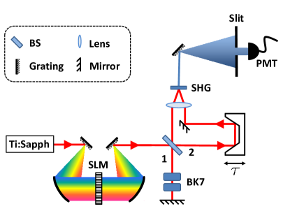
Figure 2: Experimental setup. The pulsed laser light from the Ti:Sapph is sent through a 4-F pulse shaper consisting of two 1200 l/mm gratings, two curved mirrors and a 640 pixel spatial light modulator (SLM). Subsequently, the beams are separated into two arms by a 50/50 beamsplitter (BS). In our experiment, positive dispersion in the sample arm (mode 1) can be introduced using two pieces of BK7 glass ($19.33\pm 0.03\,\mbox{mm}$ each), while the reference arm features an adjustable path delay, $\tau$. To observe dispersion cancellation, the beams are focused by a 75 mm achromatic lens onto a 2 mm BiBO nonlinear crystal and the upconverted light is spectrally filtered by a grating and a slit before detection by a PMT.

We first compensated quadratic and cubic dispersion using the pulse shaper to create a transform-limited laser pulse. Note that at this point there is no dispersion introduced in arm 1 of the interferometer. We recorded the second-harmonic intensity through our monochromator as a function of delay position, as shown in Fig. 3(a). The data show a sharply peaked signal with width $21.7\,\mbox{fs}$ FWHM. This is in good agreement with the estimated signal width of $20\,\mbox{fs}$ for the measured FWHM bandwidth of our laser’s electric field spectrum ($\Delta\lambda=97\,\mbox{nm}$). We measured the amount of positive dispersion introduced by two identical pieces of BK7 glass, totalling $38.65\pm 0.06\,\mbox{mm}$ thickness, by inserting it in the path before the beamsplitter, and applying negative quadratic dispersion with the SLM until we achieved the same width in our SHG signal as in Fig. 3(a). The dispersion of the glass was thus measured to be $\beta=850\,\mbox{fs}^{2}$ in good agreement with the theoretical value of $\beta=851\pm 1\,\mbox{fs}^{2}$, calculated from Sellmeier coefficients.

Using the transform-limited pulses, we inserted one piece of glass into the arm 1 of the interferometer. The light in that arm makes two passes through the glass and thus experiences $850\,\mbox{fs}^{2}$ of dispersion. The second-harmonic intensity as a function of delay is shown in Fig. 3(b), where the signal is significantly broadened to $172.7$ fs. Next, we used the SLM to apply $-850\,\mbox{fs}^{2}$ of dispersion, which compensates the glass in arm 1, but leaves the beam in arm 2 with negative dispersion. The second-harmonic signal in this case is shown in Fig. 3(c) and shows a similar level of broadening to $176.4$ fs. As expected here, and in agreement with the quantum theory and experiment franson92 ; odonnell11 , dispersion in either arm leads to broadening of the temporal correlation.

Finally, leaving the SLM applying $-850\,\mbox{fs}^{2}$ we added a second piece of glass to arm 1, so that the cumulative effect of the SLM and two pieces of glass resulted in $+850\,\mbox{fs}^{2}$ of net dispersion for that arm, while the beam in arm 2 remained at $-850\,\mbox{fs}^{2}$. The second-harmonic data for this case is shown in Fig. 3(d). The measured width is $21.9\,\mbox{fs}^{2}$, unchanged from the zero dispersion case. This is our classical analogue to dispersion cancellation with local detection. Our measured signal of $750\,\mu\mbox{W}$ corresponds to a photon flux of $6\times 10^{16}s^{-1}$, an $10^{13}$ increase over the signal reported in Ref. odonnell11 .

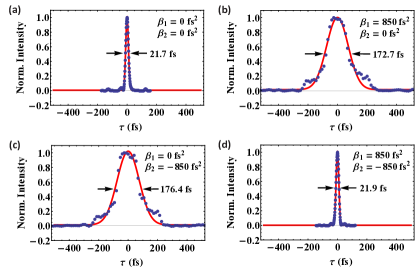
Figure 3: Experimental data. The normalized intensity of the upconverted light is shown as a function of the temporal delay, $\Delta\tau$. (a) shows the dispersion-free case with a nearly Fourier-limited signal width ($21.7$fs). This is in stark contrast to the cases where dispersion of (b) $\beta=850$ fs² is added to arm 1 or (c) $\beta=-850$ fs² is added to arm 2, where the signals broaden significantly to 172.7 fs and 176.4 fs, respectively. However, adding positive dispersion of $\beta=850$ fs² to arm 1 and negative dispersion $\beta=-850$ fs² to arm 2 yields the signal shown in (d) with a measured width of $21.9$  fs. In this last case, we show the dispersion is cancelled in direct analogy with the quantum effect.

Conclusion – Franson dispersion cancellation reveals a curious robustness of temporal correlations in energy-time entanglement. However, once local detection is introduced, it is straightforward to observe dispersion cancellation in a classical experiment, with signals 13 orders of magnitude higher than in a recent state of the art quantum experiment odonnell11 . It is interesting to consider whether applications in interferometry or clock synchronization could make use of the effect with the local detection constraint, as their performance would dramatically improve from the increase in signal alone. Regardless, our understanding of both theories is improved by exploring the limits of classical physics to emulate quantum mechanical effects.

Acknowledgements – We thank K. Shalm and R. Kaltenbaek for valuable discussions and are grateful for financial support from Ontario Ministry of Research and Innovation ERA, QuantumWorks, NSERC, OCE, Industry Canada and CFI. R.P. acknowledges support by MRI and the Austrian Science Fund (FWF).

References

- (1) J.C. Diels and W. Rudolph, Ultrashort laser pulse phenomena: Fundamentals, techniques, and applications on the femtosecond timescale, 2nd ed. (Academic Press, Burlington, USA 2006).
- (2) V. Giovannetti, S. Lloyd, L. Maccone, and F.N.C. Wong, Phys. Rev. Lett. 87, 117902 (2001).
- (3) A.M. Steinberg, P.G. Kwiat, and R.Y. Chiao, Phys. Rev. Lett. 68, 2421 (1992).
- (4) J.D. Franson, Phys. Rev. A 45, 3126 (1992).
- (5) C. K. Hong, Z. Y. Ou, and L. Mandel, Phys. Rev. Lett 59, 2044 (1987).
- (6) A.M. Steinberg, P.G. Kwiat, and R.Y. Chiao, Phys. Rev. A 45, 6659 (1992).
- (7) Even-order dispersion cancellation in the Hong-Ou-Mandel interferometer is ideal only when the energy-time entanglement is perfect. Once finite correlations are considered, the degree of cancellation is limited. However, with reasonable experimental parameters the impact on the interferometer signal under considerable amounts of dispersion can be dramatically reduced resch09 .
- (8) K.J. Resch, R. Kaltenbaek, J. Lavoie, and D.N. Biggerstaff, Proc. SPIE 7465, 74650N (2009).
- (9) B.I. Erkmen and J.H. Shapiro, Phys. Rev. A 74, 041601 (2006).
- (10) K. Banaszek, A.S. Radunsky, and I.A. Walmsley, Opt. Commun. 269, 152 155 (2007).
- (11) K.J. Resch, P. Puvanathasan, J.S. Lundeen, M.W. Mitchell, and K. Bizheva, Optics Express 15, 8797 (2007).
- (12) R. Kaltenbaek, J. Lavoie, D.N. Biggerstaff, and K.J. Resch, Nat. Phys. 4, 864 (2008).
- (13) J. Le Gouët, D.Venkatraman, F.N.C. Wong, and J.H. Shapiro, Opt. Lett. 35, 1001 (2010).
- (14) T. Wasak, P. Szańkowski, W. Wasilewski, and K. Banaszek, Phys. Rev. A 82, 052120 (2010).
- (15) J. Brendel, H. Zbinden, and N. Gisin, Optics Communications 151, 35 (1998).
- (16) S.-Y. Baek, Y.-W.Cho, and Y.-H. Kim, Opt. Express 17, 19241 (2009).
- (17) K.A. O’Donnell, Phys. Rev. Lett 106, 063601 (2011).
- (18) B. Dayan, A. Pe’er, A.A. Friesem, and Y. Silberberg, Phys. Rev. Lett. 94, 043602 (2005).
- (19) K.A. O’Donnell, A.B. U’Ren, Phys. Rev. Lett. 103, 123602 (2009).
- (20) V. Torres-Company, H. Lajunen, and A.T. Friberg, New J. Phys. 11, 063041 (2009).
- (21) J.D. Franson, Phys. Rev. A 80, 032119 (2009).
- (22) J.H. Shapiro, Phys. Rev. A 81, 023824 (2010).
- (23) J.D. Franson, Phys. Rev. A 81, 023825 (2010).
- (24) R.S. Bennink, S.J. Bentley, and R.W. Boyd, Phys. Rev. Lett. 89, 113601 (2002).
- (25) F. Ferri et al., Phys. Rev. Lett. 94, 183602 (2005).
- (26) P.R. Hemmer, A. Muthukrishnan, M.O. Scully, and M.S. Zubairy, Phys. Rev. Lett. 96, 163603 (2006).
- (27) S. Bentley and R. Boyd, Opt. Express 12, 5735 (2004).
- (28) V. Torres-Company, A. Valencia, M. Hendrych, and J. P. Torres, Phys. Rev. A 83, 023824 (2011).
- (29) K.J. Resch, et al. Phys. Rev. Lett. 98, 223601 (2007).
- (30) R. Kaltenbaek, J. Lavoie, and K.J. Resch, Phys. Rev. Lett. 102, 243601 (2009).
- (31) J. Lavoie, R. Kaltenbaek, and K.J. Resch, Opt. Express 17, 3818 (2009).
- (32) R. Loudon, The quantum theory of light, 2nd ed. (Oxford University Press, Oxford, UK 1983)
- (33) A.M. Weiner, Rev. Sci. Inst. 71, 1929 (2000)