Stability of Brans-Dicke thin shell wormholes

Abstract

Recently, a class of spherically symmetric thin-shell wormholes in Brans-Dicke gravity have been introduced. Such wormholes can be supported by matter satisfying the weak energy condition (WEC). In this paper, we first obtain all the exact solutions satisfying the WEC. Then we show these solutions can be stable for certain parameters. A general requirement for stability is that $\beta^{2}>1$, which may imply that the speed of sound exceeds the speed of light.

keywords: thin shell wormhole, Brans-Dicke gravity, stability

1 Introduction

After the pioneering work by Morris and Thorne [1], many wormhole solutions have been found and analyzed. Visser [2] proposed a simple method to construct thin shell wormholes by using Israel’s junction condition [3]. Following Visser’s prescription, various thin shell wormholes have been discussed [4]-[6].

It is well known that traversable wormholes within the framework of general relativity always violate energy conditions (see e.g.[7] and references therein). Since it is impossible to find wormholes with normal matter in Einstein’s theory, it is natural to look for wormhole solutions in alternative theories of gravity. A successful model was introduced by Mazharimousavi, et.al. [8], where a thin-shell wormhole was constructed in five-dimensional Einstein-Mazwell-Gauss-Bonnet gravity. This wormhole is supported by normal matter and is stable against linear perturbation. Recently, Eiroa et.al. [9] have proposed a thin-shell wormhole in four-dimensional Brans-Dicke gravity. The crucial feature of the wormhole is that it is supported by matter satisfying the weak energy condition (WEC). It is then important to know whether such wormholes are stable. In this paper, we show that stable Brans-Dicke wormholes with matter satisfying the WEC exist for a wide range of parameters. However, all solutions must satisfy $\beta^{2}>1$. The physical meaning will be discussed in the Conclusions.

This paper is organized as follows. In section 2, we review the Brans-Dicke thin shell solutions and derive the conditions under which the wormhole is stable. In section 3, we list all the necessary constraints for the existence of a Brans-Dicke wormhole satisfying the WEC and find all possible solutions for $\omega<-2$. We prove in Appendix A that no solutions can be found for $\omega>-3/2$. In section 4 , we find all stable solutions satisfying the WEC. We also prove that stable solution cannot exist if $\beta^{2}<1.866$. Finally, conclusions are made in section 5.

2 Derivation of the stability conditions

Stability of thin-shell wormholes has been discussed in detail in the context of general relativity (see e.g. [4, 10, 11]). We shall extend these methods to static Brans-Dicke wormholes. Although our purpose is to investigate the static wormhole introduced in [9], it is necessary to start with a dynamical wormhole since we need perturb the wormhole to test its stability. The spacetime metric is assumed in the form

$$ds^{2}=-f(r)dt^{2}+g(r)dr^{2}+h(r)(d\theta^{2}+\sin^{2}\theta d\varphi^{2})\,.$$ (1)

Suppose that the throat of the wormhole moves along the trajectory

$$r=r(\tau)\,,$$ (2)

where $\tau$ is the proper time. Let $\Sigma$ denote the hypersurface $r=r(\tau)$. The matter is concentrated at the throat, while the rest of the spacetime is the vacuum Brans-Dicke solution given by [12]

$$f(r) = \left(1-\frac{2\eta}{r}\right)^{A}$$ (3)

$$g(r) = \left(1-\frac{2\eta}{r}\right)^{B}$$ (4)

$$h(r) = \left(1-\frac{2\eta}{r}\right)^{1+B}r^{2}$$ (5)

$$\phi(r) = \phi_{0}\left(1-\frac{2\eta}{r}\right)^{-(A+B)/2}\,.$$ (6)

with

$$A=\frac{1}{\lambda}\,,\hskip 8.53581ptB=-\frac{\zeta+1}{\lambda},\hskip 8.53581pt\lambda=\sqrt{(\zeta+1)^{2}-\zeta\left(1-\frac{\omega\zeta}{2}\right)},\hskip 8.53581pt\phi_{0}=\frac{4+2\omega}{3+2\omega}\,,$$ (7)

where $\eta$ and $\zeta$ are constants.

The unit tangent to $\Sigma$ in the radial direction is

$$u^{a}=\dot{t}\left(\frac{\partial}{\partial t}\right)^{a}+\dot{r}\left(\frac{\partial}{\partial r}\right)^{a}\,,$$ (8)

where

$$\dot{t}(\tau)=\frac{1}{\sqrt{f(a)}}\sqrt{1+g(a)\dot{r}^{2}}\,,$$ (9)

such that $g_{ab}u^{a}u^{b}=-1$ is satisfied. The norm to $\Sigma$ can be written as

$$n_{a}=-\sqrt{g(r)f(r)}\dot{r}dt_{a}+\sqrt{g(r)(1+g(r)\dot{r}^{2})}dr_{a}\,.$$ (10)

Let $\tau,\theta,\varphi$ be the coordinates of $\Sigma$. Then the coordinate transformation is given by

$$t = t(\tau)$$ (11)

$$r = r(\tau)$$ (12)

$$\theta = \theta$$ (13)

$$\varphi = \varphi\,.$$ (14)

With respect to $\tau,\theta,\varphi$, the induced 3-metric on $\Sigma$ is written as

$$ds^{2}=-d\tau^{2}+h[r(\tau)](d\theta^{2}+\sin^{2}\theta d\varphi^{2})\,.$$ (15)

The matter is located at the throat $\Sigma$ and described by the surface stress tensor $S_{ab}$. Across the thin-shell throat, the junction conditions in Brans-Dicke theory take the form [9]

$$-[K^{i}_{j}]+[K]\delta^{i}_{j} = \frac{8\pi}{\phi}\left(S^{i}_{j}-\frac{S}{3+2\omega}\delta^{i}_{j}\right)\,,$$ (16)

$$\left[\partial_{n}\phi\right] = \frac{8\pi S}{3+2\omega}\,.$$ (17)

where

$$[K^{i}_{j}]\equiv K^{i+}_{j}-K^{i-}_{j}$$ (18)

is the jump of $K^{i}_{j}$ across $\Sigma$. Eq. (16) is equivalent to

$$S^{i}_{j}=\frac{\phi}{8\pi}\left(\frac{\omega+1}{\omega}[K]\delta^{i}_{j}-[K^{i}_{j}]\right)\,.$$ (19)

According to [11], the components of $K_{ab}$ can be written in the form

$$K_{ij}=-n_{\gamma}\left(\frac{\partial^{2}x^{\gamma}}{\partial\xi^{i}\partial\xi^{j}}+\Gamma^{\gamma}_{\alpha\beta}\frac{\partial x^{\alpha}}{\partial\xi^{i}}\frac{\partial x^{\beta}}{\partial\xi^{j}}\right)\,,$$ (20)

where $\{x^{\alpha}\}$ represent the spacetime coordinates and $\{\xi^{i}\}$ represent the coordinates on $\Sigma$. Using Eq. (20) and Eq. (9), we can calculate the extrinsic curvature $K_{j}^{i}$. Since the wormhole is symmetric by construction, the jump of the extrinsic curvature is simply

$$[K^{i}_{j}]=2K^{i}_{j}\,,$$ (21)

which gives the following relations

$$[K^{\tau}_{\tau}] = \frac{f(2\ddot{r}g+\dot{r}^{2}g^{\prime})+f^{\prime}(1+\dot{r}^{2}g)}{f\sqrt{g}\sqrt{1+\dot{r}^{2}g}}\,,$$ (22)

$$\left[K_{\theta}^{\theta}\right] = [K_{\phi}^{\phi}]=\frac{h^{\prime}\sqrt{g(1+\dot{r}^{2}g)}}{gh}\,,$$ (23)

$$\left[K\right] = \left[K^{\tau}_{\tau}\right]+2\left[K_{\theta}^{\theta}\right]\,.$$ (24)

The surface stress tensor of a perfect fluid is given by

$$S^{i}_{j}=\left(\begin{array}[]{ccc}-\sigma&0&0\\ 0&p&0\\ 0&0&p\end{array}\right)\,.$$ (28)

So $S=2p-\sigma$. Using Eq. (19) and (28), we find

$$\sigma = -\frac{\phi}{8\pi}\left(\frac{\omega+1}{\omega}[K]-[K_{\tau}^{\tau}]\right)\,,$$ (29)

$$p = \frac{\phi}{8\pi}\left(\frac{\omega+1}{\omega}[K]-[K_{\theta}^{\theta}]\right)\,,$$ (30)

and thus

$$\left[K_{\tau}^{\tau}\right] = \frac{8\pi}{(3+2\omega)\phi}\left[(2+\omega)\sigma+(2+2\omega)p\right]\,,$$ (31)

$$\left[K_{\theta}^{\theta}\right] = -\frac{8\pi}{(3+2\omega)\phi}(p+\sigma+\omega\sigma)\,.$$ (32)

By solving Eq. (23) for $\dot{r}^{2}$, one finds

$$\dot{r}^{2}=\frac{gh^{2}\left[K_{\theta}^{\theta}\right]^{2}-h^{\prime 2}}{gh^{\prime 2}}\equiv V(r)\,.$$ (33)

What we are interested in is a static wormhole solution, in which case the throat is located at a constant radius

$$r=a\,.$$ (34)

If the wormhole is stable at $r=a$, it requires

$$V(a) = 0\,,$$ (35)

$$V^{\prime}(a) = 0\,,$$ (36)

$$V^{\prime\prime}(a) < 0\,.$$ (37)

Using Eq. (33), Eq. (35) leads to

$$\left[K^{\theta}_{\theta}\right]{\hat{=}}\frac{h^{\prime}}{h\sqrt{g}}\,.$$ (38)

Here we have used ${\hat{=}}$ to denote equations satisfied on the throat $r=a$, where Eqs. (35) and (36) hold. Similarly, when evaluated on $r=a$, Eqs. (22) and (24) reduce to

$$\left[K_{\tau}^{\tau}\right] {\hat{=}} \frac{f^{\prime}}{f\sqrt{g}}\,,$$ (39)

$$\left[K\right] {\hat{=}} \frac{f^{\prime}}{f\sqrt{g}}+2\frac{h^{\prime}}{h\sqrt{g}}\,.$$ (40)

Consequently, Eqs. (29) and (30) reduce to

$$\sigma {\hat{=}} -\frac{\phi}{8\pi\sqrt{g}}\left[\frac{2h^{\prime}}{h}+\frac{1}{\omega}\left(\frac{f^{\prime}}{f}+\frac{2h^{\prime}}{h}\right)\right]\,,$$ (41)

$$p {\hat{=}} \frac{\phi}{8\pi\sqrt{g}}\left[\frac{h^{\prime}}{h}+\frac{f^{\prime}}{f}+\frac{1}{\omega}\left(\frac{f^{\prime}}{f}+\frac{2h^{\prime}}{h}\right)\right]$$ (42)

and then

$$\sigma+p{\hat{=}}\frac{\phi}{8\pi\sqrt{g}}\left[\frac{f^{\prime}}{f}-\frac{h^{\prime}}{h}\right]\,.$$ (43)

Now we calculate $V^{\prime}(r)$. First, the conservation equation $\nabla_{a}S^{a}_{b}=0$ yields

$$\dot{\sigma}=-\frac{\dot{h}}{h}(\sigma+p)\,,$$ (44)

where $\dot{\sigma}=\sigma^{\prime}(r)\dot{r}$,$\dot{h}=h^{\prime}(r)\dot{r}$. Thus, along the trajectory of the shell $r=r(\tau)$, we have

$$\sigma^{\prime}=-\frac{h^{\prime}}{h}(\sigma+p)\,.$$ (45)

Differentiating Eq. (33) with respect to $\tau$, we have

$$V^{\prime}(r)=2\ddot{r}\,.$$ (46)

Solving Eq. (22) for $\ddot{r}$, we obtain

$$V^{\prime}(r)=\frac{[K_{\tau}^{\tau}]f\sqrt{g}\sqrt{1+\dot{r}^{2}g}-f^{\prime}-\dot{r}^{2}gf^{\prime}-\dot{r}^{2}fg^{\prime}}{fg}\,.$$ (47)

Now we are ready to compute $V^{\prime\prime}(a)$ from Eq. (47). Note that $\dot{r}^{2}=V(r)$ in Eq. (47) and thus its derivative vanishes at $r=a$. So the key step is to compute $\left[K_{\tau}^{\tau}\right]^{\prime}$. Differentiating Eq. (31) gives

$$\left[K_{\tau}^{\tau}\right]^{\prime}=\frac{8\pi}{(3+2\omega)\phi^{2}}\left[\phi((2+2\omega)p^{\prime}+(2+\omega)\sigma^{\prime})-\phi^{\prime}((2+2\omega)p+(2+\omega)\sigma)\right]\,.$$ (48)

Now we insert Eq. (45) and assume [4]

$$p^{\prime}=\beta^{2}\sigma^{\prime}\,.$$ (49)

Then $\sigma^{\prime}$ and $p^{\prime}$ can be eliminated from Eq. (48). Here $\beta$ may be interpreted as the speed of sound for normal matter. Substituting Eq. (41) and Eq. (42), we obtain

$$\left[K_{\tau}^{\tau}\right]^{\prime}\hat{=}\frac{-(2+\omega+2\beta^{2}(1+\omega))hh^{\prime}\phi f^{\prime}+(2+\omega+2\beta^{2}(1+\omega))fh^{\prime 2}\phi-(3+2\omega)h^{2}f^{\prime}\phi^{\prime}}{(3+2\omega)f\sqrt{g}h^{2}\phi}\,.$$ (50)

Finally, by differentiating Eq. (47) and making use of Eq. (50) and $\dot{r}=0$, we find

$$V^{\prime\prime}(a) {\hat{=}} \frac{1}{(a^{2}-2\eta a)^{2}(2\omega+3)}\left(1-\frac{2\eta}{a}\right)^{-B}\left[\left(2A^{2}\eta^{2}+4A(B-1)\eta^{2}+4A\eta a\right)(2\omega+3)\right.$$ (51)

$$+ 4(a+(B-1)\eta)(a+(B-A-1)\eta)(\omega+2+2(\omega+1)\beta^{2})\left.\right]\,.$$

3 Constraints

To find stable configurations, we need to consider all possible constraints. According to [9], $\phi_{0}>0$ yields

$$\omega<-2\hskip 8.53581pt\textrm{or}\hskip 8.53581pt\omega>-3/2\,.$$ (52)

As we show explicitly in Appendix A that no solution exists for $\omega>-3/2$. Thus, we shall only consider $\omega<-2$ in the rest of this paper.

Since $\lambda$ is real, Eq. (7) implies

$$\frac{-1+\sqrt{-3-2\omega}}{2+\omega}<\zeta<\frac{-1-\sqrt{-3-2\omega}}{2+\omega}\,.$$ (53)

It is also required [9]

$$B+1\geq 0\,.$$ (54)

For $\omega<-2$, the solution is given by

$$2/\omega<\zeta<0\hskip 8.53581pt$$ (55)

The energy conditions $\sigma\geq 0$ and $\sigma+p\geq 0$ at the throat $r=a$ require

$$a \leq -\frac{\eta}{\omega+1}\left[(B-1)(\omega+1)+\frac{A}{2}\right]\,,$$ (56)

$$a \leq \eta(A+1-B)\,.$$ (57)

To avoid singular behavior of the metric, the radius of the throat must satisfy

$$a>2\eta\,.$$ (58)

Finally, the junction condition (17) imposes the following constraint

$$a=-\frac{\eta}{2}\left[A+2B-2+\omega(A+B)\right]\,.$$ (59)

A stable configuration must satisfy all the above constraints and the inequality (37). Next, we shall find out solutions satisfying all these constraints. For the two branches of $\omega$, we show in the appendix, that no solutions exist. Thus, we shall focus on $\omega<-2$ in the following derivation.

Without loss of generality, we shall take $\eta=1$ in the following calculation. By direct substitution, Eqs. (56), (57) and (59) can be written as functions of $\zeta$

$$a \leq f_{\sigma}(\zeta)\equiv\frac{\sqrt{2}(1+2\omega+2\zeta(1+\omega))+2(1+\omega)\sqrt{2+2\zeta+\zeta^{2}(2+\omega)}}{2(1+\omega)\sqrt{2+2\zeta+\zeta^{2}(2+\omega)}}\,,$$

$$a \leq f_{\sigma+p}(\zeta)\equiv\frac{2\sqrt{2}+\sqrt{2}\zeta+\sqrt{2+2\zeta+\zeta^{2}(2+\omega)}}{\sqrt{2+2\zeta+\zeta^{2}(2+\omega)}}\,,$$ (61)

$$a = f(\zeta)\equiv\frac{2\sqrt{2}+\sqrt{2}\zeta(2+\omega)+\sqrt{2+2\zeta+\zeta^{2}(2+\omega)}}{\sqrt{2+2\zeta+\zeta^{2}(2+\omega)}}\,.$$ (62)

It is straightforward to show that

$$f_{\sigma+p}(\zeta)>f_{\sigma}(\zeta)\,.$$ (63)

Thus, inequality (61) is implied by inequality (LABEL:fs).

Moreover, we find

$$f_{\sigma}(\zeta)-f(\zeta)=\frac{\omega(1-\zeta-\omega\zeta)}{\sqrt{2}(1+\omega)\sqrt{2+2\zeta+\zeta^{2}(2+\omega)}}\,.$$ (64)

It then simplifies Eq. (LABEL:fs) as

$$\zeta>\frac{1}{1+\omega}\,.$$ (65)

Note that

$$f^{\prime}(\zeta)=\frac{3+2\omega}{\sqrt{2}(2+2\zeta+(2+\omega)\zeta^{2})^{3/2}}<0$$ (66)

for $\omega<-2$, which means $f(\zeta)$ decreases monotonically. Solving $f(\zeta)=2$, then Eq. (58) becomes

$$\zeta<\frac{-\omega-\sqrt{2}\sqrt{3\omega+2\omega^{2}}}{2\omega+\omega^{2}}\,.$$ (67)

It is not difficult to show that inequalities (53), (55), (65),(67) can be combined into one single inequality:

$$\zeta_{1}\equiv\frac{1}{1+\omega}<\zeta<\frac{-\omega-\sqrt{2}\sqrt{3\omega+2\omega^{2}}}{2\omega+\omega^{2}}\equiv\zeta_{2}\,.$$ (68)

In this range, the WEC and all the constraints are satisfied. Therefore, we have derived the general solutions for the constraint equations in [9].

As an example, we consider $\omega=-2.5$ which has been chosen in [9]. Fig. 1 depicts the region where constraints are satisfied.

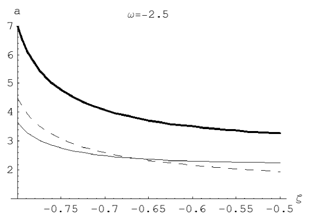
Figure 1: The region below the thick line satisfies $\sigma+p\geq 0$ and the region below the thin line satisfies $\sigma\geq 0$. The dashed line corresponds to Eq. (59).

4 Stable solutions

In section 3, we have found all the solutions satisfying the WEC. Our task in this section is to check whether these solutions can be stable, i.e., whether $V^{\prime\prime}(a)<0$ can be satisfied. Note that from Eq. (51) the value of $V^{\prime\prime}(a)$ also depends on the parameter $\beta^{2}$. By substituting Eq. (59) into Eq. (51), one can express $V^{\prime\prime}(a)$ as a function of $\zeta$

$$V^{\prime\prime}(\zeta)=\tilde{V}(\zeta)g(\zeta)\,,$$ (69)

where $g(\zeta)$ is positive in the allowed range of $\zeta$ and

$$\tilde{V}(\zeta) = (-2\omega^{2}-2\beta^{2}\omega^{2}-\omega^{3}-2\beta^{2}\omega^{3})\zeta^{2}+(2\omega+8\beta^{2}\omega+8\beta^{2}\omega^{2})\zeta$$ (70)

$$+ (-6-\beta^{2}-3\omega-6\beta^{2}\omega)\,.$$

The stability condition $V^{\prime\prime}(\zeta)<0$ is equivalent to $\tilde{V}(\zeta)<0$ , i.e.,

$$2(1+\omega)(3-4\omega\zeta+\omega^{2}\zeta^{2})\beta^{2}>-6-3\omega+2\omega\zeta-2\omega^{2}\zeta^{2}-\omega^{3}\zeta^{2}$$ (71)

One can show

$$(1+\omega)(3-4\omega\zeta+\omega^{2}\zeta^{2})>0\,.$$ (72)

Eq. (71) is equivalent to

$$\beta^{2}>f_{\beta}(\zeta)\equiv\frac{-6-3\omega+2\omega\zeta-2\omega^{2}\zeta^{2}-\omega^{3}\zeta^{2}}{2(1+\omega)(3-4\omega\zeta+\omega^{2}\zeta^{2})}\,.$$ (73)

Our goal is to find the minimum $f_{\beta}(\zeta)$ within the range $\zeta_{1}<\zeta<\zeta_{2}$ for each $\omega<-2$. We first consider

$$f_{\beta}^{\prime}(\zeta)=\frac{\omega(3+2\omega)(-3+\omega^{2}\zeta^{2})}{(1+\omega)(3-4\omega\zeta+\omega^{2}\zeta^{2})^{2}}\,.$$ (74)

The condition

$$f_{\beta}^{\prime}(\zeta)>0$$ (75)

is equivalent to

$$-3+\omega^{2}\zeta^{2}<0\,,$$ (76)

i.e.,

$$\zeta>\frac{\sqrt{3}}{\omega}\,.$$ (77)

By solving

$$\frac{\sqrt{3}}{\omega}<\zeta_{1}\,.$$ (78)

we have

$$\omega<\frac{\sqrt{3}}{1-\sqrt{3}}\approx-2.366\,.$$ (79)

In this range, Eq. (77) and then Eq. (75) always hold. Consequently, for given $\omega$, the minimum required $\beta^{2}$ is given by

$$\beta_{min}^{2}(\omega)=f_{\beta}(\zeta=\zeta_{1})=\frac{2+3\omega+2\omega^{2}}{-2-2\omega}\,,$$ (80)

where $\zeta_{1}=\frac{1}{1+\omega}$.

For

$$-2.366<\omega<-2\,,$$ (81)

$f_{\beta}(\zeta)$ decreases in the range $\zeta_{1}<\zeta<\frac{\sqrt{3}}{\omega}$ and increases in the range $\frac{\sqrt{3}}{\omega}<\zeta<\zeta_{2}$. Hence, The minimum value of $f_{\beta}(\zeta)$ is attained at $\zeta=\frac{\sqrt{3}}{\omega}$. By substitution, we have the minimum as a function of $\omega$

$$\beta^{2}_{min}(\omega)=\frac{6-\sqrt{3}+3\omega)}{2(-3+2\sqrt{3})(1+\omega)}\,.$$ (82)

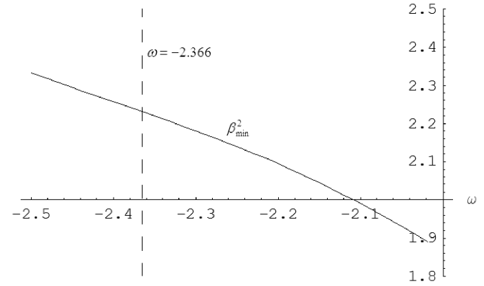
Figure 2: Plot of $\beta_{min}^{2}$ as a function of $\omega$. $\beta^{2}_{min}$ achieve a minimum at $\omega=-2$.

Combing Eqs. (80) and (82), one has the function $\beta_{min}^{2}(\omega)$ defined in $-\infty<\omega<-2$. As depicted in Fig. 2, we see $\beta_{min}^{2}$ changes smoothly across $\omega=-2.366$. Obviously, $\beta^{2}_{min}$ decreases monotonically with $\omega$ and attains its minimum value

$$\beta^{2}_{0}=\frac{\sqrt{3}}{2(-3+2\sqrt{3})}\approx 1.866$$ (83)

at $\omega=-2$. Hence no stable solutions exist for $\beta^{2}<\beta_{0}^{2}$.

5 Conclusions

We have reexamined the Brans-Dicke thin-shell wormhole model discussed in [9] and found all stable solutions satisfying the WEC. The constraint equations listed in [9] have been solved analytically. These solutions require $\omega<-2$. We have also found the exact parameter range of $\zeta$. For each $\omega$, the stability condition requires a minimum $\beta^{2}$ that decreases monotonically with $\omega$. Hence the minimum $\beta^{2}$ required for a stable solution is $\beta_{0}^{2}=1.866$, which is attained at $\omega=-2$.

Our work shows that Brans-Dicke thin-shell wormholes can be supported by matter without violating the WEC and be stable against linear perturbation. To the best of our knowledge, this is the first example in four-dimensional spacetimes confirming the existence of stable wormholes that do not violate the WEC. However, our calculation rules out any stable solutions for $\beta^{2}\leq 1$. This means the speed of sound at the throat of the wormhole must exceed the speed of light. Usually, such a solution is not acceptable because causality may be violated. However, whether superluminal behavior causes violation of causality has become a subtle and controversial issue in recent years (see e.g. [13]-[15]). We think the problem is still open and the configurations with $\beta^{2}>1$ should not be ruled out.

Appendix A Calculation for $\omega>-3/2$

We shall show that no solutions exist in the range $\omega>-3/2$. Let us first consider the constraint $a>2$. It follows immediately from Eq. (62) that

$$f(\zeta)>2\,.$$ (84)

The roots of $f(\zeta)=2$ are

$$\zeta=\frac{-\omega\pm\sqrt{2}\sqrt{3\omega+2\omega^{2}}}{2\omega+\omega^{2}}\,.$$ (85)

For $-3/2<\omega\leq 0$, the roots do not exist. Note that $f^{\prime}(\zeta)$ increases monotonically in this range. Thus, Eq. (84) cannot be fulfilled. So the range of $\omega$ is restricted to $\omega>0$. In this case, Eq. (84) requires

$$\zeta>\frac{-\omega+\sqrt{2}\sqrt{3\omega+2\omega^{2}}}{2\omega+\omega^{2}}>0\,.$$ (86)

Using Eq. (64) , the constraint (LABEL:fs) is equivalent to

$$\zeta<\frac{1}{1+\omega}\,.$$ (87)

However, it is not hard to show that

$$\frac{-\omega+\sqrt{2}\sqrt{3\omega+2\omega^{2}}}{2\omega+\omega^{2}}>\frac{1}{1+\omega}\,.$$ (88)

for any $\omega>0$. Therefore, no solutions satisfying the constraints can be found for $\omega>-3/2$.

References

[1] M.S.Morris and K.S. Thorne, Am.J.Phys. 56,395(1988).
[2]M. Visser, Phys. Rev. D 39, 3182 (1989).
[3] W. Israel, Nuovo Cimento 44 B, 1 (1966); ibid.48B, 463,Erratum(1967).
[4]E.Poisson, M. Visser, Phys. Rev. D 52, 7318 (1995).
[5] M. Richarte, C. Simeone, Phys.Rev. D 76, 087502.
(2007)
[6] J.P.S.Lemos and F.S.N. Lobo,Phys.Rev.D 78 044030 (2008).
[7]M. Visser, Phys. Rev. Lett. 90, 201102 (2003).
[8] S.H.Mazharimousavi, M. Halilsoy and Z.Amirabi, Phys. Rev. D 81, 104002 (2010).
[9] Ernesto F. Eiroa, Martin G. Richarte, Claudio
Simeone, Phys.Lett. A373 (2008) 1-4;Erratum-ibid. A373 (2009)
2399-2400.
[10] F.S. N. Lobo and P. Crawford, Class.Quant.Grav. 22, 4869 (2005).
[11] E. Eiroa and G. Romero, Gen. Rel. Grav. 36,
651 (2004).
[12] A.G. Agnese and M. La Camera, Phys. Rev. D 51, 2011 (1995).
[13] G.Ellis, R. Maartens, M. MacCallum, Gen.Rel.Grav. 391651 (2007).
[14] J.P.Bruneton, Phys. Rev. D 75, 085013 (2007).
[15] E. Babichev, V.F.Mukhanov and A.Vikman, JHEP 0609 (2006) 061.