Numerical study of the derivative of the Riemann zeta function at zeros

Abstract.

The derivative of the Riemann zeta function was computed numerically on several large sets of zeros at large heights. Comparisons to known and conjectured asymptotics are presented.

Dedicated to Professor Akio Fujii on his retirement.

1. Introduction

Throughout this paper, we assume the truth of the Riemann Hypothesis (RH), and we let $\gamma_{n}>0$ denote the ordinate of the $n$-th non-trivial zero of $\zeta(s)$. Hejhal [He] assumed the RH and a weak consequence of Montgomery’s [Mo] pair-correlation conjecture, namely that for some $\tau>0$, there is a constant $B$ such that

(1.1) $$\limsup_{N\to\infty}\frac{1}{N}\left|\{n\,:\,N\leq n\leq 2N\,,\,(\gamma_{n+1}-\gamma_{n})\log\gamma_{n}<c\}\right|\leq Bc^{\tau}\,,$$

holds for all $c\in(0,1)$. Under these assumptions, he proved the following central limit theorem: for $\alpha<\beta$,

(1.2) $$\lim_{N\to\infty}\frac{1}{N}\,\left|\left\{n\,:\,N\leq n\leq 2N\,,\,\frac{\log\left|\displaystyle\frac{2\pi\zeta^{\prime}(1/2+i\gamma_{n})}{\log(\gamma_{n}/2\pi)}\right|}{\sqrt{\frac{1}{2}\log\log N}}\in(\alpha,\beta)\right\}\right|=\frac{1}{\sqrt{2\pi}}\int_{\alpha}^{\beta}e^{-x^{2}/2}\,dx\,,$$

So under these assumptions, $\log|\zeta^{\prime}(1/2+i\gamma_{n})|$, suitably normalized, converges in distribution over fixed ranges to a standard normal variable. To obtain more precise information about the tails of the distribution, we consider the moments

(1.3) $$J_{\lambda}(T):=\frac{1}{N(T)}\sum_{0<\gamma_{n}\leq T}|\zeta^{\prime}(1/2+i\gamma_{n})|^{2\lambda}\,,$$

where $N(T):=\sum_{0<\gamma_{n}\leq T}1=\frac{T}{2\pi}\log\frac{T}{2\pi e}+O(\log T)$ is the zero counting function. Notice that $J_{\lambda}(T)$ is defined for all $\lambda$ provided the zeros of $\zeta(s)$ are simple, as is widely believed.

Gonek [Go1] [Go2] carried out an extensive study of $J_{\lambda}(T)$. He proved, under the assumption of the RH, that $J_{1}(T)\sim\frac{1}{12}(\log T)^{3}$ as $T\to\infty$. It was suggested by Gonek [Go2], and independently by Hejhal [He], that $J_{\lambda}(T)$ is on the order of $(\log T)^{\lambda(\lambda+2)}$. Ng [Ng] proved, under the RH, that $J_{2}(T)$ is order of $(\log T)^{8}$, which is in agreement with that suggestion.

Hughes, Keating, and O’Connell [HKO], applied the random matrix philosophy (e.g. see [KS]), which predicts that certain behaviors of $L$-functions are mimicked statistically by characteristic polynomials of large matrices from the classical compact groups. This led them to predict that for Re($\lambda$) $>-3/2$,

(1.4) $$J_{\lambda}(T)\sim a(k)\frac{G^{2}(\lambda+2)}{G(2\lambda+3)}\left(\log\frac{T}{2\pi}\right)^{\lambda(\lambda+2)}~{}~{}~{}~{}~{}~{}{\hbox{as}}~{}~{}~{}~{}~{}~{}~{}~{}~{}~{}T\to\infty,$$

where $G(z)$ is the Barnes G-function, and $a(k)$ is an “arithmetic factor.” The conjecture (1.4) is consistent with previous theorems and conjectures.

Recently, Conrey and Snaith [CS], assuming the ratios conjecture, gave lower order terms in asymptotic expansions for $J_{1}(T)$ and $J_{2}(T)$. They conjectured the existence of certain polynomials $P_{\lambda}(x)$, for $2\lambda=2$ and $2\lambda=4$, such that

(1.5) $$\sum_{0<\gamma_{n}<T}|\zeta^{\prime}(1/2+i\gamma_{n})|^{2\lambda}\sim\int_{0}^{T}P_{\lambda}\left(\log\frac{t}{2\pi}\right)\,dt\,,$$

The conjecture for the case $2\lambda=2$ was subsequently proved by Milinovich [Mi], assuming the RH. It is expected that such polynomials exist for other integer values of $\lambda>0$ as well.

The purpose of this article is to study numerically various statistics of the derivative of the zeta function at its zeros. In particular, we consider the distribution of $\log|\zeta^{\prime}(1/2+i\gamma_{n})|$, moments of $|\zeta^{\prime}(1/2+i\gamma_{n})|$, and correlations among moments. The goal is to obtain more detailed information about the derivative at zeros, and to enable comparison with various conjectured and known asymptotics. Our computations rely on large sets of zeros at large heights that are described in detail in [HO].

We find that the empirical distribution of $\log|\zeta^{\prime}(1/2+i\gamma_{n})|$, normalized to have mean zero and standard deviation one, agrees generally well with the limiting normal distribution proved by Hejhal, as shown in Figure 1. But the empirical mean and standard deviation pre-normalization are noticeably different from predicted ones. Also, as shown in Figure 2, the frequency of very small normalized values of $\log|\zeta^{\prime}(1/2+i\gamma_{n})|$ is higher than predicted by a standard normal distribution, while the frequency of very large normalized values is lower than predicted. Since these differences appear to decrease steadily with height, however, they are probably not significant.

To examine the tails of the distribution of $\log|\zeta^{\prime}(1/2+i\gamma_{n})|$, we present data for the moments of $|\zeta^{\prime}(1/2+i\gamma_{n})|$ over short ranges:

(1.6) $$J_{\lambda}(T,H):=\frac{1}{N(T+H)-N(T)}\sum_{T\leq\gamma_{n}\leq T+H}|\zeta^{\prime}(1/2+i\gamma_{n})|^{2\lambda}.$$

For large $\lambda$, the empirical values of $J_{\lambda}(T,H)$ deviate substantially from the values suggested by the leading term prediction (1.4). This is not surprising. Because for $\lambda$ large relative to $T$, the contribution of lower order terms is likely to dominate, and so the leading term asymptotic on its own may not suffice. Furthermore, the said deviations decrease steadily with height and they occur in a generally uniform way for roughly $2\lambda\leq 6$, so they are consistent with the effect of “lower order terms” still being felt even at such relatively large heights.

In the specific cases of the second and fourth moments of $|\zeta^{\prime}(1/2+i\gamma_{n})|$, the conjectures of Conrey and Snaith [CS] supply lower order terms, and the agreement with the data is much better, as shown in Table 4.

As $\lambda$ increases, the observed variability in the moments of $|\zeta^{\prime}(1/2+i\gamma_{n})|$ is more extreme, but it is still significantly less than we previously encountered in the moments of $|\zeta(1/2+it)|$ (see [HO]). To illustrate, our computations of the twelfth moment of $|\zeta^{\prime}(1/2+i\gamma_{n})|$ over 15 separate sets of $\approx 10^{9}$ zeros each (near the $10^{23}$-rd zero) show that the ratio of highest to lowest moment among the 15 twelfth moments thus obtained was 2.36. In contrast, that ratio for the twelfth moment of $|\zeta(1/2+it)|$ was 16.34, which is significantly larger (see [HO]).

In general, the variability in statistical data for $|\zeta^{\prime}(1/2+i\gamma_{n})|$ is considerably less than the variability in statistical data for $|\zeta(1/2+it)|$. It is not immediately clear why this should be so, considering, for instance, that the central limit theorem for $\log|\zeta^{\prime}(1/2+i\gamma_{n})|$ is only conditional, while that for $\log|\zeta(1/2+it)|$ is not, and both theorems scale by the same asymptotic variance.

In the case of negative moments, our data is in agreement with Gonek’s conjecture ([Go1]) $J_{-1}(T)\sim\frac{6}{\pi^{2}}(\log T/(2\pi))^{-1}$ as $T\to\infty$. But starting at $2\lambda=-3$, and as $\lambda$ decreases, the empirical behavior of negative moments becomes rapidly more erratic. For example, using the same 15 zero sets near the $10^{23}$-rd zero mentioned previously, the ratio of highest to lowest negative moment among them gets very large as $\lambda$ decreases; we obtain: 1.03, 8.45, 178.49, and 17240.99, for $2\lambda=-2,-3,-4,$ and $-6$, respectively (this can be deduced easily from Table 6). Notice that the point $2\lambda=-3$ is special because it is where the leading term prediction (1.4) first breaks down due to a pole of order 1 in the ratio of Barnes G-functions.

Extreme values of negative moments are caused by very few zeros. When $2\lambda=-3$, for instance, the largest observed moment among our 15 sets is $0.178047$. About 87% of this value is contributed by 4 zeros where $|\zeta^{\prime}(1/2+i\gamma_{n})|$ is small and equal to 0.002439, 0.002453, 0.004388, and 0.004365. Such small values of $|\zeta^{\prime}(1/2+i\gamma)|$ typically occur at pairs of consecutive zeros that are close to each other. For example, the values 0.002439 and 0.002453 occur at the following two consecutive zero ordinates:

(1.7) $$\begin{split}&1.30664344087942265202071895041619\times 10^{22}\,,\\ &1.30664344087942265202071898265199\times 10^{22}\,.\end{split}$$

The above pair of zeros is separated by 0.00032, which is about 1/400 times the average spacing of zeros at that height (which is $\approx 0.128$).

To investigate possible correlations among values of $|\zeta^{\prime}(1/2+i\gamma_{n})|^{2\lambda}$, we studied numerically the (shifted moment) function:

(1.8) $$S_{\lambda}(T,H,m):=\sum_{T\leq\gamma_{n}\leq T+H}|\zeta^{\prime}(1/2+i\gamma_{n})\zeta^{\prime}(1/2+i\gamma_{n+m})|^{2\lambda}\,.$$

We plotted $S_{\lambda}(T,H,m)$, for several choices of $\lambda$, $T$, and $H$, and as $m$ varies. The resulting plots indicate there are long-range correlations among the values of the derivative at zeros. Unexpectedly, the tail of $S_{2}(T,H,m)$ (Figure 3; right plot) strongly resembles the tail for the shifted fourth moment of $|\zeta(1/2+it)|$ (Figure 4 in [HO]).

To better understand these correlations, we considered the “spectrum” of $\log|\zeta^{\prime}(1/2+i\gamma_{n})|$; see (2.6) for a definition. A plot of the spectrum reveals sharp spikes, shown in Figure 5. These spikes can be explained heuristically by applying techniques already used by Fujii [Fu, Fu2] and Gonek [Go1] to estimate sums involving $\zeta^{\prime}(1/2+i\gamma_{n})$.

2. Numerical results

Conjecture (1.2) suggests the mean and standard deviation of $\log|\zeta^{\prime}(1/2+i\gamma)|$ for zeros from near $T=1.3066434\times 10^{22}$ (i.e. near the $10^{23}$-rd zero) are about 2.0 and 1.4, respectively. This is far from the empirical mean and standard deviations listed in Table 1, which are 3.4907 and 1.0977. Since these quantities grow very slowly (like $\log\log T$), these differences are probably not significant.

Table 1. Summary statistics for $\log|\zeta^{\prime}(1/2+i\gamma_{n})|$ using sets of $10^{7}$ zeros from different heights The column ”Zero” lists the zero number near which the set is located. SD stands for standard deviation.

Zero	Min	Max	Mean	SD
$10^{16}$	-3.7371	7.3920	3.1211	1.0135
$10^{20}$	-3.2181	8.0085	3.3458	1.0653
$10^{23}$	-2.9602	8.2836	3.4907	1.0977

We normalize the sequence $\{\log|\zeta^{\prime}(1/2+i\gamma_{n})|\,:\,N\leq n\leq N+10^{7}\}$, where $N\approx 10^{23}$, to have mean zero and variance one. The distribution of the normalized sequence is illustrated in Figure 1, which contains two plots, one of the empirical density function, and another of the difference between the empirical density and the predicted (standard Gaussian) density $\frac{1}{\sqrt{2\pi}}e^{-x^{2}/2}$. The fit in the first plot is visibly good, but there is a slight shift to the right about the center. This shift is made more visible in the second plot, which shows that the empirical density is generally larger than expected for $x>0$, and is smaller than expected for $x<0$.

Figure 1. Empirical density of $\log|\zeta^{\prime}(1/2+i\gamma_{n})|$, after being normalized to have mean 0 and standard deviation 1, using $10^{7}$ values of $\log|\zeta^{\prime}(1/2+i\gamma_{n})|$ from near the $10^{23}$-rd zero (the bin size is $0.0512$). The density of a standard normal variable (continuous line) is drawn to facilitate comparison. The right plot shows the diference, the empirical density minus the normal.

Near the tails, however, the situation is reversed. Figure 2 shows there is a deficiency in the occurrence of very large values of $|\zeta^{\prime}(1/2+i\gamma_{n})|$, and an abundance in the occurrence of very small values. For instance, conjecture (1.2) suggests that about 0.1462% of the values of $|\zeta^{\prime}(1/2+i\gamma_{n})|$ near the $10^{23}$-rd zero should satisfy $|\zeta^{\prime}(1/2+i\gamma_{n})|>860$, which is noticeably larger than the observed 0.1056%. The conjecture also suggests about 0.0736% of the values should satisfy $|\zeta^{\prime}(1/2+i\gamma_{n})|<1$, which is smaller than the observed 0.1051%.

We remark the behavior near the tails becomes more consistent with expectation as height increase . For example, only 0.0025% of the time do we have $\log|\zeta^{\prime}(1/2+i\gamma_{n})|>3.2$ near the $10^{16}$-th zero, which is far from the expected 0.068%, but the percentage increases to 0.040% near the $10^{23}$-rd zero.

Figure 2. Distribution at the tails using $1.5\times 10^{10}$ zeros near the $10^{23}$-rd zero (bin size is 0.01).

For another measure of the quality of the fit to the standard Gaussian in Figure 1, we compare moments of both distributions. Table 2 shows the first few moments (the even moments in particular) agree reasonably well. Notice the odd moments tend to be negative, which is likely due to the aforementioned bias in the frequency of very small and very large values.

Table 2. Moments of $\log|\zeta^{\prime}(1/2+i\gamma_{n})|$, after being normalized to have mean zero and variance one, calculated using $10^{7}$ zeros from near the $10^{23}$-rd zero. The third column is the moment of a standard Gaussian.

Moment	Derivatives	Gaussian
3rd	-0.02728	0
4th	3.01364	3
5th	-0.49120	0
6th	15.3053	15
7th	-7.43073	0
8th	112.013	105
9th	-118.588	0
10th	1116.64	945

To better understand the tails of the distribution of $\log|\zeta^{\prime}(1/2+i\gamma_{n})|$, we consider the moments $J_{\lambda}(T)$ defined in (1.3). Since we are interested in the asymptotic behavior of $J_{\lambda}(T)$, we compare against the leading term prediction (1.4). We calculated ratios of the form

(2.1) $$\frac{\frac{1}{|B|}\sum_{\gamma\in B}|\zeta^{\prime}(1/2+i\gamma)|^{2\lambda}}{a(\lambda)\frac{G^{2}(\lambda+2)}{G(2\lambda+3)}\left(\log\frac{T}{2\pi}\right)^{\lambda(\lambda+2)}}\,,$$

where $B$ is a block of consecutive zeros, $|B|$ denotes the number of zeros in $B$, and $T$ is the height where block $B$ lies. If $T$ is large enough, one expects the value of (2.1) to approach 1 as the block size $|B|$ increases. Table 3, which uses blocks of size $|B|\approx 10^{9}$ (except for the first set, which uses the first $10^{8}$ zeta zeros), shows that the empirical moments are significantly larger than the corresponding predictions, even for low moments. For example, the empirical second moments ($2\lambda=2$) near the $10^{23}$-rd zero are generally off from expectation by about 9.6%.

Nevertheless, the ratios (2.1) appear to decrease towards the expected 1 as the height increases, and there is relatively little variation in the moment data for sets from near the same height when $2\lambda\leq 6$. Both of these observations are consistent with the “lower order terms” still contributing significantly.

Table 3. Ratio (2.1) calculated with $|B|\approx 10^{9}$, except for the first set, which uses the first $10^{8}$ zeros. The column “Zero” lists the approximate zero number near which block $B$ is located.

Zero	$2\lambda=2$	$2\lambda=4$	$2\lambda=6$	$2\lambda=8$	$2\lambda=10$	$2\lambda=12$
$10^{8}$	1.1247	3.1579	91.856	78341	$4.1016\times 10^{9}$	$2.3478\times 10^{16}$
$10^{16}$	1.1424	2.2087	17.686	1266.9	$1.5057\times 10^{6}$	$4.9628\times 10^{10}$
$10^{20}$	1.1123	1.9102	10.943	422.72	$1.9904\times 10^{5}$	$1.8362\times 10^{9}$
$10^{23}$	1.0964	1.7645	8.4406	233.63	$6.4583\times 10^{4}$	$2.7127\times 10^{8}$
-	1.0964	1.7603	8.1602	199.18	$4.1647\times 10^{4}$	$1.1369\times 10^{8}$
-	1.0964	1.7598	8.1879	202.40	$4.3355\times 10^{4}$	$1.2325\times 10^{8}$
-	1.0964	1.7629	8.3221	217.58	$5.2539\times 10^{4}$	$1.7809\times 10^{8}$
-	1.0964	1.7630	8.3861	228.51	$6.2549\times 10^{4}$	$2.6614\times 10^{8}$
-	1.0964	1.7600	8.2022	206.36	$4.6423\times 10^{4}$	$1.4200\times 10^{8}$
-	1.0965	1.7642	8.3321	218.38	$5.3663\times 10^{4}$	$1.8923\times 10^{8}$
-	1.0965	1.7612	8.1862	201.43	$4.3256\times 10^{4}$	$1.2547\times 10^{8}$
-	1.0963	1.7590	8.2176	209.97	$4.8853\times 10^{4}$	$1.5596\times 10^{8}$
-	1.0964	1.7654	8.3856	217.09	$4.8781\times 10^{4}$	$1.4148\times 10^{8}$
-	1.0963	1.7616	8.3009	218.92	$5.4691\times 10^{4}$	$1.9491\times 10^{8}$
-	1.0964	1.7585	8.1576	204.55	$4.6872\times 10^{4}$	$1.5134\times 10^{8}$
-	1.0965	1.7615	8.2380	209.26	$4.7946\times 10^{4}$	$1.5078\times 10^{8}$
-	1.0963	1.7586	8.1764	203.00	$4.4241\times 10^{4}$	$1.2904\times 10^{8}$
-	1.0964	1.7603	8.2037	208.39	$4.9019\times 10^{4}$	$1.6822\times 10^{8}$

The full moment prediction of [CS], which takes lower order terms into account, might lead one to expect that for $2\lambda=2$, $2\lambda=4$, as $T\to\infty$, and for blocks $B$ not too small compared to $T$,

(2.2) $$\sum_{\gamma\in B}|\zeta^{\prime}(1/2+i\gamma)|^{2\lambda}\sim\int_{B}P_{\lambda}(\log(t/2\pi))\,dt\,,$$

where $P_{\lambda}(x)$ is as given in [CS], and $\int_{B}$ is short for integrating over the interval spanned by the block $B$. To test this, we calculated ratios of the form

(2.3) $$\frac{\sum_{\gamma\in B}|\zeta^{\prime}(1/2+i\gamma)|^{2\lambda}}{\int_{B}P_{\lambda}(\log(t/2\pi))\,dt}\,.$$

As the block size increases, we expect (2.3) to be significantly closer to 1 than (2.1) since it relies on a more accurate prediction. This is indeed what Table 4 illustrates, where we see the fit to moment data is much better than we found in Table 3. (We point out that in the case $2\lambda=4$ only the first three terms in the full moment conjecture were used, because these were the only terms provided explicitly in [CS]. It is likely the fit to the data will be even better if the missing terms are included.)

Table 4. Ratio (2.3) calculated with $|B|\approx 10^{9}$, except for the first set, which uses the first $10^{8}$ zeros. The column “Zero” lists the approximate zero number near which block $B$ is located.

Zero	$2\lambda=2$	$2\lambda=4$
$10^{8}$	1.0000	1.0924
$10^{16}$	1.0000	1.0144
$10^{20}$	1.0000	1.0087
$10^{23}$	1.0000	1.0074
“	1.0000	1.0050
“	0.9999	1.0047
“	1.0000	1.0064
“	0.9999	1.0065
“	0.9999	1.0048
“	1.0000	1.0072
“	1.0000	1.0055
“	0.9998	1.0042
“	1.0000	1.0079
“	0.9999	1.0057
“	0.9999	1.0039
“	1.0000	1.0057
“	0.9999	1.0040
“	1.0000	1.0049

We remark that the five largest values of $|\zeta^{\prime}(1/2+i\gamma_{n})|$ in our data set are $\approx$ 7057, 6907, 6658, 6636, and 6399. The cumulative contribution of these large values to the $2\lambda$-th moment, as a percentage of the overall $2\lambda$-th moment, is listed in Table 5 for several $\lambda$.

Table 5. Cumulative contribution percentage of the 5 largest values of $|\zeta^{\prime}(1/2+i\gamma_{n})|$ to the empirical $2\lambda$-th moment for $1.5\times 10^{10}$ zeros near the $10^{23}$-rd zero.

$2\lambda=8$	$2\lambda=10$	$2\lambda=12$
0.50	1.84	4.51
0.92	3.32	7.99
1.24	4.35	10.2
1.54	5.35	12.3
1.77	6.04	13.7

In the case of negative moments, the conjecture $J_{-1}(T)\sim\frac{6}{\pi^{2}}(\log T/(2\pi))^{-1}$ as $T\to\infty$, due to Gonek [Go2], suggests the negative second moment should be $\approx 0.01808$ near zero number $10^{16}$, $\approx 0.01436$ near zero number $10^{20}$, and $\approx 0.01238$ near zero number $10^{23}$. These predictions are in good agreement with the values listed in Table 6.

For $2\lambda\leq-3$, the behavior is much less predictable because, empirically, their sizes are determined by a few zeros where $|\zeta^{\prime}(1/2+i\gamma_{n})|$ is small. In fact, the particularly large fluctuations in the size of the negative sixth moment ($2\lambda=-6$), near the $10^{23}$-rd zero in Table 6, are essentially due to 8 zeros (out of $1.5\times 10^{10}$) where $|\zeta^{\prime}(1/2+i\gamma_{n})|$ is equal to 0.002439, 0.002453, 0.002719, 0.002737, 0.003094, 0.003108, 0.004365, and 0.004388.

Table 6. Ratio (2.3) calculated with $|B|\approx 10^{9}$, except for the first set, which uses the first $10^{8}$ zeros. The column “Zero” lists the approximate zero number near which block $B$ is located.

Zero	$2\lambda=-2$	$2\lambda=-3$	$2\lambda=-4$	$2\lambda=-6$
$10^{8}$	0.041129	0.059025	1.04212	2935.6
$10^{16}$	0.018057	0.030660	0.55588	1488.1
$10^{20}$	0.014341	0.028403	0.73586	2873.2
$10^{23}$	0.012347	0.022040	0.41441	1106.5
“	0.012365	0.022605	0.43869	1314.6
“	0.012462	0.037677	2.76255	63336
“	0.012321	0.021618	0.42275	1431.0
“	0.012776	0.178047	59.6610	9288238
“	0.012326	0.021062	0.33853	665.29
“	0.012515	0.052929	7.46570	412318
“	0.012334	0.022429	0.56305	4157.4
“	0.012376	0.025800	0.81652	5414.6
“	0.012541	0.089163	21.5695	2174342
“	0.012411	0.039415	4.32860	185114
“	0.012329	0.022729	0.55154	2723.6
“	0.012386	0.027487	1.08706	11563
“	0.012605	0.117993	35.4067	4686740
“	0.012334	0.021217	0.33424	538.73

Starting with the investigations of [Od2], several long-range correlations have been found experimentally in zeta function statistics. Such correlations are not present in random matrices, but do appear in some dynamical systems that for certain ranges are modeled by random matrices. So far all the zeta function correlations of this nature have been explained (at least numerically and heuristically) by relating them to known properties of the zeta function, such as explicit formulas that relate primes to zeros. A natural question is whether such correlations arise among values of $\zeta^{\prime}(1/2+i\gamma_{n})$.

In order to detect correlations among values of $|\zeta^{\prime}(1/2+i\gamma_{n})|$, consider

(2.4) $$S_{2}(T,H,m):=\sum_{T\leq\gamma_{n}\leq T+H}|\zeta^{\prime}(1/2+i\gamma_{n})\zeta^{\prime}(1/2+i\gamma_{n+m})|^{4}\,.$$

We computed this shifted moment function for various choices of $m$, $T$, and $H$. (We also considered similar sums with exponents other than 4, but for simplicity do not discuss them here.) Figure 3 presents some of our results near the $10^{16}$-th and $10^{23}$-rd zeros, and with $H$ spanning about $10^{7}$ zeros in both cases. The figure shows that correlations do exist and persist over long ranges. Also, the shape of $S_{2}(T,H,m)$ near the $10^{16}$-th zero is similar to that near the $10^{23}$-rd zero, except the former has higher peaks, and covers the range $3\leq m\leq 222$, as opposed to $3\leq m\leq 325$, which suggests oscillations scale as $1/\log(T/2\pi)$.

We remark the plot of $S_{2}(T,H,m)$ in Figure 3 (right plot) is similar to a plot in [HO] of the shifted fourth moment of the zeta function on the critical line:

(2.5) $$M(T,H;\alpha):=\int_{T}^{T+H}|\zeta(1/2+it)|^{2}\,|\zeta(1/2+it+i\alpha)|^{2}\,dt\,,$$

which we reproduce here in Figure 4 for the convenience of the reader.

Figure 3. Plots of $S_{2}(T,H,m)/S_{2}(T,H,0)$ using $10^{7}$ zeros near the $10^{16}$-th (left plot) and the $10^{23}$-rd zero (right plot)

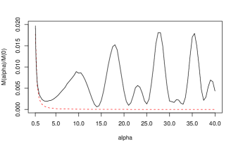
Figure 4. Plot of $M(T,H,\alpha)/M(T,H,0)$, with $H\approx 6.5\times 10^{5}$, near the $10^{23}$-rd zero, drawn for $\alpha$ a multiple of $0.5$. The dashed line is a sine kernel.

To explain observed correlations, we numerically calculated the function:

(2.6) $$f(T,H,x)=\left|\sum_{T\leq\gamma_{n}\leq T+H}\zeta^{\prime}(1/2+i\gamma_{n})e^{2\pi inx}\right|\,,$$

which is related to long-range periodicities in $\zeta^{\prime}(1/2+i\gamma_{n})$. Assuming the RH, Fujii [Fu] supplied the following asymptotic formula in the case $x=0$:

(2.7) $$\sum_{0<\gamma_{n}\leq T}\zeta^{\prime}(1/2+i\gamma_{n})=\frac{T}{4\pi}\log^{2}\frac{T}{2\pi}+(c_{0}-1)\frac{T}{2\pi}\log\frac{T}{2\pi}-(c_{1}+c_{0})\frac{T}{2\pi}+O\left(T^{1/2}\log^{7/2}T\right)\,,$$

where $c_{0}=0.5772\ldots$ (the Euler constant) and $c_{1}=-0.0728\ldots$. Empirical values of $f(T,H,0)$ agree well with formula (2.7). For example, with $H$ spanning $10^{6}$ zeros, we obtain $f(T,H,0)=21766088-14579i$ near the $10^{20}$-zero, and we obtain $f(T,H,0)=25137126+61663i$ near the $10^{23}$-rd zero. But as $x$ increases, $f(T,H,x)$ experiences sharp spikes for certain $x$, as shown in Figure 5, which depicts the segment $0\leq x\leq 0.05$ (in the remaining portion $0.05<x<1$, the spikes get progressively denser).

The sharp spikes in Figure 5 show the existence of long-range periodicities among values of $\zeta^{\prime}(1/2+i\gamma_{n})$. These spikes, as well as the correlations described above, are not unexpected. They can be demonstrated to follow from the properties of the zeta function, by estimating proper contour integrals. Such methods were used for continuous averages by Ingham [Ingh] and even others before him, and for discrete averages over zeros by Gonek [Go1] and Fujii [Fu, Fu2]. The main step involves integration of ${\zeta^{\prime}(s)}^{2}/{\zeta(s)}$, and estimates of such integrals.

Applying such methods to ${\zeta^{\prime}(s)}^{2}e^{xs\log\frac{T}{2\pi}}/{\zeta(s)}$ suggests that the function

$$\tilde{f}(T,H,x)=\left|\sum_{T\leq\gamma_{n}\leq T+H}\zeta^{\prime}(1/2+i\gamma_{n})e^{2\pi i\tilde{\gamma}_{n}x}\right|\,,\qquad\tilde{\gamma}_{n}:=\frac{\gamma_{n}}{2\pi}\,\log\frac{T}{2\pi}\,,$$

experiences large spikes at approximately $x=\log(k)/\log(T/(2\pi))$. For by a heuristic argument involving the (very) regular spacing of zeros one expects that $\tilde{\gamma}_{n}$ in the definition of $\tilde{f}(T,H,x)$ can be replaced by $n$ without too much error (see [Od2] for a similar argument in the context of long-range correlations in zero spacings). Therefore, $f(T,H,x)$ should behave similarly to $\tilde{f}(T,H,x)$. In particular, we expect the $k$-th spike in Figure 5 to occur at approximately $\log(k)/\log(T/(2\pi))$, and that agrees well with the evidence of the graphs.

Figure 5. Plots of $f(T,H,x)$, defined in (2.6), using $10^{6}$ zeros near the $10^{16}$-th zero (upper left), $10^{20}$-rd zero (upper right), and $10^{23}$-rd zero (lower left). The lower right plot is another plot near the $10^{23}$-rd zero, except it uses a different set of $2\times 10^{6}$ zeros.

3. Numerical methods

As usual, define the rotated zeta function on the critical line by

(3.1) $$Z(t)=e^{i\theta}\zeta(1/2+it)\,,\qquad e^{i\theta(t)}=\left(\frac{\Gamma(1/4+it/2)}{\Gamma(1/4-it/2)}\right)^{1/2}\pi^{-it/2}\,.$$

The rotation factor $e^{i\theta(t)}$ is chosen so that $Z(t)$ is real. In our numerical experiments, $t<1.31\times 10^{22}$.

Since $|Z^{\prime}(\gamma_{n})|=|\zeta^{\prime}(1/2+i\gamma_{n})|$, it suffices to compute $Z^{\prime}(\gamma_{n})$. To do so, we used the numerical differentiation formula (Taylor expansion)

(3.2) $$Z^{\prime}(t)=\frac{Z(t+h)-Z(t-h)}{2h}+R(t,h)\,,$$

where the remainder term in (3.2) satisfies

(3.3) $$|R(t,h)|\leq\max_{t-h\leq t_{1}\leq t+h}\frac{|Z^{\prime\prime\prime}(t_{1})|}{6}h^{2}\,,$$

We chose $h=10^{-5}$, and approximated the derivative by

(3.4) $$Z^{\prime}(t)\approx\frac{Z(t+h)-Z(t-h)}{2h}\,.$$

To evaluate $Z(t)$ at individual points, we used a version of the Odlyzko-Schönhage algorithm [OS] implemented by the second author [Od1]. If the point-wise evaluations of $Z(t+h)$ and $Z(t-h)$ via this implementation are accurate to within $\pm\epsilon$ each, then the approximation (3.4) is accurate to within $\pm(10^{5}\epsilon+|R(t,h)|)$. Numerical tests suggested $\epsilon$ is normally distributed with mean zero and standard deviation $10^{-9}$. Therefore, $\epsilon$ is typically around $10^{-9}$. Also, varying the choice of $h$ in (3.4) suggested the approximation is accurate to about 4 decimal digits with $h=10^{-5}$ and $t\approx 10^{22}$.

In principle, our computations of $\zeta^{\prime}(1/2+i\gamma_{n})$ can be made completely rigorous by carrying them out in sufficient precision. If one plans on calculating $\zeta^{\prime}(1/2+i\gamma_{n})$ with very high precision, however, it will likely be better to first derive a Riemann-Siegel type formula for $Z^{\prime}(t)$ itself, with explicit estimates for the remainder. Such a formula will be useful on its own as it can be be used to check other conjectures about $\zeta^{\prime}(1/2+it)$.

4. Conclusions

Numerical data from high zeros of the zeta function generally agrees well with the asymptotic results that have been proved, as well as with several conjectures. There are some systematic differences between observed and expected distributions, but the discrepancies decline with growing heights.

The results of this paper provide additional evidence for the speed of convergence of the zeta function to its asymptotic limits. They also demonstrate the importance of outliers, and thus the need to collect extensive data in order to obtain valid statistical results. The long-range correlations that have been found among values of the derivative of the zeta function at zeros can be explained by known analytic techniques.

References

- [CS] J.B. Conrey, N.C. Snaith, “Applications of the -functions ratios conjectures”, Proc. Lond. Math. Soc., vol. 94, no. 3, 2007, 594–646.
- [Fu] A. Fujii, “On a conjecture of Shanks”, Proc. Japan Acad. Ser. A Math. Sci., vol. 70, no. 4, 1994, 109–114.
- [Fu2] A. Fujii, “On the distribution of the values of the derivative of the Riemann zeta function at its zeros (I),” Proc. Steklov Inst. Math., to appear.
- [Ga] W. Gabcke, Neue Herleitung und explicite Restabschätzung der Riemann-Siegel-Formel. Ph.D. Dissertation, Göttingen, 1979.
- [Go1] S.M. Gonek, “Mean values of the Riemann zeta function and its derivatives”, Invent. math., vol. 75, 1984, 123–141.
- [Go2] S.M. Gonek, “On negative moments of the Riemann zeta-function”, Mathematika, vol. 36, 1989, 71–88.
- [He] D.A. Hejhal, “On the distribution of ”, in Number Theory, Trace Formulas, and Discrete Groups, K.E. Aubert, E. Bombieri, D.M. Goldfeld, eds., Proc. 1987 Selberg Symposium, Academic Press, 1989, 343–370.
- [HO] G.H. Hiary and A.M. Odlyzko, “The zeta function on the critical line: Numerical evidence for moments and random matrix theory models”, Math. Comp., to appear. Preprint available at arXiv:1105.4312.
- [Hu] C.P. Hughes, “Random matrix theory and discrete moments of the Riemann zeta function”, J. Phys. A, vol. 36, no. 12, 2003, 2907–2917.
- [HKO] C.P. Hughes, J.P. Keating, N. O’Connell, “Random matrix theory and the derivative of the Riemann zeta function”, Royal Soc. Lond. Proc. Ser. A Math. Phys. Eng. Sci., vol. 456, no. 2003, 2000, 2611–2627.
- [Ingh] A. E. Ingham, “Mean-value theorems in the theory of the Riemann zeta-function”, Proc. London Math. Soc., ser. 2, vol. 27, 1928, 273–300.
- [KS] J.P. Keating, N.C. Snaith, “Random matrix theory and ”, Comm. Math. Phys., vol. 214, 2000, 57–89.
- [Mi] M.B. Milinovich, Mean-value estimates for the derivative of the Riemann zeta-function, Ph.D. Thesis, Department of Mathematics, University of Rochester, 2008.
- [Mo] H. Montgomery, “The pair-correlation function for zeros of the zeta function”, Proc. Symp. Pure Math., Amer. Math. Soc., vol. XXIV, 1973, 181–193.
- [Ng] N. Ng, “The fourth moment of ”, Duke Math. J., vol. 125, 2004, 243–266.
- [Od1] A.M. Odlyzko, The -th zero of the Riemann zeta function and 175 million of its neighbors, unpublished manuscript available at http://www.dtc.umn.edu/odlyzko/unpublished/.
- [Od2] A.M. Odlyzko, “On the distribution of spacings between zeros of the zeta function”, Math. Comp., vol. 48, no. 177, 1987, 273–308.
- [OS] A.M. Odlyzko and A. Schönhage, “Fast algorithms for multiple evaluations of the Riemann zeta function”, Trans. Am. Math. Soc., vol. 309, no. 2, 1988, 797–809.
- [Ru] M. Rubinstein, “Computational methods and experiments in analytic number theory”, in Recent Perspectives in Random Matrix Theory and Number Theory, London Mathematical Society, 2005, 425–506.
- [Ti] E. Titchmarsh, The Theory of the Riemann Zeta-function, Oxford Science Publications, 2nd Edition, 1986.