Temperature-resonant cyclotron spectra in confined geometries

Abstract

We consider a two-dimensional gas of colliding charged particles confined to finite size containers of various geometries and subjected to a uniform orthogonal magnetic field. The gas spectral densities are characterized by a broad peak at the cyclotron frequency. Unlike for infinitely extended gases, where the amplitude of the cyclotron peak grows linearly with temperature, here confinement causes such a peak to go through a maximum for an optimal temperature. In view of the fluctuation-dissipation theorem, the reported resonance effect has a direct counterpart in the electric susceptibility of the confined magnetized gas.

I Introduction

Electronic fluctuations are of a great importance in plasma physics, due to their relevance in charge and energy transport gentle_plasma and to the well-established connection between fluctuation spectra and electronic susceptibility sosenko94 . As the temperature of the system is increased, the power of thermal fluctuations contained in any narrow frequency interval is also expected to increase. However, such a straightforward temperature dependence has been observed in systems where the electron dynamics is incoherent, as a result of the electron interactions with other electrons, positively charged ions, and impurities. If, however, the electron dynamics also contains a coherent component such as, for instance, rotation with cyclotron frequency in the presence of a magnetic field, then the temperature dependence of the fluctuation power spectra may develop nontrivial resonant behaviors. For instance, it has been demonstrated li94_resonance that a magnetized plasma operated at the limit-cycle fixed-point bifurcation point and driven by a tunable external white noise undergoes, stochastic resonance SR . On the other hand, the observation that in constrained geometries the matching of thermal scales and characteristic system length can produce detectable resonant effects has been previously reported burada ; geoSR .

In this paper we show that a simpler instance of temperature controlled resonance can naturally occur in a confined magnetized electron gas, due to the matching of two lengths, the electron intrinsic thermal length, or gyroradius, and the finite system size. The effect investigated here should not be mistaken for a manifestation of the well know electron cyclotron resonance, which results, instead, from the matching of two frequencies, the cyclotron frequency of an electron moving in a uniform magnetic field and the pump frequency of a perpendicular ac electric field cyclo res . The dynamics of a magnetoplasma electron can be reduced to the two-dimensional (2D) Brownian motion of a charged particle subjected to a uniform magnetic field. In Sec. II we analyze the power spectral density of a magnetized Brownian particle moving in an unconstrained planar geometry. In particular, we notice that the amplitude of the cyclotron peak grows linearly with temperature. At variance with this remark, in Sec. III our numerical simulations show that in constrained geometries the cyclotron peak goes through a maximum for an optimal temperature (Sec. III.1), which, in turn, is determined by the matching of system size and (temperature dependent) average cyclotron radius (Sec. III.2). In Sec. IV we also show that the observed resonant temperature dependence of the cyclotron peak is robust with respect to variations of the boundary conditions and the geometry of the system. Finally, in Sec. V we discuss possible applications of this effect to confined systems of magnetocharges in biological and artificial structures.

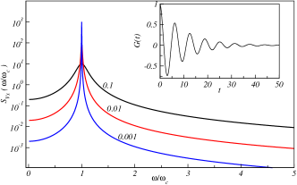
Figure 1: (Color online) Power spectral density $S_{v_{x}}(\omega)=S_{v_{y}}(\omega)$, Eq. (3), for $kT/m=1$, $\omega_{c}=1$ and different $\gamma$ (reported in the legend). Inset shows the velocity correlation function of Eq. (4), $G(t)$, for $\gamma=0.1$.

II Unbounded electron gas

In an equilibrium neutral plasma electrons of charge $q$ and mass $m$ oscillate with characteristic angular frequency chen_plasma $\omega_{p}=[n_{0}q^{2}/(m\varepsilon_{0})]^{1/2}$ (in S.I. notation), where $n_{0}$ is the average electron density and $\epsilon_{0}$ the vacuum permittivity. In the following we restrict ourselves to weakly magnetized plasmas to ensure that the cyclotron frequency associated with $B_{0}$, $\omega_{c}$, is much smaller than $\omega_{p}$, i.e., $\omega_{c}=qB_{0}/m\ll\omega_{p}$. This allows us to reduce the dynamics of a magnetoplasma electron to the 2D Brownian motion of a charged particle subjected to a uniform magnetic field. This is a longstanding problem in plasma and astroparticle physics magLE ; Garb ; additional_refs . Here we limit ourselves to introduce the results relevant to the discussion of our simulation data.

The corresponding Langevin equation reads

$$\vec{v}=\dot{\vec{r}},$$

$$\dot{\vec{v}}=\frac{q}{m}(\vec{v}\times\vec{B}_{0})-\gamma\vec{v}+\sqrt{2\gamma\frac{kT}{m}}~{}\vec{\xi}(t),$$ (1)

where the vector $\vec{\xi}(t)=(\xi_{x}(t),\xi_{y}(t))$ represents two independent Gaussian white noises with $\langle\xi_{i}(t)\rangle=0$ and $\langle\xi_{i}(t)\xi_{i}(0)\rangle=\delta(t)$ for $i=x,y$.

For numerical purposes, it is convenient to rescale both time, $t\to\omega_{c}t$, and space, $r\to r/\lambda$. We recall that $\omega_{c}$ is the $B_{0}$-dependent cyclotron angular frequency and $\lambda$ is the $T$-dependent electron gyroradius $\lambda=\sqrt{kT/(m\omega_{c}^{2})}$ chen_plasma . In dimensionless units Eq. (II) reads

$$\dot{\vec{r}} = \vec{v},$$

$$\dot{\vec{v}} = \vec{v}\times\vec{b}_{0}-g\vec{v}+\sqrt{2g}\vec{\xi}(t),$$ (2)

where $\vec{b}_{0}$ is a unity vector parallel to $\vec{B}_{0}$. Note that, in the absence of boundaries, the only free parameter in the dimensionless Langevin equation (II) is the scaled damping constant $g=\gamma/\omega_{c}$. In the foregoing sections all results will be given in dimensional units for reader’s convenience.

For the linear and unconstrained dynamics of Eq. (II) the p.s.d. $S(\omega)=\langle|\hat{\vec{r}}(\omega)|^{2}\rangle$, with $\hat{\vec{r}}(\omega)$ standing for the Fourier transform of $\vec{r}(t)$, can be computed analytically by means of standard harmonic analysis Gard ; HT82 . Taking advantage of the fact that $\xi_{x}(t)$ and $\xi_{y}(t)$ are uncorrelated white Gaussian noises, we obtain

$$S_{x}(\omega) = S_{y}(\omega)=\frac{S_{v_{x}}}{\omega^{2}},$$ (3)

$$S_{v_{x}}(\omega) = \frac{2kT}{m}\frac{\gamma(\omega^{2}+\gamma^{2})(\omega^{2}+\gamma^{2}+\omega_{c}^{2})}{\gamma^{2}\left(\omega^{2}+\gamma^{2}+\omega_{c}^{2}\right)^{2}+\omega^{2}\left(\omega^{2}+\gamma^{2}-\omega_{c}^{2}\right)^{2}},$$

where $S_{i}$ and $S_{v_{i}}$ denote the p.s.d. of the $i=x,y$ components of the 2D vectors $\vec{r}$ and $\vec{v}$, respectively. Note that at resonance $\omega=\omega_{c}$, the peak of the transverse velocity is $S_{v_{x}}(\omega_{c})=v^{2}_{\rm th}/(2\gamma)$, with $v_{\rm th}^{2}=\langle{\vec{v}}^{\;2}\rangle=2kT/m$. In view of the discussion below, we recall here that the stationary autocorrelation function of the velocity, $G(t-t^{\prime})=\langle v_{x}(t)v_{x}(t^{\prime})\rangle=\langle v_{y}(t)v_{y}(t^{\prime})\rangle$, solely depends on the difference $t-t^{\prime}$ and is related to the inverse Fourier transform of the p.s.d. $S_{v_{x}}(\omega)$ through the Wiener-Khinchin theorem Garb ; additional_refs ; Gard ; HT82 ,

$$G(t-t^{\prime}) = \langle v_{x}(t)v_{x}(t^{\prime})\rangle=\frac{1}{2\pi}\int_{-\infty}^{\infty}S_{v_{x}}(\omega)e^{i\omega(t-t^{\prime})}\,d\omega$$ (4)

$$= \frac{kT}{m}e^{-\gamma\mid t-t^{\prime}\mid}\cos{[\omega_{c}(t-t^{\prime})]}.$$

For an unbounded planar electron gas, the stationary distribution density of the velocity is Maxwellian magLE ; Garb ; additional_refs and does not depend on either the damping constant, $\gamma$, or the magnetic field, $B_{0}$,

$$f(\vec{v})=\frac{m}{2\pi kT}\exp{\left(-\frac{m\vec{v}\,^{2}}{2kT}\right)}.$$ (5)

The autocorrelation function of the electron coordinates, $\langle\vec{r}(t)\vec{r}(t^{\prime})\rangle$, diverges as a function of $t$ and $t^{\prime}$ because the free motion of electrons on the plane is unbounded.

To this regard it should be noticed that the diffusion of a Brownian charge carrier on a plane perpendicular to a constant magnetic field is normal, that is, for asymptotically large $t$, $\langle\vec{r}\,^{2}\rangle=4D_{B}t$ with

$$D_{B}=\frac{kT}{m\gamma}~{}\frac{\gamma^{2}}{\gamma^{2}+\omega_{c}^{2}}.$$ (6)

This means that for $B_{0}>0$ the particle diffusivity gets suppressed, as $D_{B}$ is smaller than the free diffusion coefficient $D_{0}=kT/(m\gamma)$.

The typical velocity p.s.d., $S_{v_{x}}(\omega)$, and an example of velocity autocorrelation function, $G(t)$, are depicted in Fig. 1 for different values of the damping constant $\gamma$. The peak at the cyclotron frequency $\omega_{c}$ broadens as $\gamma$ is increased. In the remaining sections of this paper we choose $\gamma$ to be much smaller than $\omega_{c}$, i.e. $\gamma\ll\omega_{c}$: This ensures that the cyclotron peak is well pronounced or, equivalently, that electrons with any given velocity $v$ tend to perform many cyclotron orbits of radius $r_{c}=v/\omega_{c}$, before being perturbed by the combined action of noise and friction. Accordingly, in the underdamped limit the diffusion coefficient $D_{B}$ tends to $kT\gamma/(m\omega_{c}^{2})=\lambda^{2}\gamma$.

III Finite systems

Our goal now is to compute the power spectral densities (p.s.d.), $S(\omega)$, of a confined 2D gas of electrons with finite temperature and for different geometries and boundary conditions. It should be noticed that $S(\omega)$ encodes important information about the electromagnetic transmission properties of the electron gas. In fact, $S(\omega)$ can be directly linked to the imaginary part of the gas electric susceptibility, $\kappa(\omega)$, via the fluctuation-dissipation relation, $S(\omega)\sim kT{\rm Im}[\kappa(\omega)]$ sosenko94 .

We start with the simplest case of an electron gas trapped in a strip delimited by two walls parallel to the $y$ axis and a fixed distance $d$ apart. Electrons are assumed to be reflected elastically by the strip boundaries, which leads to a zero net transverse flux in the $x$ direction.

We numerically integrated the dimensionless Langevin equation (II) for $g$ in the range $10^{-3}\div 10^{-2}$ and then restored dimensional units with $\omega_{c}=1$ and fixed system size. With respect to the time unit, this corresponds to reporting $\omega$ in units of $\omega_{c}$, with no severe restriction on the actual value of $B_{0}$, but for the condition that $\omega_{c}\ll\omega_{p}$ (see Secs. II and V for more details). With respect to the space units, setting the width of the strip to a given value, $d$, makes the electron p.s.d. depend explicitly on the temperature, which had been eliminated from Eq. (II) by expressing all lengths in units of $\lambda$. Note that in our plots $\omega_{c}=1$, so that the scaled temperature $kT/m$ boils down to the square of the gyroradius, $\lambda$, introduced in Sec. II.

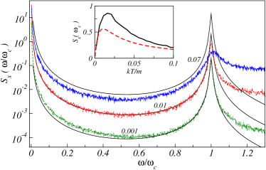
Figure 2: (Color online) Transverse power spectral density, $S_{x}(\omega)$, of an electron moving in a strip of width $d=1$ (see sketch in Fig. 3), as computed from Eq. (II) for $\gamma=0.005$, $\omega_{c}=1$ and the scaled temperature $kT/m$ reported in the legend. Solid curves represent the corresponding p.s.d. for an unbounded planar system. Inset: amplitude of the cyclotron peak $S_{x}(\omega_{c})$ as a function of $kT/m$ (solid curve) and its analytical approximation, Eq. (8) (dashed curve). Note that for $\omega_{c}=1$ the scaled temperature $kT/m$ coincides with $\lambda^{2}$.

III.1 Resonant cyclotron peak

The typical p.s.d. of the transverse coordinate, $S_{x}(\omega)$, are depicted in the main panel of Fig. 2. The finely dotted curves represent $S_{x}(\omega)$, as computed numerically through Eq. (II) with $\gamma=0.005$ and ideal reflecting boundaries located at $x=\pm d/2$ with $d=1$. The solid curves are the corresponding $S_{x}(\omega)$ for an unbounded planar electron gas, as predicted in Eq. (3). The height as well as the width of the cyclotron peak depend on the scaled temperature $kT/m$.

Unlike for the case of an infinite system, the amplitude of the cyclotron peak, $S_{x}(\omega_{c})$, for the confined electron gas depends resonantly on the temperature, as shown in the inset of Fig. 2: As $T$ is gradually increased, $S_{x}(\omega_{c})$ goes through a maximum for an optimal temperature, $T_{c}$, whose dependence on the confinement geometry is investigated in the following sections. This behavior may be reminiscent of stochastic resonance SR . However, we anticipate that here the optimal temperature is defined by the matching of two length scales, rather than two time scales, as it is the case in ordinary stochastic resonance SR ; JH91 . Finite volume effects have been reported in the early stochastic resonance literature phi4 , but in a totally different context.

III.2 Quantitative interpretation

The resonant temperature dependence of the cyclotron peak can be qualitatively explained as follows. First we recall that, in the underdamped regime, the diffusion time of a charged Brownian particle across a strip of width $d$ is strongly suppressed by the presence of a magnetic field, especially for $\gamma t\ll 1$. From Eq. (43) of Ref. Garb , $\langle\vec{r}\,^{2}\rangle={\cal{O}}(t^{3})$; hence, the transverse diffusion time in the strip can be safely assumed to be much shorter than the cyclotron period, as illustrated in panels (a) and (b) of Fig. 3.

Then, we notice that, as the interaction of the electrons with the walls is elastic, the equilibrium distribution of their velocity is not affected by the boundary geometry and is still given by the Maxwell distribution of Eq. (5).

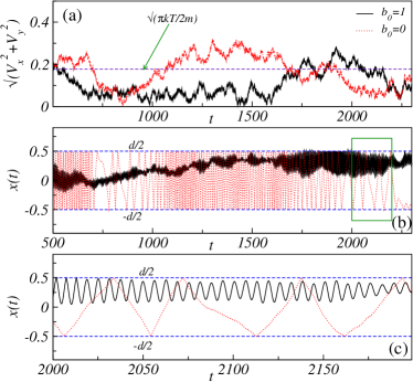
Figure 3: (Color online) Trajectory samples of $|\vec{v}|(t)$, (a), and $x(t)$, (b)-(c), for $kT/m=0.02$, $\gamma=10^{-3}$, $d=1$ and $\omega_{c}=1$ (black curves) or $B_{0}=0$ (red curves). In (c) is a blow-up of the trajectory portion marked by a rectangle in (b) The horizontal dashed line in (a) represents $\langle|\vec{v}|\rangle$ as computed from Eq. (7).

Moreover, the cyclotron radius of an electron moving with instantaneous velocity $v$ is $r_{c}=v/\omega_{c}$; in the regime of low damping, $\gamma\ll\omega_{c}$, we can neglect the effects of friction on the electron orbits. This means that the contribution to $S_{x}$ from a circular orbit of constant radius $r_{c}$ is proportional to $r_{c}^{2}/2\gamma$ [see discussion following Eq. (3)], that is, increases quadratically with $v$. However, this conclusion applies only to electronic trajectories with centers located a distance not smaller than $r_{c}$ away from the reflecting boundaries. Indeed, when the electrons come too close to the boundaries, they repeatedly bounce off the walls, so that their trajectories get distorted [see Fig. 3(c)]. For an equilibrium distribution of the electron velocities, this surely happens when their orbit diameter is larger than half the strip width, $2r_{c}>d/2$.

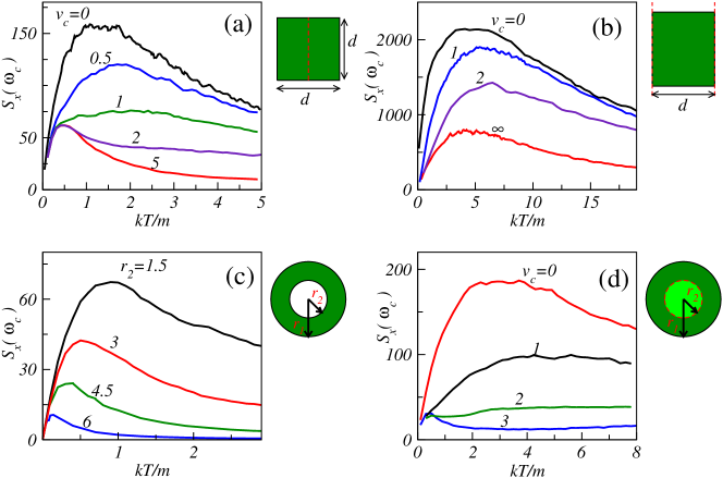
Figure 4: (Color online) Amplitude of the cyclotron peak, $S_{x}(\omega_{c})$, as a function of the scaled temperature $kT/m$ for the different geometries of Sec. IV as sketched. In all four panels $\omega_{c}=1$ and $\gamma=0.00166$ (a), (b) and $0.003$ (c), (d). (a) Square box containing a semi-transparent wall $x=h$ [case (i)]. Simulation parameters are: $d=12$, $h=0$, and threshold velocity $v_{c}$ as reported next to the relevant data sets. (b) [case (ii)] Infinite strip with semi-transparent walls. Simulation parameters are: $d=18$ and $v_{c}$ as reported next to the relevant data sets. (c) Annulus with reflective inner boundary [case (iii)] with $v_{c}=\infty$. The outer radius is kept constant, $r_{1}=9$, and the inner radius, $r_{2}$, varied as in the legend. (d) [case (iv)] Same geometry as in (c) but with constant inner radius, $r_{2}=4.5$, and semi-transparent inner wall with threshold velocity, $v_{c}$, in the legend.

In view of the arguments above, we assume for simplicity that fast electrons with too large a cyclotron radius, say, $r_{c}>d/4$, do not contribute to the cyclotron peak, whereas only a fraction $1-4r_{c}/d$ of the slower electrons with $r_{c}<d/4$ do. On further noticing that from Eq. (5) the equilibrium distribution of $v$ is

$$\rho(v)=\frac{mv}{kT}\exp{\left(-\frac{mv^{2}}{2kT}\right)}\,,$$ (7)

we obtain the following estimate for the amplitude of the cyclotron peak,

$$S_{x}(\omega_{c})\simeq\frac{(\bar{T}d)^{2}}{32\gamma}\left[2+e^{-\frac{1}{2\bar{T}^{2}}}-3\sqrt{\frac{\pi}{2}}\,\bar{T}\,{\rm Erf}\left(\frac{1}{\sqrt{2\bar{T}^{2}}}\right)\right],$$ (8)

where ${\bar{T}}=4\sqrt{kT/m}/(d\omega_{c})$ and Erf($\dots$) denotes the standard error function. Note that this estimate for $S_{x}(\omega_{c})$ systematically underestimates the corresponding simulation curve as we neglected the residual contribution from electronic orbits larger, but not too larger, than $d/4$. By numerically evaluating Eq. (8), one concludes that both the resonance value of the cyclotron peak, $S_{\rm max}(\omega_{c})$, and $T_{c}$ grow quadratically with $d$, namely, $kT_{c}/m\simeq 0.01(\omega_{c}d)^{2}$ and $S_{\rm max}(\omega_{c})\simeq 2.8\cdot 10^{-3}d^{2}/\gamma$.

We also stress that the emergence of a resonant cyclotron peak is not conditioned by the elastic boundary assumption. Boundary randomness or fluctuations may, indeed, affect the residual contribution from large electronic orbits with $r_{c}>d/4$, but not the bulk contribution estimated in Eq. (8).

IV Dependence on geometry and boundary conditions

Next we numerically compute $S_{x}(\omega_{c})$ as a function of the temperature for different geometries and boundary conditions, in order to demonstrate the robustness of the temperature resonance of the cyclotron peak.

We consider here three confining setups for the 2D electron gas:

(i) Box with internal semi-transparent wall.
Consider a $d\times d$ square box, centered at the origin $x=y=0$, and containing a semi-transparent internal wall, $x=h$ with $|h|<d/2$, parallel to the $y$ axis. The internal wall acts like a porous filter letting charges pass through only if the $x$ component of their velocity, $v_{x}$, is larger than a certain threshold velocity $v_{c}$, i.e. $v_{x}>v_{c}$. If $v_{x}\leq v_{c}$, the electrons are elastically reflected back into their half box. We fix $d=12$, $h=0$ and plot in Fig. 4(a) the amplitude of the cyclotron peak as a function of the scaled temperature $kT/m$ for different values of the threshold. For $v_{c}=0$ the compartment wall is transparent, so that the effective width of the box is $d$, whereas for $v_{c}>5$ the internal wall acts as an almost perfectly reflective boundary, thus dividing the square box in two rectangular compartments of width $d/2$. Despite the different geometries, confined cyclotron orbits are confirmed to generate a resonant temperature dependence of the electronic p.s.d., no matter what $v_{c}$. Moreover, in agreement with our analytical discussion of the infinite strip from Sec. III.2, the optimal temperature $T_{c}$, corresponding to the maxima of the plotted curves, diminishes with, $d^{2}\longrightarrow d^{2}/4$, by a factor $4$ on increasing $v_{c}$ from $0$ to $\infty$ and, thus, halving the container width.

(ii) Infinite strip with semi-transparent walls.
Let us consider the infinite strip of Sec. III.1 with the important difference that now its parallel walls are semi-transparent, as described in $(i)$. If $v_{x}\leq v_{c}$ the electrons are contained in the strip; if $v_{x}>v_{c}$ the electrons exit one wall and reenter through the other one with periodic boundary conditions. In Fig. 4(b), the peak amplitude $S(\omega_{c})$ is plotted as a function of the temperature for different values of the threshold. Since the boundaries are periodic for $v_{c}=0$ and reflective for $v_{c}=\infty$, here our approximate estimate for $S(\omega_{c})$ from Sec. III.2 is expected to work well only as $v_{c}\to\infty$. In this limit, Eq. (8) reproduces fairly closely both $T_{c}$ and $S_{\rm max}(\omega_{c})$. In the opposite limit of purely periodic boundary conditions, the cyclotron peak at resonance, $S_{\rm max}(\omega_{c})$, gets enhanced, while $T_{c}$ only weakly depends on $v_{c}$.

(iii) Annulus with with a reflecting inner wall and (iv) with a semi-transparent inner wall.
Next let the electrons be trapped in a circle with radius $r_{1}$, which represent an ideal reflecting boundary. The inner space is divided by a second circle of radius $r_{2}$, with $r_{2}<r_{1}$, into two compartments. The inner circle is concentric with the outer circle and its circumference works as a semi-transparent wall (case (iv)) with threshold velocity $v_{c}$ (applied to the radial component of ${\vec{v}}$). The case (iii) of an ideal reflecting inner circle, corresponds to setting the threshold velocity $v_{c}=\infty$, see Fig. 4(c), the gas is confined to an annulus. As one can anticipate from the discussion in Sec. III.2, the maximum of the cyclotron peak, $S_{\rm max}(\omega_{c})$, decreases on increasing $r_{2}$, see Fig. 4(c). Correspondingly, the optimal temperature, $T_{c}$, also decreases because the width of the annulus shrinks. The dependence of the resonant cyclotron effect on $v_{c}$ is illustrated in Fig. 4(d). The effect is most pronounced in the case of a perfectly transparent inner circle, $v_{c}=0$. Indeed, lowering $v_{c}$ enlarges the surface accessible to the cyclotron orbits of the confined electrons. As suggested by Eq. (8), $T_{c}$ and the maximum of $S(\omega_{c})$ grow quadratically with the effective transverse dimensions of the gas container; for the simulation parameters reported in Fig. 4(d), this corresponds to an increase of both quantities by a factor of about $4$ as $v_{c}$ raises from $0$ to $\infty$.

(v) Infinite strip with internal semi-transparent wall.
Finally, we show that by appropriately choosing the geometry of the system, the cyclotron peak can go through two maxima as a function of temperature. Such a double resonance was found by inserting an internal wall, $x=h$ with $|h|<d/2$, of tunable threshold $v_{c}$ in the infinite strip of Sec. III.1. Our simulation results for a symmetric geometry with $d=12$, $h=0$ and different $v_{c}$ are displayed in Fig.  5(a). The limiting regimes, $v_{c}=0$ and $v_{c}\to\infty$ are well reproduced by our approximate formula in Eq. (8). In the intermediate regimes, say at $v_{c}=2$, the $S(\omega_{c})$ features two maxima. The low temperature maximum is centered around the optimal temperature, $T_{c}^{(\infty)}$, corresponding to a partitioned strip, $v_{c}=\infty$. Most remarkably, the optimal temperature of the second maximum on the right is systematically higher than the optimal temperature, $T_{c}^{(0)}$, of the un-partitioned strip, $v_{c}=0$. Moreover, such a double resonance could only be found for certain combinations of $v_{c}$ and $h/d$, as shown in Fig. 5(b).

The occurrence of a double resonance can be explained by noticing that for electrons with $v_{x}\leq v_{c}$, the wall acts as an effective partition. In Fig. 5(a), where $h=0$, this corresponds to splitting the strip into two equal strips of half width. Correspondingly, the slow electrons trapped in either half strip contribute a cyclotron peak that is the highest for $T\simeq T_{c}^{(\infty)}$. Fast electrons with $v_{x}>v_{c}$ are free to move across the full width of the strip, so that the optimal temperature of their cyclotron orbits ought to approach $T_{c}^{(0)}$ with $T_{c}^{(0)}\simeq 4T_{c}^{(\infty)}$. However, by taking a closer look at our derivation of Eq. (8), it is apparent that in the case of fast electrons the lower limit of the integral must be modified to account for the condition $v_{x}>v_{c}$. As a consequence of the bell shaped profile of the Maxwell distribution, such a modification of the integration range moves the optimal value $\bar{T}_{c}$ to appreciably higher values, in agreement with Fig. 5.

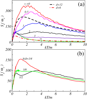
Figure 5: (Color online) Amplitude of the cyclotron peak, $S_{x}(\omega_{c})$, as a function of the scaled temperature $kT/m$ [case (v) of Sec. IV] for $\omega_{c}=1$ and $\gamma=0.00166$. (a) Infinite strip of width $d=12$ with a semi-transparent filter located at $h=0$ and different thresholds $v_{c}$ (in the legend). The curves of Eq. (8) for $d=12$ (dashed) and $6$ (dotted-dashed) are reported for a comparison; (b) Geometry as in (a), $v_{c}=2$ and different $h$ (in the legend).

V Concluding remarks

The temperature controlled resonance of the cyclotron spectra, emerging from a matching between the system size length $d$ with the thermal electron gyroradius $\lambda$, becomes detectable for a confined magnetized gas of charged particles under two important conditions, summarized by the inequalities $\gamma\ll\omega_{c}\ll\omega_{p}$. The condition $\omega_{c}\ll\omega_{p}$, introduced in Sec. II, required applying magnetic fields of relatively low intensity. The underdamped regime, $\gamma\ll\omega_{c}$, was assumed to enhance the cyclotron peak of the transverse p.s.d., $S_{x}(\omega)$, over its background. Both conditions can be met in magnetoplasmas gentle_plasma .

In normal metals the observation of the resonant cyclotron effects reported here might seem out of question. At room temperature typical values of the electron damping constant are $\gamma\sim 10^{13}$ s^-1, or larger, so that an underdamped electron dynamics would set on only for exceedingly large magnetic field Abri . A more promising playground for an experimental demonstration of the effect under investigation is a 2D electron gas, where mobility can be quite high, thus, corresponding to a small damping constant, $\gamma\sim 10^{9}$ s^-1. A relatively low magnetic fields (of about $0.1$ T) then would easily satisfy the condition $\gamma\ll\omega_{c}$. However, since the plasma frequency, $\omega_{p}$, of an unconstrained 2D electron gas tend to be very low, artificial geometries should be implemented. To this regard it helps mentioning two sets of recent experiments, which detected, respectively, oscillations in the magnetoresistances of two-dimensional lateral surface superlattices with square patterns long , and dynamical phase transitions between localized and superdiffusive (or ballistic) regimes for paramagnetic colloidal systems confined to magnetic bubble domains tierno . Both results can be explained, in semiclassical approximation, as a commensurability effect between the cyclotron radius of the magnetocharges and the spatial periodicity of the substrate, without the need to invoke quantum mechanics.

We finally point out that the diffusion of confined magneto-charged particles is a topic of increasing interest not only in solid state physics. In medical research, for instance, magnetic nanostructures confined to 2D geometries are thought to offer the most exciting avenues to nanobiomagnetic applications, including targeted drug delivery, bioseparation and cancer therapy, even if their diffusion properties are not yet fully controllable. The possibility of extending our analysis to nanobiomagnetic processes at the cellular level requires advances on at least two issues: (1) diffusion of complex magnetic materials. In biomedical applications, pointlike magneto-charges are often replaced by synthetic magnetic structures, such as magnetic microdiscs with a spin-vortex ground state medicine ; (2) walls interactions. Contrary to our simple model, the interactions between a magneto-charge and cellular walls are typically inelastic, namely characterized by finite interaction times, energy transfer and even structural changes, like the activation on mechanosensitive ion channels. Both issues are the subject of ongoing investigations by research teams worldwide.

- (1) K. W. Gentle, Rev. Mod. Phys. 67, 809 (1995).
- (2) P. P. Sosenko, Phys. Scripta 50, 82 (1994).
- (3) I. Li and L. Jeng-Mei, Phys. Rev. Lett. 74, 3161 (1995).
- (4) L. Gammaitoni, P. Hänggi, P. Jung, and F. Marchesoni, Rev. Mod. Phys. 70, 223 (1998).
- (5) P. S. Burada, P. Hänggi, F. Marchesoni, G. Schmid, and P. Talkner, ChemPhysChem 10, 45 (2009).
- (6) P. K. Ghosh, F. Marchesoni, S. E. Savel’ev, and F. Nori, Phys. Rev. Lett. 104, 020601 (2010).
- (7) P. P. Miller, A. F. Vandome, and J. McBrewster, Electron Cyclotron Resonance (Mauritius, Alphascript, 2010).
- (8) F. F. Chen, Introduction to Plasma Physics (Plenum Press, New York and London, 1974).
- (9) J. B. Taylor, Phys. Rev. Lett. 6, 262 (1961); B. Kurşunoǧlu, Phys. Rev. 132, 21 (1963).
- (10) R. Czopnik and P. Garbaczewski, Phys. Rev. E 63, 021105 (2001).
- (11) J. I. Jiménez-Aquino and M. Romero-Bastida, Phys. Rev. E 74, 041117 (2006); I. Holod, A. Zagorodny, and J. Weiland, Phys. Rev. E 71, 046401 (2005); T. P. Simoẽs and R. E. Lagos, Physica A 355, 274 (2005); L. Ferrari, Physica A 163, 596 (1990).
- (12) C. W. Gardiner, Handbook of Stochastic Methods (Springer, Berlin, 2004).
- (13) P. Hänggi and H. Thomas, Phys. Rep. 88, 207 (1982).
- (14) P. Jung and P. Hänggi, Phys. Rev. A 44, 8032 (1991).
- (15) F. Marchesoni, L. Gammaitoni, and A.R. Bulsara, Phys. Rev. Lett. 76, 2609 (1996).
- (16) A. A. Abrikosov, Fundamentals of the Theory of Metals (North-Holland, Amsterdam, 1988).
- (17) D. E. Grant, A. R. Long, and J. H. Davies, Phys. Rev. B 61, 13127 (2000); S. Chowdhury, C. J. Emeleus, B. Milton, E. Skuras, A. R. Long, J. H. Davies, G. Pennelli, and C. R. Stanley, Phys. Rev. B 62, R4821 (2000).
- (18) P. Tierno, T. H. Johansen, and T. M. Fischer, Phys. Rev. Lett. 99, 038303 (2007); P. Tierno, A. Soba, T. H. Johansen, and F. Saguès, Appl. Phys. Lett. 93, 214102 (2008).
- (19) D. H. Kim, E. A. Rozhkova, I. V. Ulasov, S. D. Bader, T. Rajh, M. S. Lesniak, and V. Novosad, Nature Mat. 9, 165 (2010).