INR-TH-2011-10

Non-Gaussianity of scalar perturbations
generated by conformal mechanisms

M. Libanov, S. Mironov, V. Rubakov

Institute for Nuclear Research of the Russian Academy of Sciences,
60th October Anniversary Prospect, 7a, 117312 Moscow, Russia;
Physics Department, Moscow State University
Vorobjevy Gory, 119991, Moscow, Russia

Abstract

We consider theories which explain the flatness of the power spectrum of scalar perturbations in the Universe by conformal invariance, such as conformal rolling model and Galilean Genesis. We show that to the leading non-linear order, perturbations in all models from this class behave in one and the same way, at least if the energy density of the relevant fields is small compared to the total energy density (spectator approximation). We then turn to the intrinsic non-Gaussianities in these models (as opposed to non-Gaussianities that may be generated during subsequent evolution). The intrinsic bispectrum vanishes, so we perform the complete calculation of the trispectrum and compare it with the trispecta of local forms in various limits. The most peculiar feature of our trispectrum is a (fairly mild) singularity in the limit where two momenta are equal in absolute value and opposite in direction (folded limit). Generically, the intrinsic non-Gaussianity can be of detectable size.

1 Introduction

Scalar perturbations in the Universe may well originate from inflation [1]. In that case, approximate flatness of their power spectrum is due to the approximate de Sitter symmetry of inflating background. As pointed out in Ref. [2], a possible alternative to the de Sitter symmetry in this context is conformal invariance. Concrete models employing conformal invariance, instead of the de Sitter symmetry, for explaining the flat scalar spectrum include conformal rolling [3] and Galilean Genesis [4]. Despite substantially different motivations and dynamical features, the latter models end up in one and the same mechanism that generates scalar perturbations. From this prospective, the theory boils down to a model with two scalar fields $\rho$ and $\Theta$ and the Lagrangian

$$L=L_{\rho}+\frac{1}{2}\rho^{2}\left(\partial_{\mu}\Theta\right)^{2}\;,$$ (1)

where $L_{\rho}$ governs the dynamics of $\rho$. Under scaling transformations, the field $\rho$ scales as $\rho(x)\to\lambda\rho(\lambda x)$; it provides for a non-trivial background $\rho_{c}$. The field $\Theta$ scales as $\Theta(x)\to\Theta(\lambda x)$; the perturbations of the field $\Theta$ serve as predecessors of the adiabatic perturbations. One makes sure that at the time the perturbations of $\Theta$ are generated, gravitational effects on the dynamics of the two fields are irrelevant (this is achieved in different ways in Ref. [3] and Ref. [4]) and assumes that the background field $\rho_{c}$ is spatially homogeneous. Then conformal invariance of the field equation for $\rho$ implies that

$$\rho_{c}(x_{0})=-\frac{1}{x_{0}}\;,\;\;\;\;\;\;x_{0}<0\;,$$ (2)

where $x_{0}=\eta$ is conformal time in the conformal rolling model and $x_{0}=t$ is cosmic time in the Galilean Genesis scenario. In such a background, the field $\Theta$ behaves exactly in the same way as massless scalar field (minimally coupled to gravity) in the de Sitter space-time. The modes of its perturbations about a certain background value $\bar{\Theta}$,

$$\theta(x)=\Theta(x)-\bar{\Theta}\;,$$

start off in the WKB regime and freeze out when $k|x_{0}|\sim 1$, where $k$ is (conformal) momentum. Assuming that the field $\theta(x)$ is originally in its vacuum state, one obtains, at the linearized level, the flat power spectrum of the Gaussian field $\theta({\bf k})$ at late times111Deviation from exact conformal invariance naturally gives rise to the tilt in the power spectrum, see, e.g., Ref. [5]., when $k|x_{0}|\ll 1$. The conformal stage ends up at some point, and the $\theta$-perturbations are reprocessed into adiabatic ones at much later epoch via, e.g., curvaton [6] or modulated decay [7] mechanism.

A common feature of the conformal models of Refs. [3, 4] is the existence of the perturbations of the field $\rho$ about the background (2). The Lagrangian $L_{\rho}$ contains a small parameter, call it $h$, then $\delta\rho\propto h$ ($h^{2}$ is quartic self-coupling in the conformal rolling model; we relate the parameter $h$ to the parameters of the galileon Lagrangian in the Galilean Genesis scenario in Section 2.1, see Eq. (9)). As discussed in Refs. [3, 4], the perturbations $\delta\rho$ have rather peculiar properties. Nevertheless, as we review in Section 2.1, these perturbations are exactly the same (modulo overall amplitude) in the two, apparently very different models. Furthermore, in Section 2.2 we give a general argument showing that the properties of the linearized perturbations $\delta\rho$ are common to a large class of models employing conformal invariance.

There is a subtlety here. Strictly speaking, our observation is valid in a theory without gravity or in the case when the energy density of the field $\rho$ is small compared to the total energy density in the Universe (spectator approximation). Though is is likely that our results are valid in much more general setting, the corresponding analysis is yet to be done. We proceed in this paper by neglecting gravity altogether.

So, it is of interest to study the effects of the perturbations $\delta\rho$ on the field $\theta$ and, in the end, on the adiabatic perturbations. There are at least two of these effects, namely, the statistical anisotropy and non-Gaussianity. Of course, the non-Gaussianity may well be generated also at the time the $\theta$-perturbations are converted into the adiabatic ones. In this respect the conformal models are nothing special as compared to inflationary theories equipped with the curvaton or modulated decay mechanism; for this reason we are going to disregard this conversion-related non-Gaussianity. What we are interested in is the intrinsic non-Gaussianity, which is due to the interaction of the field $\theta$ with perturbations $\delta\rho$.

The resulting phenomenology depends strongly on what happens to the field $\theta$ after the conformal stage (2) ends up. One option is that the field $\theta({\bf k})$ starts evolving again, and its evolution proceeds until it becomes superhorizon in the conventional sense. This option is fairly natural in the conformal rolling model of Ref. [3] and more contrived in the Galilean Genesis222In the context of the Galilean Genesis, an intermediate stage of the evolution of $\theta$ may occur provided that the effective scale factor $\rho(\pi)$ is a non-trivial function of the galileon field $\pi$, such that $\rho\propto{\rm e}^{\pi}$ at $\pi$ smaller than some value $\pi_{0}$ and $\rho=\mbox{const}$ at $\pi>\pi_{0}$. Then the field $\theta$ feels the background (2) at early times, when $\pi<\pi_{0}$, and temporarily gets frozen out when $k|x_{0}|\sim 1$, as discussed in the text. If the opposite regime $\pi>\pi_{0}$ sets in later, but still at some sufficiently early time when the space-time is nearly Minkowskian, the field $\theta({\bf k})$ indeed starts to oscillate again at that time. These oscillations terminate when the Hubble parameter becomes large enough and the field $\theta({\bf k})$ exits the horizon. of Ref. [4]. Both statistical anisotropy and non-Gaussianity generated in this case are studied in Ref. [8].

Here we consider the opposite case, i.e., we assume that the field $\theta$ does not evolve after the end of the conformal stage. This option is particularly natural in the Galilean Genesis, but it is not contrived in the conformal rolling scenario either. In models from this sub-class, the adiabatic perturbations inherit the statistical properties of $\theta$-perturbations that exist already at the late conformal stage, when $k|x_{0}|\ll 1$. The statistical anisotropy in the field $\theta$ is induced by long-ranged perturbations $\delta\rho$. This effect has been studied in Ref. [9] with the result that the leading statistical anisotropy in the power spectrum of $\theta$, and hence of adiabatic perturbation $\zeta$, has the quadrupole form,

$${\cal P}_{\zeta}({\bf k})={\cal P}_{0}(k)\left(1+c_{1}\cdot h\cdot\frac{H_{0}}{k}\cdot\frac{{k}_{i}{k}_{j}}{k^{2}}w_{ij}-c_{2}\cdot h^{2}\cdot\frac{({\bf ku})^{2}}{k^{2}}\right)\;,$$

where ${\cal P}_{0}(k)$ is isotropic (and nearly flat) power spectrum obtained at the linearized level, $u_{i}$ and $w_{ij}$ are unit 3-vector and unit traceless 3-tensor of a general form, $H_{0}$ is the present value of the Hubble parameter, the parameter $c_{1}$ is of order 1 and $c_{2}$ is positive and logarithmically enhanced.

The main purpose of this paper is to study the intrinsic (as opposed to conversion-related) non-Gaussianity in this sub-class of models. In the absence of the cubic self-interaction of the field $\theta$, the intrinsic bispectrum vanishes, so we have to consider the intrinsic trispectrum. Perhaps the most striking feature of the trispectrum is the singularity in the limit where two momenta are equal in absolute value and have opposite directions (folded limit, in nomenclature of Ref. [10]). The singular part of the connected four-point function has been calculated in our earlier paper [11] with the result

$\displaystyle\langle\zeta_{\mathbf{k}_{1}}\zeta_{\mathbf{k}_{2}}\zeta_{\mathbf{k}_{3}}\zeta_{\mathbf{k}_{4}}\rangle=\mbox{const}$ $\displaystyle\cdot\delta\left(\sum\limits_{i=1}^{n}\mathbf{k}_{i}\right)\cdot\frac{1}{k_{12}k_{1}^{4}k_{3}^{4}}\left[1-3\left(\frac{\mathbf{k_{12}k_{1}}}{k_{12}k_{1}}\right)^{2}\right]\left[1-3\left(\frac{\mathbf{k_{12}k_{3}}}{k_{12}k_{3}}\right)^{2}\right]$ (3)
$\displaystyle\mathbf{k_{12}}$ $\displaystyle=\mathbf{k_{1}}+\mathbf{k_{2}}\to 0\;,$

i.e., the trispectrum blows up as $k_{12}^{-1}$. This is in contrast to trispectra obtained in single-field inflationary models [10, 12, 13, 14, 15], and, indeed, there are general arguments [13] showing that in these models, the four-point function is finite in the limit $k_{12}\to 0$. The singularity in the four-point function (3) is due to the enhancement of the perturbations $\delta\rho$ at low momenta, see the discussion of the infrared properties of the conformal models in Ref. [9]. We will see in Section 3.3 that the most relevant features of the trispectrum are captured by its singular part.

Whether the intrinsic non-Gaussianity dominates over the conversion-related one, and whether the former is detectable depends on both the underlying conformal model and the mechanism that converts the $\theta$-perturbations into the adiabatic ones. Generically, the linear order relationship between $\zeta$ and $\theta$ is $\zeta=r\theta/\bar{\Theta}$, where $r\lesssim 1$ is the dilution factor. With our normalization (1), (2), the power spectrum of $\theta$-perturbations is $\mathcal{P}_{\theta}=1/(4\pi^{2})$. The background value $\bar{\Theta}$ cannot be estimated in a model independent way. It can be as large as $\bar{\Theta}\sim 10^{4}$, so that the correct adiabatic amplitude is obtained at $r\sim 1$. This can be the case, e.g., in the Galilean Genesis model. In such a situation, the conversion-related non-Gaussianities induced by the curvation or modulated decay mechanism are fairly small ($f_{NL}$, $g_{NL}$ are roughly of order 1 [16, 17, 18, 19]). On the other hand, the size of the intrinsic non-Gaussianity $t_{NL}$ (see Eq. (38) for its definition) is governed by the amplitude of the perturbations $\delta\rho$, so that

$$t_{NL}\sim\frac{h^{2}}{4\pi^{2}{\cal P}_{\zeta}}\;,$$

see Eq. (39) for numerical coefficient. There is no general reason to expect that the parameter $h$ is particularly small, except for the mild requirement $h\ll 1$ ensuring the self-consistency of the conformal scenario. This shows that the intrinsic non-Gaussianity may well be dominant and detectable (say, $t_{NL}\gtrsim 10^{6}$), though it size cannot be predicted because of our ignorance of the value of the parameter $h$. The situation is more subtle in the conformal rolling model; we consider this point in Section 3.3 with the result that dominant and detectable intrinsic non-Gaussianity is possible, but not generic.

This paper is organized as follows. To set the stage, we consider in Section 2.1 the linearized perturbations $\theta$ and $\delta\rho$ in the Galilean Genesis scenario and compare the resulting expressions with those obtained in the conformal rolling model. This Section contains nothing new as compared to Refs. [3, 4]; the main point is to show that the perturbations $\theta$ and $\delta\rho$ are identically the same in the two scenarios. In Section 2.2 we give a general argument showing that the properties of $\delta\rho$ are uniquely determined by conformal invariance (modulo the overall constant amplitude). Hence, the peculiarities of the adiabatic perturbations that we study in this paper, as well as the results of Refs. [9, 11], are common to the whole class of conformal mechanisms. We turn to the non-Gaussianity in Section 3, where we perform the complete calculation of the intrinsic trispectrum. We confirm our earlier result (3) concerning the singular part of the trispectrum. We then consider various limits, following the nomenclature of Refs. [10, 15], and compare them with local models [20, 21]. We conclude in Section 4. Some details of our calculations are collected in Appendix.

2 Perturbations in conformal scenarios

2.1 Galilean Genesis vs. conformal rolling

The galileon model has been introduced in Ref. [22]. The rolling galileon serves as the field $\rho$ entering (1) and (2). In the Minkowski space-time, the Lagrangian of the simplest conformally-invariant version [4] of the model is (mostly negative signature)

$$L_{\pi}=-f^{2}{\rm e}^{2\pi}\partial_{\mu}\pi\partial^{\mu}\pi+\frac{f^{3}}{\Lambda^{3}}\partial_{\mu}\pi\partial^{\mu}\pi\Box\pi+\frac{f^{3}}{2\Lambda^{3}}(\partial_{\mu}\pi\partial^{\mu}\pi)^{2}\;,$$ (4)

where $\Box=\partial_{\mu}\partial^{\mu}$. The field equation in Minkowski space-time admits the homogeneous solution $\pi_{c}$ such that

$${\rm e}^{\pi_{c}}=-\frac{1}{H_{*}x_{0}}\;,$$ (5)

where $x_{0}=t$ and

$$H_{*}^{2}=\frac{2\Lambda^{3}}{3f}\;.$$

Hence, one defines

$$\rho=H_{*}{\rm e}^{\pi}$$ (6)

so that the background solution is given by (2).

The quadratic action for perturbations about this solution is

$$S_{\delta\pi}=\frac{f^{2}}{H_{*}^{2}}\int~{}d^{4}x~{}\left\{\frac{1}{x_{0}^{2}}[(\partial_{0}\ {\delta\pi})^{2}-(\partial_{i}\ \delta\pi)^{2}]+\frac{4}{x_{0}^{4}}\delta\pi^{2}\right\}\;.$$

It is convenient to introduce the variable $\delta\rho=-x_{0}^{-1}\delta\pi$. It follows from (6) that $\delta\rho$ is the perturbation of the field $\rho$ about the background $\rho_{c}=-x_{0}^{-1}$. Its action reads

$$S_{\delta\rho}=\frac{2f^{2}}{H_{*}^{2}}\int~{}d^{4}x~{}\frac{1}{2}\left[(\partial_{0}\ {\delta\rho})^{2}-(\partial_{i}\ \delta\rho)^{2}+\frac{6}{x_{0}^{2}}(\delta\rho)^{2}\right]\;.$$

The field equation has a simple form,

$$\partial_{0}^{2}{\delta\rho}-\Delta\delta\rho-\frac{6}{x_{0}^{2}}\delta\rho=0\;.$$ (7)

Its properly normalized solution for given momentum ${\bf k}$ is

$$\delta\rho=h\cdot\mbox{e}^{i{\bf kx}}\cdot\frac{i}{4\pi}\sqrt{\frac{-t}{2}}H_{5/2}^{(1)}\left(-kx_{0}\right)\cdot\hat{B}_{\bf k}+h.c.\;,$$ (8)

where $\hat{B}^{\dagger}_{\bf k}$ and $\hat{B}_{\bf k}$ are creation and annihilation operators obeying the standard commutational relation $[\hat{B}_{\bf k},\hat{B}^{\dagger}_{\bf q}]=\delta({\bf k}-{\bf q})$, and

$$h=\frac{H_{*}}{\sqrt{2}f}\;.$$ (9)

The theory is weakly coupled in the relevant range of momenta provided that $h\ll 1$.

The mode (8) oscillates at early times, when $k|x_{0}|\gg 1$, while at late times it behaves as follows,

$$\delta\rho=h\cdot\mbox{e}^{i{\bf kx}}\cdot\frac{3}{4\pi^{3/2}}\frac{1}{k^{5/2}x_{0}^{2}}\cdot\hat{B}_{\bf k}+h.c.\;.$$

This behavior can be interpreted as local time shift [3, 4]. Indeed, for time-shifted galileon solution (5) we have

$${\rm e}^{\pi_{c}+\delta\pi}={\rm e}^{\pi_{c}}(1+\delta\pi)=-\frac{1}{H_{*}(x_{0}+\delta x_{0})}=-\frac{1}{H_{*}x_{0}}+\frac{\delta x_{0}}{H_{*}x_{0}^{2}}\;.$$

Hence,

$$\delta x_{0}=-x_{0}\delta\pi=x_{0}^{2}\delta\rho\;.$$

Thus, $\delta x_{0}({\bf x})$ is independent of time at late times, and its power spectrum is red,

$${\cal P}_{\delta x_{0}}=\frac{9h^{2}}{4\pi^{2}}\frac{1}{k^{2}}\;.$$ (10)

In the Galilean Genesis scenario, the field $\Theta$ is introduced as an additional field precisely for the purpose of generating the scalar perturbations. By conformal invariance, its quadratic Lagrangian has the form of the second term in (1). In the background $\rho_{c}=-x_{0}^{-1}$, its modes are

$$\theta=\mbox{e}^{i{\bf kx}}\cdot\frac{1}{4\sqrt{2}\pi}(-x_{0})^{3/2}H^{(1)}_{3/2}(-kx_{0})\cdot\hat{A}_{\bf k}+h.c.\;,$$ (11)

where $\hat{A}^{\dagger}_{\bf k}$ and $\hat{A}_{\bf k}$ is another set of creation and annihilation operators. At early times, the field $\theta$ is in the WKB regime, while for $k|x_{0}|\ll 1$ the mode stays constant in time. The resulting late-time power spectrum is flat,

$${\cal P}_{\theta}=\frac{1}{4\pi^{2}}\;.$$ (12)

This result is valid at the linearized level. The lowest order interaction between $\theta$ and $\delta\rho$ is described by the interaction Hamiltonian, whose density is (in the interaction picture)

$$\mathcal{H}_{I}=-L_{\mathrm{int}}=-\rho_{c}\ \delta\rho\ (\partial_{\mu}\theta)^{2}\;.$$ (13)

It is this interaction that is responsible for the intrinsic non-Gaussianity which we study in Section 3.

In the above discussion we neglected gravity effects. This is legitimate in the Galilean Genesis scenario at the early stage of Genesis, when the energy density of the galileon field is small, while the energy density of other fields is assumed to vanish. The latter assumption is relaxed in the conformal rolling scenario whose main ingredient is a complex scalar field $\phi$ conformally coupled to gravity. Unlike in the galileon case, the scalar potential does not vanish; it is assumed to be negative and is quartic by conformal symmetry, $V(\phi)=-h^{2}|\phi|^{4}$. One makes use of the parametrization

$$\phi=\frac{\rho}{h}\mbox{exp}\left(i\frac{h\Theta}{\sqrt{2}}\right)\;.$$ (14)

Then the background field $\rho_{c}$ rolls down the potential according to (2), where $x_{0}=\eta$ is now conformal time [3]. The Lagrangian for $\Theta$ coincides with the second term in (1), while the perturbations $\delta\rho$ are again governed by Eq. (7). The properly normalized solutions for the field $\theta$ and perturbations $\delta\rho$ coincide with (11) and (8), respectively, with $h$ being now the quartic self-coupling and $x_{0}=\eta$. So, the dynamics of perturbations in the conformal rolling scenario is identical to that in the Galilean Genesis.

2.2 General argument

Let us see that the form of Eq. (7) that governs the perturbations $\delta\rho$ at the linearized level is completely determined by conformal invariance. Namely, let us consider any weakly coupled theory, in which the classical field equation for $\rho$ is second order in derivatives, the action for $\rho$ is local, invariant under space-time translations and spatial rotations and invariant under scaling

$$\rho(x)\to\lambda\rho(\lambda x)$$

and inversion

$$\rho(x^{\mu})\to\frac{1}{x^{2}}\ \rho\left(\frac{x^{\mu}}{x^{2}}\right)\;.$$

One designs a theory in such a way that it admits the runaway solution $\rho_{c}=-x_{0}^{-1}$ (one can always set the overall constant in $\rho_{c}$ equal to 1 by field redefinition). This solution is invariant under both scaling and inversion. So, the quadratic action for perturbations $\delta\rho$ about this solution must also be invariant. Let us write for the quadratic action

$$S^{(2)}=h^{-2}\int~{}d^{4}x~{}\delta\rho\ {\cal L}\ \delta\rho\;,$$ (15)

where ${\cal L}$ is second order differential operator, and $h$ is some constant whose choice is specified below. Since the background depends only on time, the operator ${\cal L}$ does not contain spatial coordinates explicitly, but may contain time. Also, it is invariant under spatial rotations.

Invariance under scaling implies that modulo overall constant, the part of ${\cal L}$ that involves derivatives is

$${\cal L}\supset-\partial_{0}^{2}+v_{s}^{2}\Delta\;.$$ (16)

where $v_{s}$ is independent of time. We can choose the constant $h$ in (15) in such a way that the term with two time derivatives enters with the coefficient $-1$. Scale invariance alone is insufficient333A straightforward way to see this is to consider a modification of the galileon theory in which the second and third terms in (4) enter with unrelated coefficients. for obtaining $v_{s}=1$. However, the requirement of invariance under inversion uniquely specifies $v_{s}=1$. The term without derivatives is almost uniquely determined from the requirement of invariance under scaling and inversion,

$${\cal L}\supset\frac{c}{x_{0}^{2}}$$ (17)

where $c$ is yet undetermined constant. To complete the argument we notice that the invariance of the original action under time translations implies that $\delta\rho=\dot{\rho}_{c}=x_{0}^{-2}$ must be a solution to equation ${\cal L}\delta\rho=0$. This gives $c=6$. Thus, the whole quadratic action for perturbations is uniquely determined by conformal invariance, modulo an overall constant factor, and the linearized equation for $\delta\rho$ has one and the same form in the whole class of conformally-invariant models with the Lagrangians of the general form (1). To the leading non-linear order, the properties of the $\theta$-perturbations are identical in these models, as they are governed by the interaction Hamiltonian (13).

3 Trispectrum

3.1 Generalities

In models with the Lagrangians of the form (1), the bispectrum of the field $\theta$ vanishes. To calculate the trispectrum we make use of the in-in formalism, cf. Ref. [23]. We use the shorthand notation

$$\theta^{4}_{\bf x}\equiv\theta(x)\theta(y)\theta(z)\theta(w)\;,$$

with understanding that we are interested in the formal limit

$$x_{0}=y_{0}=z_{0}=w_{0}\to 0\;.$$ (18)

Then the four-point function reads

$$\langle\theta^{4}_{\bf x}\rangle=\left\langle\left[\overline{T}\exp\left(i\int\limits_{-\infty}^{0}dx_{0}H_{I}\right)\right]\theta_{(I)}^{4}\left[T\exp\left(-i\int\limits_{-\infty}^{0}dx_{0}H_{I}\right)\right]\right\rangle$$

where subscript $I$ refers to interaction picture and the interaction Hamiltonian density is given by (13). Of course, we are going to calculate the connected part of the four-point function.

To this end we need the two-point functions of the linear fields $\theta_{(I)}$ and $\delta\rho_{(I)}$,

$$\langle\theta_{(I)}(x)\theta_{(I)}(y)\rangle\equiv D(x,y)\;,\;\;\;\;\;\;\langle\delta\rho_{(I)}(x)\delta\rho_{(I)}(y)\rangle\equiv\frac{h^{2}}{2}D_{\rho}(x,y)\;.$$

By making use of (11) and (8) we find

$\displaystyle D(x,y)$ $\displaystyle=$ $\displaystyle\frac{1}{32\pi^{2}}\int~{}d^{3}k~{}(x_{0}y_{0})^{3/2}~{}H_{3/2}^{(1)}(-kx_{0})H_{3/2}^{(2)}(-ky_{0})\mathrm{e}^{i\mathbf{k}(\mathbf{x}-\mathbf{y})}$ (19)
$\displaystyle D_{\rho}(x,y)$ $\displaystyle=$ $\displaystyle\frac{1}{32\pi^{2}}\int~{}d^{3}k~{}(x_{0}y_{0})^{1/2}~{}H_{5/2}^{(1)}(-kx_{0})H_{5/2}^{(2)}(-ky_{0})\mathrm{e}^{i\mathbf{k}(\mathbf{x}-\mathbf{y})}\;.$ (20)

Both of these pairing functions satisfy

$$D_{(\rho)}(x,y)=D_{(\rho)}^{*}(y,x)\;.$$

We also need the (anti)$T$-product of the field $\delta\rho$. We write

$\displaystyle\overline{T}_{xy}$ $\displaystyle+$ $\displaystyle T_{xy}\equiv\frac{2}{h^{2}}\left[\langle\overline{T}(\delta\rho_{(I)}(x)\delta\rho_{(I)}(y))\rangle+\langle{T}(\delta\rho_{(I)}(x)\delta\rho_{(I)}(y))\rangle\right]=$ (21)
$\displaystyle=$ $\displaystyle\Theta(x_{0}-y_{0})D_{\rho}(y,x)+\Theta(y_{0}-x_{0})D_{\rho}(x,y)+\Theta(x_{0}-y_{0})D_{\rho}(x,y)+\Theta(y_{0}-x_{0})D_{\rho}(y,x)$
$\displaystyle=$ $\displaystyle D_{\rho}(x,y)+D_{\rho}(y,x)=2\mathrm{Re}[D_{\rho}(x,y)]$

and

$$\overline{T}_{xy}-T_{xy}=-\varepsilon(x_{0}-y_{0})[D_{\rho}(x,y)-D_{\rho}(y,x)]=-2i\varepsilon(x_{0}-y_{0})\mathrm{Im}[D_{\rho}(x,y)]\;.$$ (22)

The connected four-point function is a sum of the three terms, one of which has the following form,

$\displaystyle\left\langle\left(i\int\limits d^{4}x^{\prime}\mathcal{H}_{I}(x^{\prime})\right)\theta_{(I)}^{4}\left(-i\int\limits d^{4}x^{\prime\prime}\mathcal{H}_{I}(x^{\prime\prime})\right)\right\rangle$
$\displaystyle=2h^{2}\int\limits\frac{d^{4}x^{\prime}d^{4}x^{\prime\prime}}{x^{\prime}_{0}x_{0}^{\prime\prime}}\left[\rule{0.0pt}{17.07164pt}\partial_{\mu}^{\prime}D(x^{\prime},x)\partial_{\mu}^{\prime}D(x^{\prime},y)\partial_{\nu}^{\prime\prime}D(z,x^{\prime\prime})\partial_{\nu}^{\prime\prime}D(w,x^{\prime\prime})D_{\rho}(x^{\prime},x^{\prime\prime})+\right.$
$\displaystyle+\left.\left(\begin{array}[]{c}x\leftrightarrow z\\ y\leftrightarrow w\\ \end{array}\right)\right]+\{y\leftrightarrow z\}+\{y\leftrightarrow w\}$ (25)

and the two others are

$\displaystyle\left\langle\left(\frac{i^{2}}{2}\int\limits d^{4}x^{\prime}d^{4}x^{\prime\prime}\overline{T}\mathcal{H}_{I}(x^{\prime})\mathcal{H}_{I}(x^{\prime\prime})\right)\theta_{(I)}^{4}\right\rangle+\left\langle\theta_{(I)}^{4}\left(\frac{(-i)^{2}}{2}\int\limits d^{4}x^{\prime}d^{4}x^{\prime\prime}T\mathcal{H}_{I}(x^{\prime})\mathcal{H}_{I}(x^{\prime\prime})\right)\right\rangle$
$\displaystyle=-2h^{2}\int\limits\frac{d^{4}x^{\prime}d^{4}x^{\prime\prime}}{x^{\prime}_{0}x_{0}^{\prime\prime}}\left[\partial_{\mu}^{\prime}D(x^{\prime},x)\partial_{\mu}^{\prime}D(x^{\prime},y)\partial_{\nu}^{\prime\prime}D(x^{\prime\prime},z)\partial_{\nu}^{\prime\prime}D(x^{\prime\prime},w)\overline{T}_{x^{\prime}x^{\prime\prime}}+\phantom{\frac{\phantom{1}}{\phantom{1}}}\right.$
$\displaystyle+\left.\phantom{\frac{\phantom{1}}{\phantom{1}}}\partial_{\mu}^{\prime}D(x,x^{\prime})\partial_{\mu}^{\prime}D(y,x^{\prime})\partial_{\nu}^{\prime\prime}D(z,x^{\prime\prime})\partial_{\nu}^{\prime\prime}D(w,x^{\prime\prime})T_{x^{\prime}x^{\prime\prime}}\right]\rule{0.0pt}{17.07164pt}+\{y\leftrightarrow z\}+\{y\leftrightarrow w\}\;.$ (26)

In the 3-dimensional momentum representation, these expressions reduce to the integrals over $dx_{0}^{\prime}$ and $dx_{0}^{\prime\prime}$. Our definition of the $n$-point function in the momentum representation is

$$\langle\prod\limits_{i=1}^{n}\theta_{\mathbf{k}_{i}}\rangle=(2\pi)^{3}\delta\left(\sum\limits_{i=1}^{n}\mathbf{k}_{i}\right)G_{n}(\mathbf{k}_{1},\ldots,\mathbf{k}_{n})=\int\limits\prod\limits_{i=1}^{n}\left\{d^{3}x_{i}\mathrm{e}^{-i\mathbf{k}_{i}\mathbf{x}_{i}}\right\}G_{n}(\mathbf{x}_{1},\ldots,\mathbf{x}_{n}),$$

which corresponds to

$$\theta(\mathbf{k})=\int\limits d^{3}x\mathrm{e}^{-i\mathbf{kx}}\theta(x)\;.$$

With our convention, the power spectrum is related to the two-point function by

$$\langle\theta(\mathbf{k})\theta(\mathbf{k}^{\prime})\rangle=(2\pi)^{5}\delta(\mathbf{k}+\mathbf{k}^{\prime})\frac{1}{2k^{3}}\mathcal{P}_{\theta}(k)$$

and at the linearized level $\mathcal{P}_{\theta}$ is given by (12).

3.2 Leading singularity

Let us calculate the contribution to the trispectrum due to the term explicitly written in square brackets in (25). In the limit (18) it involves the following combination

$\displaystyle\partial_{\mu}^{\prime}D(x^{\prime},\mathbf{x})\partial_{\mu}^{\prime}D(x^{\prime},\mathbf{y})=-\frac{1}{(32\pi^{2})^{2}}\frac{2}{\pi}\int\limits\frac{d^{3}k_{1}d^{3}k_{2}}{k_{1}^{3/2}k_{2}^{3/2}}\mathrm{e}^{i\mathbf{k_{1}(x^{\prime}-x)}+i\mathbf{k_{2}(x^{\prime}-y)}}$
$\displaystyle\times\left[\frac{\partial}{\partial\xi}\left(\xi^{3/2}H_{3/2}^{(1)}(k_{1}\xi)\right)\frac{\partial}{\partial\xi}\left(\xi^{3/2}H_{3/2}^{(1)}(k_{2}\xi)\right)+\mathbf{k}_{1}\mathbf{k}_{2}\xi^{3}H_{3/2}^{(1)}(k_{1}\xi)H_{3/2}^{(1)}(k_{2}\xi)\right]$
$\displaystyle=-\frac{1}{(32\pi^{2})^{2}}\frac{2}{\pi^{2}}\int\limits\frac{d^{3}k_{1}d^{3}k_{2}}{k_{1}^{3}k_{2}^{3}}\mathrm{e}^{i\mathbf{k_{1}(x^{\prime}-x)}+i\mathbf{k_{2}(x^{\prime}-y)}}\left[\tilde{R}(k_{1},k_{2},k_{12},\xi)+i\tilde{Q}(k_{1},k_{2},k_{12},\xi)\right]\;,$ (27)

where

$$\xi=-x_{0}^{\prime}\;,$$
$\displaystyle\tilde{R}(k_{1},k_{2},k_{12},\xi)$ $\displaystyle=$ $\displaystyle\cos(\xi(k_{1}+k_{2}))\cdot\left[\xi^{2}k_{1}k_{2}(k_{12}^{2}-(k_{1}+k_{2})^{2})+k_{1}^{2}+k_{2}^{2}-k_{12}^{2}\right]$ (28)
$\displaystyle+$ $\displaystyle\sin(\xi(k_{1}+k_{2}))\cdot\xi(k_{1}+k_{2})(k_{1}^{2}+k_{2}^{2}-k_{12}^{2})$

and

$\displaystyle\tilde{Q}(k_{1},k_{2},k_{12},\xi)$ $\displaystyle=$ $\displaystyle\sin(\xi(k_{1}+k_{2}))\cdot\left[\xi^{2}k_{1}k_{2}(k_{12}^{2}-(k_{1}+k_{2})^{2})+k_{1}^{2}+k_{2}^{2}-k_{12}^{2}\right]$ (29)
$\displaystyle-$ $\displaystyle\cos(\xi(k_{1}+k_{2}))\cdot\xi(k_{1}+k_{2})(k_{1}^{2}+k_{2}^{2}-k_{12}^{2})\;.$

with $\mathbf{k_{12}=k}_{1}+\mathbf{k}_{2}$. So, we obtain for the contribution under study (in a certain sense this is the leading contribution, hence the notation)

$\displaystyle G_{4(l.c.)}(\mathbf{k}_{1},\mathbf{k}_{2},\mathbf{k}_{3},\mathbf{k}_{4})=\frac{\pi h^{2}}{32}\frac{1}{k_{1}^{3}k_{2}^{3}k_{3}^{3}k_{4}^{3}}$
$\displaystyle\phantom{\times}\times\!\!\int\limits_{0}^{\infty}\!\!\frac{d\xi d\chi}{\sqrt{\xi\chi}}\tilde{Q}(k_{1},k_{2},k_{12},\xi)\tilde{Q}(k_{3},k_{4},k_{12},\chi)\left[Y_{5/2}(k_{12}\xi)Y_{5/2}(k_{12}\chi)+J_{5/2}(k_{12}\xi)J_{5/2}(k_{12}\chi)\right]\;,$

where

$$\chi=-x^{\prime\prime}_{0}\;$$

and we made use of the fact that $\mathbf{k}_{3}+\mathbf{k}_{4}=-\mathbf{k}_{12}$. To regularize integrals at infinity we insert $\exp(-\varepsilon\xi)\exp(-\varepsilon\chi)$ into the integrand and take the limit $\varepsilon\to+0$ in the end of the calculation. This is equivalent to the replacement $x_{0}\to x_{0}(1-i\varepsilon)$ which is the standard prescription for calculating vacuum expectation values in the interaction picture (see, e.g., Ref. [23]). At $\xi\to 0$ all integrals are converging. We observe that the integrals over $\xi$ and $\chi$ factor out and obtain

$$G_{4(l.c.)}(\mathbf{k}_{1},\mathbf{k}_{2},\mathbf{k}_{3},\mathbf{k}_{4})=\frac{\pi h^{2}}{32}\frac{1}{k_{1}^{3}k_{2}^{3}k_{3}^{3}k_{4}^{3}}\left[\mathcal{Y}(k_{1},k_{2},k_{12})\mathcal{Y}(k_{3},k_{4},k_{12})+\mathcal{J}(k_{1},k_{2},k_{12})\mathcal{J}(k_{3},k_{4},k_{12})\right]\;,$$ (30)

where

$\displaystyle\mathcal{Y}(k_{1},k_{2},k_{12})$ $\displaystyle\equiv$ $\displaystyle\int\limits_{0}^{\infty}\frac{d\xi}{\sqrt{\xi}}\tilde{Q}(k_{1},k_{2},k_{12},\xi)Y_{5/2}(k_{12}\xi)$ (31)
$\displaystyle=$ $\displaystyle-\frac{1}{2}\sqrt{\frac{\pi}{2}}\frac{1}{k_{12}^{5/2}}\left[3(k_{1}^{2}-k_{2}^{2})^{2}-2(k_{1}^{2}+k_{2}^{2})k_{12}^{2}-k_{12}^{4}\right]$

and

$\displaystyle\mathcal{J}(k_{1},k_{2},k_{12})$ $\displaystyle\equiv$ $\displaystyle\int\limits_{0}^{\infty}\frac{d\xi}{\sqrt{\xi}}\tilde{Q}(k_{1},k_{2},k_{12},\xi)J_{5/2}(k_{12}\xi)$ (32)
$\displaystyle=$ $\displaystyle\frac{1}{\sqrt{2\pi}k_{12}^{5/2}}\left[\rule{0.0pt}{14.22636pt}k_{12}(k_{12}^{2}-3(k_{1}-k_{2})^{2})(k_{1}+k_{2})\phantom{\frac{1}{1}}\right.$
$\displaystyle+$ $\displaystyle\left.\left(3(k_{1}^{2}-k_{2}^{2})^{2}-2(k_{1}^{2}+k_{2}^{2})k_{12}^{2}-k_{12}^{4}\right)\mathrm{arctanh}\frac{k_{12}}{k_{1}+k_{2}}\right]\;.$

The expression (31) is singular in the folded limit $k_{12}\to 0$, while $\mathcal{J}(k_{1},k_{2},k_{12})$ vanishes in this limit. The crossing terms in (25), as well as the terms (26) are regular as $k_{12}\to 0$ (the latter property is established by direct calculation in Appendix). It is convenient to define the singular part of $\mathcal{Y}$ in the following way,

$$\mathcal{Y}_{s}(k_{1},k_{2},k_{12})=-\frac{1}{2}\sqrt{\frac{\pi}{2}}\frac{1}{k_{12}^{5/2}}\left[3(k_{1}^{2}-k_{2}^{2})^{2}-2(k_{1}^{2}+k_{2}^{2})k_{12}^{2}+k_{12}^{4}\right]\;,$$

so that

$$\mathcal{Y}=\mathcal{Y}_{s}+\mathcal{Y}_{r}\;,\;\;\;\;\;\mathcal{Y}_{r}=\sqrt{\frac{\pi}{2}}k_{12}^{3/2}\;.$$

Then the singular part of the four-point function is

$$G_{4(s)}(\mathbf{k}_{1},\mathbf{k}_{2},\mathbf{k}_{3},\mathbf{k}_{4})=\frac{\pi h^{2}}{32}\frac{1}{k_{1}^{3}k_{2}^{3}k_{3}^{3}k_{4}^{3}}\mathcal{Y}_{s}(k_{1},k_{2},k_{12})\mathcal{Y}_{s}(k_{3},k_{4},k_{12})~{}~{}~{}+~{}2~{}~{}\mbox{permutations}$$ (33)

In the limit $k_{12}\to 0$ we recover the result (3), which can be written in a symmetric form,

$$G_{4(s)}(\mathbf{k}_{1},\mathbf{k}_{2},\mathbf{k}_{3},\mathbf{k}_{4})|_{k_{12}\to 0}=\frac{\pi^{2}h^{2}}{16}\frac{1}{k_{12}Q^{4}P^{4}}\left[1-3\left(\frac{\mathbf{k_{12}Q}}{k_{12}Q}\right)^{2}\right]\left[1-3\left(\frac{\mathbf{k_{12}P}}{k_{12}P}\right)^{2}\right]\;,$$

where

$$\mathbf{Q}=\frac{\mathbf{k}_{1}-\mathbf{k_{2}}}{2}\;,\;\;\;\;\;\;\;\mathbf{P}=\frac{\mathbf{k}_{3}-\mathbf{k_{4}}}{2}\;.$$

Note that the terms of order $1/k_{12}^{5}$ and $1/k_{12}^{3}$, which one could off hand expect from (31), cancel out. Thus, the field $\theta$ has rather mild infrared behavior, even though it interacts with infrared-enhanced modes of $\delta\rho$ (the power spectrum of $\delta\rho$ is red, see (10)). The reason for this property is discussed in Ref. [9].

3.3 Shapes

The calculation of the contribution (26) is not so straightforward. We perform this calculation in Appendix, where we also present the complete result for the trispectrum. The definition of the trispectrum $\mathcal{T}$ in our case is

$$G_{4}(\mathbf{k}_{1},\mathbf{k}_{2},\mathbf{k}_{3},\mathbf{k}_{4})=\frac{h^{2}}{\prod\limits_{i=1}^{4}k_{i}^{3}}\mathcal{T}(k_{1},k_{2},k_{3},k_{4},k_{12},k_{14})\;,$$

where $\mathbf{k}_{14}=\mathbf{k}_{1}+\mathbf{k}_{4}$. The combinations $k_{13}=|\mathbf{k}_{1}+\mathbf{k}_{3}|$ and $k_{24}=|\mathbf{k}_{2}+\mathbf{k}_{4}|$ are not independent, since

$$k_{13}=k_{24}=\sqrt{k_{1}^{2}+k_{2}^{2}+k_{3}^{2}+k_{4}^{2}-k_{12}^{2}-k_{14}^{2}}\;.$$

It is convenient for the purpose of illustration to decompose the trispectrum into the part $\mathcal{T}_{s}$, which is singular as either $k_{12}\to 0$ or $k_{13}\to 0$ or $k_{14}\to 0$, and the regular part $\mathcal{T}_{r}$,

$$\mathcal{T}=\mathcal{T}_{s}+\mathcal{T}_{r}\;.$$

The singular part is obtained444The product $\mathcal{Y}_{s}\mathcal{Y}_{r}$ is regular in the limit $k_{12}\to 0$. from (33),

$$\mathcal{T}_{s}=\frac{\pi}{32}\left[\mathcal{Y}_{s}(k_{1},k_{2},k_{12})\mathcal{Y}_{s}(k_{3},k_{4},k_{12})+(\mathbf{k}_{2}\leftrightarrow\mathbf{k}_{3})+(\mathbf{k}_{2}\leftrightarrow\mathbf{k}_{4})\right]\;,$$ (34)

while the rest can be read off from (44) and (45). We emphasize that there are no other singularities in $\mathcal{T}$: one can check that the logarithmic divergences appearing in intermediate formulas cancel out when one takes into account all contributions.

Following Ref. [10], we are going to compare our trispectrum to the trispectra of the local forms. The latter are obtained from the Ansatz in real space [20, 21]

$$\zeta(\mathbf{x})=\zeta_{g}+\frac{3}{5}f_{NL}(\zeta_{g}^{2}-\langle\zeta_{g}^{2}\rangle)+\frac{9}{25}g_{NL}(\zeta_{g}^{3}-3\langle\zeta_{g}^{2}\rangle\zeta_{g})\;,$$ (35)

where $\zeta_{g}$ is the Gaussian field and $f_{NL}$ and $g_{NL}$ are constants. One has [10]

$$G_{4,\mathrm{loc}}(\mathbf{k}_{1},\mathbf{k}_{2},\mathbf{k}_{3},\mathbf{k}_{4})=\frac{\mbox{const}}{\prod\limits_{i=1}^{4}k_{i}^{3}}\left(f_{NL}^{2}\mathcal{T}_{\mathrm{loc1}}+g_{NL}\mathcal{T}_{\mathrm{loc2}}\right)\;,$$

where the two local shapes are

$\displaystyle\mathcal{T}_{\mathrm{loc1}}$ $\displaystyle=$ $\displaystyle\frac{9}{50}\left(\frac{k_{1}^{3}k_{3}^{3}+k_{1}^{3}k_{4}^{3}+k_{2}^{3}k_{3}^{3}+k_{2}^{3}k_{4}^{3}}{k_{12}^{3}}+\{\mathbf{k}_{2}\leftrightarrow\mathbf{k}_{3}\}+\{\mathbf{k}_{2}\leftrightarrow\mathbf{k}_{4}\}\right)\;,$ (36)
$\displaystyle\mathcal{T}_{\mathrm{loc2}}$ $\displaystyle=$ $\displaystyle\frac{27}{100}\sum\limits_{i=1}^{4}k_{i}^{3}.$ (37)

Let us quantify the strength of the non-Gaussianity. The standard estimator $t_{NL}$ is related to the four-point function in the regular tetrahedron limit, $k_{i}=k_{12}=k_{14}\equiv k$,

$$\langle\zeta_{\mathbf{k}}^{4}\rangle_{k_{i}=k_{12}=k_{14}\equiv k}=(2\pi)^{9}\mathcal{P}_{\zeta}^{3}\delta\left(\sum\limits_{i=1}^{4}\mathbf{k}_{i}\right)\frac{1}{k^{9}}t_{NL}\;.$$ (38)

Note that the standard definition involves $\mathcal{P}_{\zeta}^{3}$ in the right hand side. This is appropriate for the local Ansatz (35), and the sizes in the local models are [10]

$$t_{NL}^{\mathrm{loc1}}=2.16f_{NL}^{2},\ \ \ t_{NL}^{\mathrm{loc2}}=1.08g_{NL}.$$

On the other hand, the quantity we can directly calculate in our model is

$$\langle\theta_{\mathbf{k}}^{4}\rangle_{k_{i}=k_{12}=k_{14}\equiv k}=(2\pi)^{9}\mathcal{P}_{\theta}^{3}\delta\left(\sum\limits_{i=1}^{4}\mathbf{k}_{i}\right)\frac{1}{k^{9}}t^{(\theta)}_{NL}\;,$$

where $\mathcal{P}_{\theta}=1/(4\pi^{2})$, see (12), and the size of the non-Gaussianity in $\theta$ in our model is obtained from (44) and (45),

$$t^{(\theta)}_{NL}=2.87h^{2}\;.$$ (39)

The adiabatic perturbation $\zeta$ is proportional to $\theta$, namely,

$$\zeta=r\frac{\theta}{\bar{\Theta}}\;,$$ (40)

where $\bar{\Theta}$ is the homogeneous background value of the scalar field, and $r\lesssim 1$ is a dilution factor, which is independent of $k$ for both curvaton and modulated decay mechanism of conversion of the $\theta$-perturbations into adiabatic ones. Therefore, in our model the size of the non-Gaussianity of the adiabatic perturbations is

$$t_{NL}=\frac{{\cal P}_{\theta}}{{\cal P}_{\zeta}}\cdot t_{NL}^{(\theta)}=2.87\frac{h^{2}}{4\pi^{2}{\cal P}_{\zeta}}\;.$$

As discussed in Section 1, there are no model-independent constraints on $\bar{\Theta}$ and $h$, so the intrinsic non-Gaussianity we study in this paper may well dominate over conversion-related one and be detectable.

Let us point out, however, that in the conformal rolling scenario of Ref. [3], the adiabatic power spectrum is itself proportional to $h^{2}$. The reason is that $\Theta$ is the phase field. With our normalization, its background value is bounded from above, see Eq. (14),

$$|\bar{\Theta}|\leq\frac{\sqrt{2}\pi}{h}\;,$$

and without fine tuning $|\bar{\Theta}|\sim\pi/h$. Equation (40) then gives

$${\cal P}_{\zeta}\geq\frac{r^{2}h^{2}}{8\pi^{4}}\;,$$

so that

$$t_{NL}\leq 2.87\frac{2\pi^{2}}{r^{2}}\;.$$

Therefore, the intrinsic non-Gaussianity can be sizeable only for small dilution factor $r$. If the $\theta$-perturbations are converted into adiabatic ones by the curvaton mechanism, the conversion-related non-Gaussianity is large at small $r$, $f_{NL}\sim r^{-1}$ [16], so its contribution to the trispectrum is very roughly of the same order as that due to the intrinsic non-Gaussianity. The analysis of the detectability of the intrinsic non-Gaussianity in this case deserves further study. The same remark applies to the bulk of the modulated decay models, where $f_{NL}\sim r^{-1}$ as well [17]. There is an exception, however [18]: if the width of decaying particles $\Gamma(\theta)$ is linear in $\theta$ or has the form $\Gamma(\theta)=(\gamma_{0}+\gamma_{1}\theta)^{2}$ (which is more plausible from particle physics prospective), then $f_{NL}$, $g_{NL}$ are roughly of order 1 even for small $r\sim\gamma_{1}/\gamma_{0}$, and hence large $t_{NL}$. We conclude that in the conformal rolling scenario, the domination and detectability of the intrinsic non-Gaussianity is possible, but not at all generic.

Let us now turn to the shapes. To compare them, we set in what follows

$$\frac{h^{2}}{4\pi^{2}{\cal P}_{\zeta}}=f_{NL}=g_{NL}=1\;;$$

then the sizes of the trispectra in all models are similar.

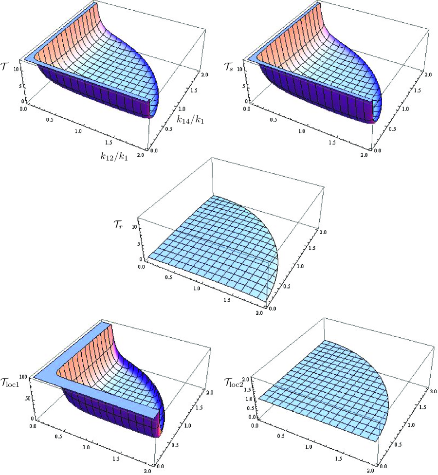
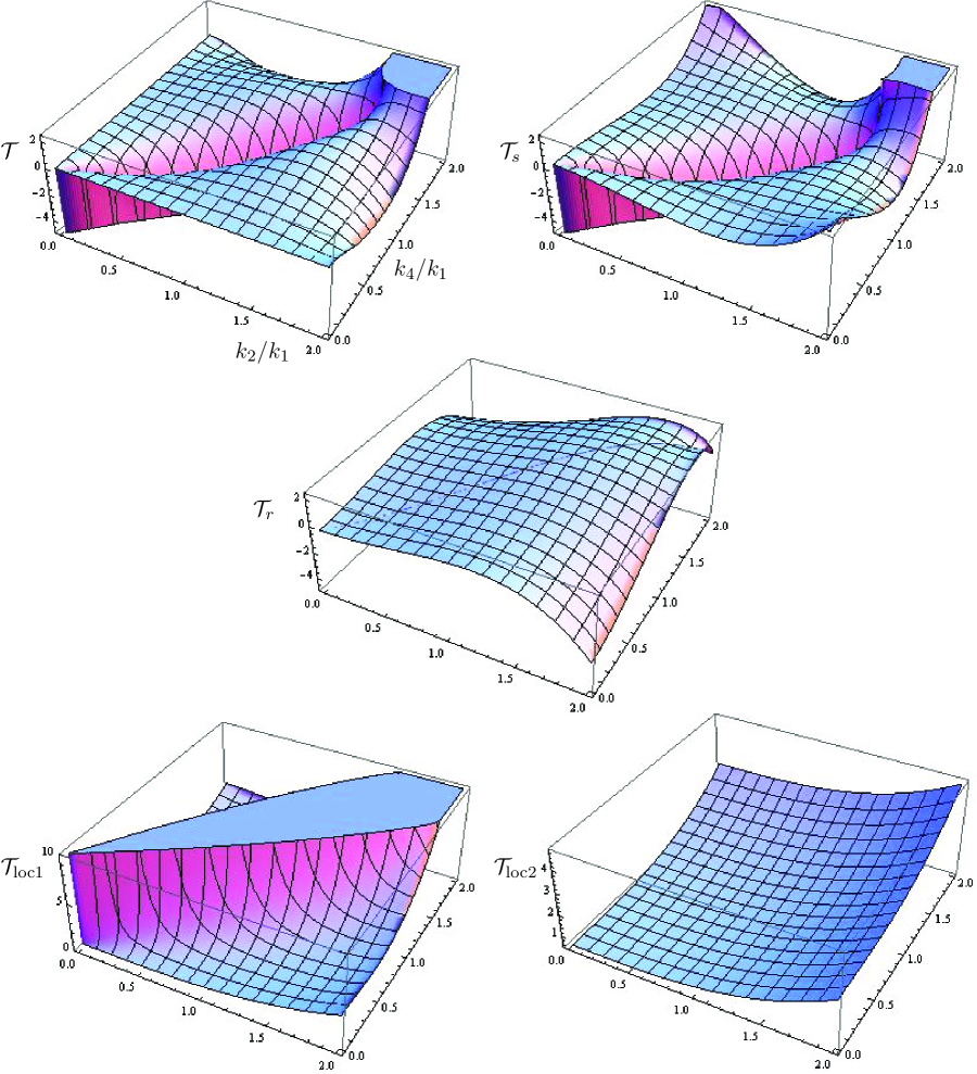
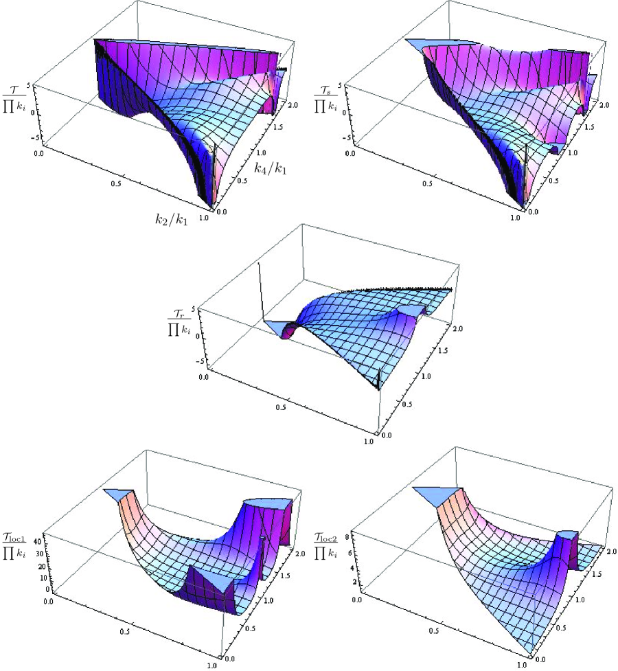
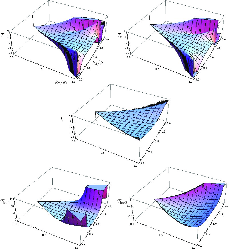
Let us consider various limits of the shape function $\mathcal{T}$. We use the nomenclature of Refs. [10, 15]. The first three panels in Figs. 1, 2, 3 and 4 show the complete trispectrum $\mathcal{T}$, the contribution of the singular part $\mathcal{T}_{s}$ and the regular part $\mathcal{T}_{r}$ in our model, respectively. The fourth and fifth panels show the two local trispectra $\mathcal{T}_{\mathrm{loc1}}$ and $\mathcal{T}_{\mathrm{loc2}}$. Note that vertical scales in the last two panels are different from each other and from vertical scales in the first three panels. The ranges of arguments in these figures are limited due to various inequalities obeyed by the momenta. In particular,

$$k_{12}^{2}+k_{14}^{2}\leq\sum\limits_{i=1}^{4}k_{i}^{2}\;,$$
$$\sqrt{k_{1}^{2}+k_{4}^{2}-2k_{1}k_{4}}\leq k_{14}\leq\sqrt{k_{1}^{2}+k_{4}^{2}+2k_{1}k_{4}}\;.$$

The limits we present are:

1. Equilateral limit, $k_{1}=k_{2}=k_{3}=k_{4}$. We plot in Fig. 1 the trispectra as functions of $k_{12}/k_{1}$ and $k_{14}/k_{1}$. Clearly seen is the singularity $\mathcal{T}\propto k_{12}^{-1},k_{14}^{-1}$ in our trispectrum and in its singular part, as well as stronger singularity $\mathcal{T}_{\mathrm{loc1}}\propto k_{12}^{-3},k_{14}^{-3}$ in the first local trispectrum. As we pointed out in Section 1, inflationary models produce trispectra without singularities at $k_{12}\to 0$ and/or $k_{14}\to 0$ [10, 12, 13, 14, 15]. Thus, the singularity, which is due to the infrared enhancement of the modes $\delta\rho$, is a distinctive feature of the conformal models.

2. Specialized planar limit, $k_{1}=k_{3}=k_{14}$ and

$$k_{12}=\left[k_{1}^{2}+\displaystyle\frac{k_{2}k_{4}}{2k_{1}^{2}}\left(k_{2}k_{4}+\displaystyle\sqrt{(4k_{1}^{2}-k_{2}^{2})(4k_{1}^{2}-k_{4}^{2})}\right)\right]^{1/2}\;.$$

The trispectra are shown in Fig. 2 as functions of $k_{2}/k_{1}$ and $k_{4}/k_{1}$. The structures along the diagonal are again due to the singularity, now at $k_{13}\to 0$, which corresponds to $k_{2}\to k_{4}$. Note that our total trispectrum vanishes at the boundaries $k_{2}=0$ and $k_{4}=0$ (this can be established analytically). The latter feature is similar to many inflationary models [10, 15], while it is absent for $\mathcal{T}_{\mathrm{loc1}}$ and $\mathcal{T}_{\mathrm{loc2}}$.

3. Near the double-squeezed limit, $k_{3}=k_{4}=k_{12}$. We show in Fig. 3 the combinations

$$\frac{\mathcal{T}}{\prod\limits_{i=1}^{4}k_{i}}\;,$$

and in Fig. 4 the trispectra $\mathcal{T}$ themselves as functions of $k_{2}/k_{1}$ and $k_{4}/k_{1}$. Clearly, our trispectrum is quite different from local ones in this limit.

4 Conclusions

By comparing the upper panels in Figs. 1, 2, 3, 4 one observes that the most notable features of the trispectrum in conformal models are well captured by its singular part, which has the factorized form (34). It is also clear that the trispectrum is substantially different from the trispectra of local forms. Furthermore, the comparison of our trispectrum with the trispectra given, e.g., in Refs. [10, 15] shows that our trispectrum is considerably different from the trispectra inherent in inflationary models. Hence, the shape of the non-Gaussianity, together with the statistical anisotropy, is an interesting signature of the conformal mechanisms.

As we observed in Section 2.2, models employing conformal invariance for generating the flat scalar power spectrum are indistinguishable at the leading non-linear order. It remains to be understood whether one can discriminate between concrete models from this class, even in principle. In any case, it would be extremely interesting to learn (or rule out) that, in a certain sense, our Universe started out conformal.

Note added. After this work has been published in arXive, the paper [24] appeared, where the results similar to those presented in Section 2 were obtained in much more general context. We are indebted to K. Hinterbichler and J. Khoury for making their paper available to us.

Acknowledgements

The authors are indebted to S. Ramazanov for useful comments and discussions. This work has been supported in part by the Federal Agency for Science and Innovations under state contract 02.740.11.0244 and by the grant of the President of the Russian Federation NS-5525.2010.2. The work of M.L. has been supported in part by RFBR grant 11-02-92108. The work of S.M. has been supported in part by RFBR grant 11-02-01220. M.L. and S.M. acknowledge the support by the Dynasty Foundation. The work of V.R. has been supported in part by the SCOPES program.

Refer to caption
Figure 1: Complete trispectrum $\mathcal{T}$ (upper left panel), its singular part $\mathcal{T}_{s}$ (upper right panel), its regular part $\mathcal{T}_{r}$ (middle panel), trispectrum of local form $\mathcal{T}_{\mathrm{loc1}}$ (lower left panel) and trispectrum of another local form $\mathcal{T}_{\mathrm{loc2}}$ (lower right panel) in equilateral limit. See Section 3.3 for definitions. Note that vertical scales in the lower panels are different, and neither coincides with the vertical scales in the three upper panels.
Refer to caption
Figure 2: Same as in Fig. 1, but in specialized planar limit.
Refer to caption
Figure 3: Near the double-squeezed limit. Shown are the combinations $\mathcal{T}/(\prod\limits_{i=1}^{4}k_{i})$ for the same trispectra as in Fig. 1.
Refer to caption
Figure 4: Near the double-squeezed limit. Same as in Fig. 3, but for the trispectra $\mathcal{T}$ themselves.

Appendix

In this Appendix we perform the complete calculation of the tripsectrum. Notably, this can be done analytically.

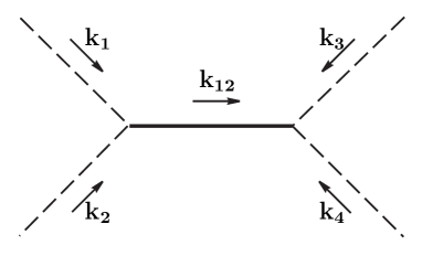
The computation is conveniently performed in terms of symmetric polynomials. For the $s$-channel diagram of Fig. 5 these are

$$K_{1}=k_{1}+k_{2}\;,\ \ K_{2}=k_{1}k_{2}\;,\ \ P_{1}=k_{3}+k_{4}\;,\ \ P_{2}=k_{3}k_{4}\;.$$
Refer to caption
Figure 5: $s$-channel diagram that contributes to the trispectrum. Dashed and solid lines correspond to the two-point functions of the fields $\theta$ and $\delta\rho$, respectively.

In what follows, we encounter the combinations

$$Z_{K_{1},K_{2}}=K_{1}(3K_{1}^{2}-12K_{2}-k_{12}^{2})\;,\ \ \ \ X_{K_{1},K_{2}}=k_{12}^{4}+2k_{12}^{2}(K_{1}^{2}-2K_{2})+12K_{1}^{2}K_{2}-3K_{1}^{4}\;.$$

In these notations, the expressions (28) and (29) read

$\displaystyle\tilde{R}$ $\displaystyle=$ $\displaystyle[K_{1}^{2}-2K_{2}-k_{12}^{2}-K_{2}(K_{1}^{2}-k_{12}^{2})\xi^{2}]\cos(K_{1}\xi)$
$\displaystyle+$ $\displaystyle K_{1}(K_{1}^{2}-2K_{2}-k_{12}^{2})\xi\sin(K_{1}\xi)\;,$
$\displaystyle\tilde{Q}$ $\displaystyle=$ $\displaystyle[K_{1}^{2}-2K_{2}-k_{12}^{2}-K_{2}(K_{1}^{2}-k_{12}^{2})\xi^{2}]\sin(K_{1}\xi)$
$\displaystyle-$ $\displaystyle K_{1}(K_{1}^{2}-2K_{2}-k_{12}^{2})\xi\cos(K_{1}\xi)\;.$

The terms (26) give the following contribution to the four-point function:

$$G_{4\ T\bar{T}}=\frac{h^{2}}{\prod\limits_{i=1}^{4}k_{i}^{3}}\frac{\pi}{32}\left[\phantom{\frac{\phantom{1}}{\phantom{1}}}\mathcal{U}(k_{1},k_{2},k_{3},k_{4},k_{12})+2~{}\mbox{permutations}\phantom{\frac{\phantom{1}}{\phantom{1}}}\right]\;,$$

where, in self-explaining notations,

$$\mathcal{U}(k_{1},k_{2},k_{3},k_{4},k_{12})=\frac{32}{\pi}\int\limits_{0}^{\infty}d\xi U(k_{1},k_{2},k_{3},k_{4},k_{12};\xi)$$

and

$\displaystyle U(k_{1},k_{2},k_{3},k_{4},k_{12};\xi)$ $\displaystyle=$ $\displaystyle\int\limits_{0}^{\xi}\frac{d\chi}{\sqrt{\xi\chi}}\left(J_{5/2}(k_{12}\xi)Y_{5/2}(k_{12}\chi)\phantom{\frac{\phantom{1}}{\phantom{1}}}\!\!\!-\!\!\!\phantom{\frac{\phantom{1}}{\phantom{1}}}Y_{5/2}(k_{12}\xi)J_{5/2}(k_{12}\chi)\right)$
$\displaystyle\times\left(\tilde{Q}_{k_{1},k_{2},k_{12}}(\xi)\tilde{R}_{k_{3},k_{4},k_{12}}(\chi)\phantom{\frac{\phantom{1}}{\phantom{1}}}\!\!\!+\!\!\!\phantom{\frac{\phantom{1}}{\phantom{1}}}\tilde{Q}_{k_{3},k_{4},k_{12}}(\xi)\tilde{R}_{k_{1},k_{2},k_{12}}(\chi)\right)\;.$

A tedious but straightforward calculation of the latter integral gives

$$U=U_{0}+U_{I}\;,$$

where

$\displaystyle U_{0}$ $\displaystyle=$ $\displaystyle\frac{\tilde{Q}_{k_{3},k_{4},k_{12}}(\xi)}{2\pi k_{12}^{5}\xi^{3}}\left(2k_{12}^{3}\xi\cos(K_{1}\xi)(2K_{2}k_{12}^{2}\xi^{2}-3(K_{1}^{2}-4K_{2}+k_{12}^{2}))\phantom{\frac{\phantom{1}}{\phantom{1}}}\right.$ (41)
$\displaystyle\left.\phantom{\frac{\phantom{1}}{\phantom{1}}}-2K_{1}k_{12}\sin(K_{1}\xi)(2k_{12}^{4}\xi^{2}+3k_{12}^{2}+36K_{2}-9K_{1}^{2})\right)+\{k_{1},k_{2}\leftrightarrow k_{3},k_{4}\},$
$\displaystyle U_{I}$ $\displaystyle=$ $\displaystyle\frac{\tilde{Q}_{k_{3},k_{4},k_{12}}(\xi)X_{K_{1},K_{2}}}{2\pi k_{12}^{5}\xi^{3}}\left(\left[(k_{12}^{2}\xi^{2}-3)\sin(k_{12}\xi)+3k_{12}\xi\cos(k_{12}\xi)\right]\phantom{\frac{\phantom{1}}{\phantom{1}}}\right.$
$\displaystyle\times\left.\left[\mathrm{Ci}((K_{1}-k_{12})\xi)+\mathrm{Ci}((K_{1}+k_{12})\xi)\right]\right.$
$\displaystyle+$ $\displaystyle\left.\left[(k_{12}^{2}\xi^{2}-3)\cos(k_{12}\xi)-3k_{12}\xi\sin(k_{12}\xi)\right]\right.$
$\displaystyle\left.\phantom{\frac{\phantom{1}}{\phantom{1}}}\times\left[\mathrm{Si}((K_{1}-k_{12})\xi)-\mathrm{Si}((K_{1}+k_{12})\xi)\right]\right)+\{k_{1},k_{2}\leftrightarrow k_{3},k_{4}\}\;.$

Note that $U_{0}$ contains only trigonometric functions and powers of $\xi$. So, the integration of $U_{0}$ over $\xi$ is cumbersome but straightforward555At $\xi\to 0$ the original integrals converge. Nevertheless, some particular terms may produce divergences (note, e.g., that $U_{0}$ contains $\cos(K_{1}\xi)/\xi$). To regularize these divergences we integrate over $\xi$ from $\alpha>0$ and take the limit $\alpha\to 0$ in the end of the calculation.. On the other hand, $U_{I}$ involves cosine and sine integrals Ci and Si, so the integration of it is tricky. We perform the latter integration by making use of the integral representations of the functions Si and Ci and changing the order of integration, i.e., we first integrate over $\xi$ and then integrate over $\chi$:

$\displaystyle\mathcal{U}_{I}$ $\displaystyle=\frac{32}{\pi}\int\limits_{0}^{\infty}d\xi U_{I}(\xi)$
$\displaystyle=\frac{32}{\pi^{2}}\int\limits_{0}^{\infty}\frac{\cos(K_{1}\chi)d\chi}{\chi}\int\limits_{0}^{\chi}d\xi\frac{\tilde{Q}_{k_{3},k_{4},k_{12}}(\xi)X_{K_{1},K_{2}}}{k_{12}^{5}\xi^{3}}$
$\displaystyle\times\left(\left[(3-k_{12}^{2}\xi^{2})\sin(k_{12}\xi)-3k_{12}\xi\cos(k_{12}\xi)\right]\cos(k_{12}\chi)\phantom{\frac{\phantom{1}}{\phantom{1}}}\right.$
$\displaystyle\left.\phantom{\frac{\phantom{1}}{\phantom{1}}}-\left[(3-k_{12}^{2}\xi^{2})\cos(k_{12}\xi)+3k_{12}\xi\sin(k_{12}\xi)\right]\sin(k_{12}\chi)\right)+\{k_{1},k_{2}\leftrightarrow k_{3},k_{4}\}$
$\displaystyle=\mathcal{U}_{I0}+\mathcal{U}_{II}.$

The inner integration over $\xi$ is lengthy but again straightforward. It again produces two types of contributions: the first one does not contain sine and cosine integrals,

$\displaystyle\mathcal{U}_{I0}$ $\displaystyle=\frac{16X_{K_{1},K_{2}}}{\pi^{2}k_{12}^{4}}\int\limits_{0}^{\infty}\frac{\cos(K_{1}\chi)d\chi}{\chi^{2}}\left(2P_{1}(k_{12}^{2}-3P_{2})\chi\cos(P_{1}\chi)+P_{1}(k_{12}^{2}+12P_{2}-3P_{1}^{2})\chi\cos(k_{12}\chi)\phantom{\frac{\phantom{1}}{\phantom{1}}}\right.$
$\displaystyle\left.\phantom{\frac{\phantom{1}}{\phantom{1}}}+[3P_{1}^{2}-6P_{2}-k_{12}^{2}(3-2P_{2}\chi^{2})]\sin(P_{1}\chi)\right)+\{k_{1},k_{2}\leftrightarrow k_{3},k_{4}\}\;,$ (42)

while the second one contains Si and Ci in the integrand,

$\displaystyle\mathcal{U}_{II}=\frac{8X_{K_{1},K_{2}}X_{P_{1},P_{2}}}{\pi^{2}k_{12}^{5}}\int\limits_{0}^{\infty}\frac{\cos(K_{1}\chi)d\chi}{\chi}\left(\cos(k_{12}\chi)\left[\mathrm{Ci}((P_{1}+k_{12})\chi)-\mathrm{Ci}((P_{1}-k_{12})\chi)\phantom{\frac{P1}{P1}}\right.\right.$
$\displaystyle-\left.\left.\log\left(\frac{P_{1}+k_{12}}{P_{1}-k_{12}}\right)\right]+\sin(k_{12}\chi)\left[\mathrm{Si}((P_{1}+k_{12})\chi)+\mathrm{Si}((P_{1}-k_{12})\chi)\right]\right)+\{k_{1},k_{2}\leftrightarrow k_{3},k_{4}\}\;.$ (43)

Nevertheless, both of these integrals can be evaluated analytically, the relevant formulas being

$\displaystyle S_{i}(a,b,c)$ $\displaystyle=$ $\displaystyle\lim_{\epsilon\to+0}\int\limits_{0}^{\infty}dx\mathrm{e}^{-\epsilon x}\frac{\sin(ax)\mathrm{Si}(bx)}{x}+\{b\rightarrow c\}$
$\displaystyle=$ $\displaystyle\frac{1}{4}\left[\Theta(b-a)L_{2}^{*}(b/a)+\Theta(a-b)L_{2}(b/a)-2L_{2}(-b/a)+L_{2}(b/a)\right]+\{b\rightarrow c\}\;,$
$\displaystyle C_{i}(a,b,c)$ $\displaystyle=\lim_{\epsilon\to+0}\int\limits_{0}^{\infty}dx\mathrm{e}^{-\epsilon x}\frac{\cos(ax)[\mathrm{Ci}(bx)-\mathrm{Ci}(cx)-\log(b/c)]}{x}$
$\displaystyle=\frac{1}{8}\left\{\log\left(\frac{b^{2}}{c^{2}}\right)\log\left(\frac{(ia)^{2}}{bc}\right)+L_{2}\left(\frac{b^{2}}{a^{2}}\right)-L_{2}\left(\frac{a^{2}}{b^{2}}\right)-L_{2}\left(\frac{c^{2}}{a^{2}}\right)+L_{2}\left(\frac{a^{2}}{c^{2}}\right)\right\}\;.$

where $L_{2}$ is the dilogarithm function. In this way we obtain

$\displaystyle\mathcal{U}$ $\displaystyle=\frac{1}{8\pi k_{12}^{4}}\left(Z_{k_{1},k_{2}}X_{k_{3},k_{4}}\log\left[\frac{(P_{1}^{2}-k_{12}^{2})^{2}}{(K_{1}+P_{1})^{4}}\right]+Z_{k_{3},k_{4}}X_{k_{1},k_{2}}\log\left[\frac{(K_{1}^{2}-k_{12}^{2})^{2}}{(K_{1}+P_{1})^{4}}\right]\right.$
$\displaystyle+\left.\frac{k_{12}^{2}}{(K_{1}+P_{1})^{3}}[{\cal G}_{2}+k_{12}^{2}{\cal G}_{4}+k_{12}^{4}{\cal G}_{6}]\right)$
$\displaystyle+\frac{1}{8\pi k_{12}^{5}}X_{k_{1},k_{2}}X_{k_{3},k_{4}}\left[C_{i}(K_{1}+k_{12},P_{1}+k_{12},P_{1}-k_{12})+C_{i}(K_{1}-k_{12},P_{1}+k_{12},P_{1}-k_{12})\phantom{\frac{\phantom{1}}{\phantom{1}}}\right.$
$\displaystyle+\left.S_{i}(K_{1}+k_{12},P_{1}+k_{12},P_{1}-k_{12})-S_{i}(K_{1}-k_{12},P_{1}+k_{12},P_{1}-k_{12})+\{k_{1},k_{2}\leftrightarrow k_{3},k_{4}\}\!\!\!\phantom{\frac{\phantom{1}}{\phantom{1}}}\right]\;.$

The first two lines here come from the integration of $U_{0}$, Eq. (41), and from (42), while the rest is due to (43). The notations are

$\displaystyle{\cal G}_{2}(k_{1},k_{2},k_{3},k_{4})$ $\displaystyle=$ $\displaystyle-12(K_{1}+P_{1})^{4}(K_{1}^{2}-4K_{2})(P_{1}^{2}-4P_{2})\;,$
$\displaystyle{\cal G}_{4}(k_{1},k_{2},k_{3},k_{4})$ $\displaystyle=$ $\displaystyle 32K_{2}P_{2}(K_{1}^{2}+K_{1}P_{1}+P_{1}^{2})$
$\displaystyle-$ $\displaystyle 16P_{2}(K_{1}+P_{1})(K_{1}^{3}+2K_{1}^{2}P_{1}-3K_{1}P_{1}^{2}-3P_{1}^{3})$
$\displaystyle-$ $\displaystyle 16K_{2}(K_{1}+P_{1})(P_{1}^{3}+2P_{1}^{2}K_{1}-3P_{1}K_{1}^{2}-3K_{1}^{3})$
$\displaystyle-$ $\displaystyle 4(K_{1}+P_{1})^{2}(3K_{1}^{4}-2K_{1}^{2}P_{1}^{2}+3P_{1}^{4})\;,$
$\displaystyle{\cal G}_{6}(k_{1},k_{2},k_{3},k_{4})$ $\displaystyle=$ $\displaystyle-32K_{2}P_{2}-16(K_{1}+P_{1})\left[K_{2}(K_{1}+2P_{1})+P_{2}(P_{1}+2K_{1})\right]$
$\displaystyle+$ $\displaystyle 4(K_{1}+P_{1})^{2}(3K_{1}^{2}+2K_{1}P_{1}+3P_{1}^{2})\;.$

We add the part of (25) that corresponds to the $s$-channel diagram of Fig. 5 and is given by (30), and obtain the overall contribution of the $s$-channel diagram:

$\displaystyle S(k_{1},k_{2},k_{3},k_{4},k_{12})$ $\displaystyle=$ $\displaystyle\frac{h^{2}}{\prod\limits_{i=1}^{4}k_{i}^{3}}\frac{\pi}{32}\left[\mathcal{Y}(k_{1},k_{2},k_{12})\mathcal{Y}(k_{3},k_{4},k_{12})+\mathcal{J}(k_{1},k_{2},k_{12})\mathcal{J}(k_{3},k_{4},k_{12})\phantom{\frac{\phantom{1}}{\phantom{1}}}\right.$ (44)
$\displaystyle\left.\phantom{\frac{\phantom{1}}{\phantom{1}}}+\mathcal{U}(k_{1},k_{2},k_{3},k_{4},k_{12})\right]\;.$

Together with crossing terms this yields our final result

$\displaystyle G_{4}(\mathbf{k}_{1},\mathbf{k}_{2},\mathbf{k}_{3},\mathbf{k}_{4})$ $\displaystyle=$ $\displaystyle\frac{h^{2}}{\prod\limits_{i=1}^{4}k_{i}^{3}}\mathcal{T}(k_{1},k_{2},k_{3},k_{4},k_{12},k_{14})=S(k_{1},k_{2},k_{3},k_{4},k_{12})$ (45)
$\displaystyle+S(k_{1},k_{3},k_{2},k_{4},k_{13})+S(k_{1},k_{4},k_{3},k_{2},k_{14}).$

References

  • [1] V. F. Mukhanov and G. V. Chibisov, JETP Lett.  33 (1981), 532; [Pisma Zh. Eksp. Teor. Fiz.  33 (1981), 549];
    S. W. Hawking, Phys. Lett.  B 115 (1982), 295;
    A. A. Starobinsky, Phys. Lett.  B 117 (1982), 175;
    A. H. Guth and S. Y. Pi, Phys. Rev. Lett.  49 (1982), 1110;
    J. M. Bardeen, P. J. Steinhardt and M. S. Turner, Phys. Rev.  D 28 (1983), 679.
  • [2] I. Antoniadis, P. O. Mazur and E. Mottola, Phys. Rev. Lett.  79 (1997) 14 [astro-ph/9611208].
  • [3] V. A. Rubakov, JCAP 0909 (2009), 030 [arXiv:0906.3693].
  • [4] P. Creminelli, A. Nicolis and E. Trincherini, JCAP 1011 (2010) 021 [arXiv:1007.0027].
  • [5] M. Osipov and V. Rubakov, JETP Lett.  93 (2011) 52 [arXiv:1007.3417].
  • [6] A. D. Linde and V. F. Mukhanov, Phys. Rev.  D 56 (1997), 535 [astro-ph/9610219];
    K. Enqvist and M. S. Sloth, Nucl. Phys.  B 626 (2002), 395 [hep-ph/0109214];
    D. H. Lyth and D. Wands, Phys. Lett.  B 524 (2002), 5 [hep-ph/0110002];
    T. Moroi and T. Takahashi, Phys. Lett.  B 522 (2001), 215 [Erratum-ibid.  B 539 (2002), 303] [hep-ph/0110096];
    K. Dimopoulos, D. H. Lyth, A. Notari and A. Riotto, JHEP 0307, (2003), 053 [hep-ph/0304050].
  • [7] G. Dvali, A. Gruzinov and M. Zaldarriaga, Phys. Rev.  D 69 (2004), 023505 [astro-ph/0303591];
    L. Kofman, astro-ph/0303614;
    G. Dvali, A. Gruzinov and M. Zaldarriaga, Phys. Rev.  D 69 (2004), 083505 [astro-ph/0305548].
  • [8] M. Libanov, S. Ramazanov and V. Rubakov, JCAP 1106, 010 (2011) [arXiv:1102.1390 [hep-th]].
  • [9] M. Libanov and V. Rubakov, JCAP 1011 (2010) 045 [arXiv:1007.4949].
  • [10] X. Chen, B. Hu, M. x. Huang, G. Shiu and Y. Wang, JCAP 0908 (2009) 008 [arXiv:0905.3494].
  • [11] M. Libanov, S. Mironov and V. Rubakov, arXiv:1012.5737.
  • [12] D. Seery, J. E. Lidsey and M. S. Sloth, JCAP 0701 (2007) 027 [astro-ph/0610210];
    X. Chen, M. x. Huang and G. Shiu, Phys. Rev.  D 74 (2006) 121301 [hep-th/0610235];
    D. Seery and J. E. Lidsey, JCAP 0701 (2007) 008 [astro-ph/0611034];
    F. Arroja and K. Koyama, Phys. Rev.  D 77 (2008) 083517 [arXiv:0802.1167];
    C. T. Byrnes, K. Y. Choi and L. M. H. Hall, JCAP 0902 (2009) 017 [arXiv:0812.0807];
    X. Gao, M. Li and C. Lin, JCAP 0911 (2009) 007 [arXiv:0906.1345];
    D. Langlois and L. Sorbo, JCAP 0908 (2009) 014 [arXiv:0906.1813];
    K. Izumi, T. Kobayashi and S. Mukohyama, JCAP 1010 (2010) 031 [arXiv:1008.1406];
    X. Gao and C. Lin, JCAP 1011 (2010) 035 [arXiv:1009.1311];
    L. Senatore and M. Zaldarriaga, arXiv:1009.2093;
    S. Mizuno and K. Koyama, JCAP 1010 (2010) 002 [arXiv:1007.1462];
    P. Creminelli, G. D’Amico, M. Musso, J. Norena and E. Trincherini, JCAP 1102 (2011) 006 [arXiv:1011.3004].
  • [13] D. Seery, M. S. Sloth and F. Vernizzi, JCAP 0903 (2009) 018 [arXiv:0811.3934].
  • [14] F. Arroja, S. Mizuno, K. Koyama and T. Tanaka, Phys. Rev.  D 80 (2009) 043527 [arXiv:0905.3641].
  • [15] N. Bartolo, M. Fasiello, S. Matarrese and A. Riotto, JCAP 1009 (2010) 035 [arXiv:1006.5411].
  • [16] D. H. Lyth, C. Ungarelli and D. Wands, Phys. Rev.  D 67 (2003) 023503 [arXiv:astro-ph/0208055];
    N. Bartolo, S. Matarrese and A. Riotto, Phys. Rev.  D 69 (2004) 043503 [arXiv:hep-ph/0309033];
    D. H. Lyth and Y. Rodriguez, Phys. Rev. Lett.  95 (2005) 121302 [arXiv:astro-ph/0504045];
    M. Sasaki, J. Valiviita and D. Wands, Phys. Rev.  D 74 (2006) 103003 [arXiv:astro-ph/0607627].
  • [17] M. Zaldarriaga, Phys. Rev.  D 69 (2004) 043508 [arXiv:astro-ph/0306006];
    T. Suyama and M. Yamaguchi, Phys. Rev.  D 77 (2008) 023505 [arXiv:0709.2545 [astro-ph]].
  • [18] K. Ichikawa, T. Suyama, T. Takahashi and M. Yamaguchi, Phys. Rev.  D 78 (2008) 063545 [arXiv:0807.3988 [astro-ph]].
  • [19] C. T. Byrnes and K. Y. Choi, Adv. Astron.  2010 (2010) 724525 [arXiv:1002.3110 [astro-ph.CO]].
  • [20] T. Okamoto and W. Hu, Phys. Rev.  D 66 (2002) 063008 [astro-ph/0206155].
  • [21] N. Kogo and E. Komatsu, Phys. Rev.  D 73 (2006) 083007 [astro-ph/0602099].
  • [22] A. Nicolis, R. Rattazzi and E. Trincherini, Phys. Rev.  D 79 (2009) 064036 [arXiv:0811.2197].
  • [23] J. M. Maldacena, JHEP 0305 (2003) 013 [astro-ph/0210603];
    S. Weinberg, Phys. Rev.  D 72 (2005), 043514 [hep-th/0506236].
  • [24] K. Hinterbichler and J. Khoury, arXiv:1106.1428 [hep-th].