IITM/PH/TH/2011/5 arXiv:1105.6231
v2.0

On the asymptotics of higher-dimensional partitions

Srivatsan Balakrishnan, Suresh Govindarajan and Naveen S. Prabhakar

Department of Physics, Indian Institute of Technology Madras,
Chennai 600036, India

We conjecture that the asymptotic behavior of the numbers of solid (three-dimensional) partitions is identical to the asymptotics of the three-dimensional MacMahon numbers. Evidence is provided by an exact enumeration of solid partitions of all integers $\leq 68$ whose numbers are reproduced with surprising accuracy using the asymptotic formula (with one free parameter) and better accuracy on increasing the number of free parameters. We also conjecture that similar behavior holds for higher-dimensional partitions and provide some preliminary evidence for four and five-dimensional partitions.

The purpose of computation is insight, not numbers. – Richard Hamming

1 Introduction

Partitions of integers appear in large number of areas such number theory, combinatorics, statistical physics and string theory. Several properties of partitions, in particular, its asymptotics (the Hardy-Ramanujan-Rademacher formula) can be derived due to its connection with the Dedekind eta function which is a modular form[1, 2]. In 1916, MacMahon introduced higher-dimensional partitions as a natural generalization of the usual partitions of integers[3]. He also conjectured generating functions for these partitions and was able to prove that his generating function for plane (two-dimensional) partitions was the correct one. However it turned out that his generating function for dimensions greater than two turned out to be incorrect. Even for plane partitions, one no longer has nice modular properties for the generating function. Nevertheless, the existence of a generating function enables one to derive asymptotic formulae for the numbers of plane partitions[4]. The inability to do the same with higher-dimensional partitions (for dimensions $>2$) has meant that these objects have not been studied extensively. The last detailed study, to the best of our knowledge, is due to Atkin et. al.[5].

Higher-dimensional partitions do appear in several areas of physics (as well as mathematics) and thus it is indeed of interest to understand them better. It is known that the infinite state Potts model in $(d+1)$ dimensions gets related to $d$-dimensional partitions[6, 7]. They also appear in the study of directed compact lattice animals[8]; in the counting of BPS states in string theory and supersymmetric field theory[9, 10]. For instance, it is known that the numbers of mesonic and baryonic gauge invariant operators in some $\mathcal{N}=1$ supersymmetric field theories get mapped to higher-dimensional partitions[9]. The Gopakumar-Vafa (Donaldson-Thomas) invariants (in particular, the zero-brane contributions) are also related to deformed versions of higher-dimensional partitions (usually plane partitions)[11, 12](see also [13]).

In this paper, we address the issue of asymptotics of higher-dimensional partitions as well as explicit enumeration of higher-dimensional partitions. Our work builds on the seminal work of Mustonen and Rajesh on the asymptotics of solid partitions[14]. lack of a simple formula for the generating functions of these partitions has been a significant hurdle in their study. The conjectures on the asymptotics of higher dimensional partitions given in this paper, even if partly true, would constitute progress in the study of higher-dimensional partitions. The conjecture on the asymptotics was arrived upon serendipitously by us when we found that a one-parameter formula for solid-partitions derived using MacMahon’s generating function worked a lot better than it should. To be precise, a formula that was meant to obtain an order of magnitude estimate (for solid partitions of integers in the range $[50,62]$) was not only getting the right order of magnitude but was also correct to $0.1-0.5\%$ (around 3-4 digits). The main conjecture discussed in section 3 is a natural outgrowth of this observation. The exact enumeration of solid partitions was possible due to an observation that lead to a gain of the order of $10^{4}$ to $10^{5}$ enabling us to exactly generate numbers of the order of $10^{16}-10^{17}$ in reasonable time.

The paper is organized as follows. Following the introductory section, section 2 provides the background to problem of interest as well as fixes the notation. Section 3 deals with asymptotics of higher-dimensional partitions. This done by means of two conjectures. We provide some evidence towards these conjectures with a fairly detailed study of solid partitions using a combination of exact enumeration as well as fits to the data. Section 4 provides the theoretical background to the method used for the exact enumeration of higher-dimensional partitions. We conclude in section 5 with some remarks on extensions of this work. In appendices A we work out the asymptotics of MacMahon numbers. Appendix B provides an ‘exact’ asymptotic formula for three-dimensional MacMahon numbers. In appendix C we present several tables that includes our results from exact enumeration as well some details of the fits for solid partitions.

2 Background

A partition of an integer $n$, is a weakly decreasing sequence $(a_{0},a_{1},a_{2},\ldots)$ such that

• $\sum_{i}a_{i}=n$ and

• $a_{i+1}\leq a_{i}\quad\forall\ i$.

For instance, $(2,1,1)$ is a partition of $4$. Define $p_{1}(n)$ to be the number of partitions of $n$. For instance,

$$4=3+1=2+2=2+1+1=1+1+1+1\quad\implies\quad p_{1}(4)=5\ .$$ (2.1)

A slightly more formal way definition of a partition is as a map from $\mathbb{Z}_{\geq 0}$ to $\mathbb{Z}_{\geq 0}$ satisfying the two conditions mentioned above. This definition enables one to generalise to higher dimensional partitions. A $d$-dimensional partition of $n$ is defined to be a map from $\mathbb{Z}_{\geq 0}^{d}$ to $\mathbb{Z}_{\geq 0}$ such that it is weakly decreasing along all directions and the sum of all its entries add to $n$. Let us denote the partition by $(a_{i_{1},i_{2},\ldots,i_{d}})$. The weakly decreasing condition along the $r$-th direction implies that

$$a_{i_{1},i_{2},\ldots,i_{r}+1,\ldots,i_{d}}\leq a_{i_{1},i_{2},\ldots,i_{r},\ldots i_{d}}\quad\forall\ (i_{1},i_{2},\ldots,i_{d})\ .$$ (2.2)

Two-dimensional partitions are also called plane partitions while three-dimensional partitions are also called solid partitions. Plane partitions can thus be written out as a two-dimensional array of numbers, $a_{ij}$. For instance, the two-dimensional partitions of $4$ are

$$\begin{smallmatrix}4\end{smallmatrix}\quad\begin{smallmatrix}3&1\end{smallmatrix}\quad\begin{smallmatrix}3\\ 1\end{smallmatrix}\quad\begin{smallmatrix}2&2\end{smallmatrix}\quad\begin{smallmatrix}2\\ 2\end{smallmatrix}\quad\begin{smallmatrix}2&1&1\end{smallmatrix}\quad\begin{smallmatrix}2&1\\ 1\end{smallmatrix}\quad\begin{smallmatrix}2\\ 1\\ 1\end{smallmatrix}\quad\begin{smallmatrix}1&1&1&1\end{smallmatrix}\quad\begin{smallmatrix}1&1&1\\ 1\end{smallmatrix}\quad\begin{smallmatrix}1&1\\ 1&1\end{smallmatrix}\quad\begin{smallmatrix}1&1\\ 1\\ 1\end{smallmatrix}\quad\begin{smallmatrix}1\\ 1\\ 1\\ 1\end{smallmatrix}\quad$$ (2.3)

Thus we see that there are $13$ two-dimensional partitions of $4$. Let us denote by $p_{d}(n)$ the number of $d$-dimensional partitions of $n$. It is useful to define the generating function of these partitions by ($p_{d}(0)\equiv 1$)

$$P_{d}(q)\equiv\sum_{n=0}^{\infty}p_{d}(n)\ q^{n}\ .$$ (2.4)

The generating functions of one and two-dimensional partitions have very nice product representations. One has the Euler formula for the generating function of partitions

$$P_{1}(q)=\frac{1}{\prod_{n=1}^{\infty}(1-q^{n})}\ ,$$ (2.5)

and the MacMahon formula for the generating function of plane partitions

$$P_{2}(q)=\frac{1}{\prod_{n=1}^{\infty}(1-q^{n})^{n}}\ .$$ (2.6)

MacMahon also guessed a product formula for the generating functions for $d>2$ that turned out to be wrong[5]. His guess is of the form

$$M_{d}(q)=\frac{1}{\prod_{n=1}^{\infty}(1-q^{n})^{\binom{n+d-2}{d-1}}}:=\sum_{n=0}^{\infty}m_{d}(n)\ q^{n}\ .$$ (2.7)

We will refer to the numbers $m_{d}(n)$ as the $d$-dimensional MacMahon numbers. It is easy to see that $M_{1}(q)=P_{1}(q)$ and $M_{2}(q)=P_{2}(q)$. However $M_{d}(q)\neq P_{d}(q)$ for $d>2$. An explicit formula (given by Atkin et. al.[5] or the book by Andrews[15]) for the number of $d$-dimensional partitions of $6$ is

$$p_{d}(6)=1+10d+27\binom{d}{2}+28\binom{d}{3}+11\binom{d}{4}+\binom{d}{5}\ .$$ (2.8)

Then, one can show that

$$m_{d}(6)-p_{d}(6)=\binom{d}{3}+\binom{d}{4}\ ,$$ (2.9)

which is non-vanishing for $d\geq 3$. Thus the MacMahon generating function fails to generate numbers of partitions when $d\geq 3$.

2.1 Presentations of higher-dimensional partitions

There are several ways to depict higher dimensional partitions. Recall that there is a one to one correspondence between (one-dimensional) partitions of $n$ and Ferrers (or Young) diagrams. The partition of $4$ corresponding to $3+1$ corresponds to the Ferrers diagram

$$\leavevmode{}\hbox{\raise 0.79999pt\hbox{\raise 8.09998pt\hbox{\lower 16.19995pt\hbox{\hbox{$\vtop{\offinterlineskip\openup-0.4pt\halign{&\ytableau@startbox{\ytableau@defarg}{}#\ytableau@endbox\cr\framebox{\vbox to8.09998pt{\vss\hbox to8.09998pt{\hss$\scriptstyle$\hss}\vss}}&\framebox{\vbox to8.09998pt{\vss\hbox to8.09998pt{\hss$\scriptstyle$\hss}\vss}}&\framebox{\vbox to8.09998pt{\vss\hbox to8.09998pt{\hss$\scriptstyle$\hss}\vss}}\cr\framebox{\vbox to8.09998pt{\vss\hbox to8.09998pt{\hss$\scriptstyle$\hss}\vss}}\cr}}$}}}}}\ .$$

Similarly, the plane partition $\begin{smallmatrix}3\\ 1\end{smallmatrix}$ can be represented by a Young tableau (i.e., a Ferrers diagram with numbers in the boxes) or as a ‘pile of cubes’ stacked in three dimensions (one of the corners of the cubes being located at $(0,0,0)$, $(0,0,1)$, $(0,0,2)$ and $(1,0,0)$ in a suitably chosen coordinate system)

$3$ $1$     

Similarly, $d$-dimensional partitions can be represented as a pile of hypercubes in $(d+1)$ dimensions.

We refer the reader to the work by Stanley (and references therein) for an introduction to plane partitions[16, 17]. The book by Andrews[15] provides a nice introduction to higher-dimensional partitions. Further the lectures by Wilf on integer partitions[18] and the notes by Finch on partitions[19] are also good starting points to existing literature on the subject.

3 Asymptotics of higher-dimensional partitions

In this section, we will discuss the asymptotics of higher-dimensional partitions. The absence of an explicit formula for the generating function for $d>2$ implies that there is no simple way to obtain the asymptotics of such partitions. In this regard, an important result due to Bhatia et. al. states that[8]

$$\lim_{n\rightarrow\infty}n^{-d/d+1}\log p_{d}(n)=\textrm{$d$-dependent constant.}$$ (3.1)

Conjecture 3.1

The constant in the above formula is identical to the one for the corresponding MacMahon numbers.

$$\lim_{n\rightarrow\infty}n^{-\frac{d}{d+1}}\log p_{d}(n)=\lim_{n\rightarrow\infty}n^{-\frac{d}{d+1}}\log m_{d}(n)=\frac{d+1}{d}\Big{[}d\ \zeta(d+1)\Big{]}^{\frac{1}{d+1}}=:\beta_{1}^{(d)}\ .$$ (3.2)

For three-dimensional partitions, this becomes a conjecture of Mustonen and Rajesh. Mustonen and Rajesh used Monte-Carlo simulations to compute the constant and showed that it is $1.79\pm 0.01$[14]. This is compatible with the conjecture since $\beta_{1}^{(3)}\sim 1.78982$.

It is important to know the sub-leading behavior of the asymptotics of higher-dimensional partitions in order to have quantitative estimate of errors. This is something we will provide in the next subsection. Before discussing the asymptotic behavior of the higher-dimensional partitions, it is useful to know the asymptotic behavior of the MacMahon numbers. A calculation shown in appendix A gives their sub-leading behavior. One obtains

$$\log m_{d}(n)\sim\sum_{r=1}^{d}\ \beta^{(d)}_{r}\ n^{\frac{d-r+1}{d+1}}+\gamma^{(d)}\log n+\delta^{(d)}\ .$$ (3.3)

The constants $\beta^{(d)}_{r}$ and $\gamma^{(d)}$ have been computed for $d=3,4,5$ in appendix A.

3.1 Towards a stronger conjecture

The number of $d$-dimensional partitions of $n$ can be obtained from the generating function $P_{d}(q)$ by inverting Eq. (2.4)

$$p_{d}(n)=\frac{1}{2\pi}\int_{-\pi}^{\pi}P_{d}(e^{iy})\ e^{-iny}\ dy\ .$$ (3.4)

Suppose we knew all the singularities of the function $P_{d}(q)$. The integral can be then be evaluated (at large $n$), for instance, by the saddle point method and adding up the contribution of all singularities thus obtaining an asymptotic formula for $p_{d}(n)$. The singularities are usually obtained by looking at product formulae of the form

$$P_{d}(q)=\prod_{n=1}^{\infty}(1-q^{n})^{-a^{(d)}(n)}\ .$$ (3.5)

The exponents $a^{(d)}(n)$ can be determined for those values of $n$ for which $p_{d}(n)$ has been determined. If all the $a^{(d)}(n)$ are positive, then it is easy to see that $P_{d}(q)$ is singular at all roots of unity – this leads naturally to the circle method of Hardy and Ramanujan[1]. However, for $d>2$, this turns out to be false. For instance, $a^{(3)}(15)=-186$ is the first exponent that becomes negative for $d=3$[20, see Table 1]. We will assume that the singularities of $P_{d}(q)$ continues to occur at roots of unity. In particular, we will see that the Bhatia et. al. result implies that for large enough $n$, one has

$$a^{(d)}(n)=\mathcal{O}(n^{d-1})\ ,$$ (3.6)

with $a^{(d)}(n)>0$. Let us assume that the dominant term in a saddle point computation of the integral in Eq. (3.4) occurs near $q=1$.

Proposition 3.2

The Laurent expansion of $\log P_{d}(e^{-t})$ in the neighbourhood of $t=0$ is of the form

$$-\log P_{d}(e^{-t})=\frac{\widehat{C}_{d}}{d\,t^{d}}+\frac{\widehat{C}_{d-1}}{(d-1)\,t^{d-1}}+\cdots+\frac{\widehat{C}_{1}}{t}+\textrm{non-singular as }t\rightarrow 0\ ,$$ (3.7)

where $\widehat{C}_{1},\ldots,\widehat{C}_{d}$ are some constants.

Remark: This is precisely the form of the Laurent expansion for $\log M_{d}(e^{-t})$ near $t=0$ (see Appendix A).

A saddle point computation of the integral (3.4) is carried out by extremizing the function

$$\log P_{d}(e^{-t})+nt\ .$$

The extremum, $t_{*}$, which is close to $t=0$ for large $n$, obtained using Proposition 3.2 is given by

$$t_{*}=\left(\frac{\widehat{C}_{d}}{n}\right)^{1/(d+1)}+\cdots$$ (3.8)

Plugging in the saddle point value, we see that

$$\log p_{d}(n) \sim\frac{\widehat{C}_{d}}{d\,t_{*}^{d}}+\frac{\widehat{C}_{d-1}}{(d-1)\,t_{*}^{d-1}}+\cdots+\frac{\widehat{C}_{1}}{t_{*}}+nt_{*}+\cdots$$ (3.9)

$$\sim\frac{d+1}{d}\left(\widehat{C}_{d}\right)^{1/(d+1)}n^{d/(d+1)}+\textrm{sub-leading terms}\ .$$ (3.10)

We thus recover the bound obtained by Bhatia et. al.[8]. Thus, we see that the Bhatia et. al. result combined with the assumption that $P_{d}(e^{-t})$ is a meromorphic function in the neighborhood of $t=0$ with a pole of order $d$ implies Proposition 3.2.

A more precise saddle point computation enables us to determine sub-leading terms as well and we obtain

$$\log p_{d}(n)\sim\sum_{r=1}^{d}\ \widehat{\beta}^{(d)}_{r}\ n^{\frac{d-r+1}{d+1}}+\widehat{\gamma}^{(d)}\log n+\widehat{\delta}^{(d)}+\cdots\ ,$$ (3.11)

where the constants $\widehat{\beta}^{(d)}_{r}$, $\widehat{\gamma}^{(d)}$ and $\widehat{\delta}^{(d)}$ are determined by the constants $\widehat{C}_{r}$ that appear in Proposition 3.2.

Conjecture 3.1 implies that $\widehat{C}_{d}=d\,\zeta(d+1)$ – this is the leading coefficient in the Laurent expansion of $\log M_{d}(e^{-t})$ near $t=0$. This is equivalent to

$$a^{(d)}(n)=\frac{n^{d-1}}{(d-1)!}+\cdots\ ,$$ (3.12)

where the ellipsis indicates sub-leading terms in the large $n$ limit. We now propose a stronger form of conjecture 3.1.

Conjecture 3.3

The asymptotics of the $d$-dimensional partitions are identical to the asymptotics of the MacMahon numbers.

$$\log p_{d}(n)\sim\sum_{r=1}^{d}\ \beta^{(d)}_{r}\ n^{\frac{d-r+1}{d+1}}+\gamma^{(d)}\log n+\cdots\ ,$$ (3.13)

where $\beta^{(d)}_{r}$ and $\gamma^{(d)}$ are as in Eq. (3.3).

It is easy to see that one can have conjectures that are stronger than conjecture 3.1 but weaker than conjecture 3.3 by requiring fewer coefficients to match with Eq. (3.3). Conjecture 3.3 implies that the coefficients, $\widehat{C}_{r}$ ($r=1,\ldots,d$) in the Laurent expansion in Proposition 3.2 are identical to those of $\log M_{d}(e^{-t})$. Equivalently,

$$P_{d}(e^{-t})-M_{d}(e^{-t})=\mathcal{O}(1)\ ,$$ (3.14)

near $t=0$. It also implies that at large $n$, $a^{(d)}(n)$ behaves exactly like the exponent that appears in the product formula for $d$-dimensional MacMahon numbers in Eq. (2.7), i.e.,

$$a^{(d)}(n)\sim\binom{n+d-2}{d-1}+\cdots\ ,$$ (3.15)

where the ellipsis indicates terms that vanish as $n\rightarrow\infty$.

3.2 Evidence for the conjecture

We will provide evidence by explicitly enumerating numbers for the higher-dimensional partitions. In particular, we compute all solid partitions for $n\leq 68$ and use the formula provided by Eq. (3.13) as a one-parameter function to fit known numbers. The advantage of this procedure is that one doesn’t need to go to enormously large values of $n$. In Figures 1, 2 and 3, we compare this formula implied by conjecture 3.3 for $d=3,4,5$ respectively. Since the values of $n$ that we consider are not too large, these fits provide weak evidence that three of the conjectured numbers i.e., $\beta^{(d)}_{1}$, $\beta^{(d)}_{2}$ and $\gamma^{(d)}$ are probably correct.

$N$	$q_{3}(N)$	$p_{3}(N)$
58	3972318521718539	3971409682633930
59	6522014363273781	6520649543912193
60	10686367929548727	10684614225715559
61	17474590403967699	17472947006257293
62	used to fit constant	28518691093388854
63	46453074905306481	46458506464748807
64	75522726337662733	75542021868032878
65	122556018966297693	122606799866017598
66	198518226269824763	198635761249922839
67	320988410810838956	321241075686259326
68	518102330350099210	518619444932991189

Table 1: Estimates using the asymptotic formula $q_{3}(N)$. The constant in the asymptotic formula is fixed by requiring it to give the exact answer for $N=62$ – the largest known number of solid partitions at the time of the fit.

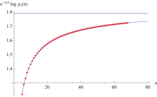
Figure 1: Plot of $n^{-3/4}\log p_{3}(n)$ for $n\in[5,68]$ (red dots). The blue curve is the asymptotic formula normalized to give the correct answer for $n=62$ and the horizontal line is the conjectured value for $n\rightarrow\infty$.

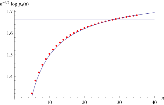
Figure 2: Plot of $n^{-4/5}\log p_{4}(n)$ for $n\in[5,35]$ (red dots). The blue curve is the asymptotic formula normalized to give the correct answer for $n=30$ and the horizontal line is the conjectured value for $n\rightarrow\infty$.

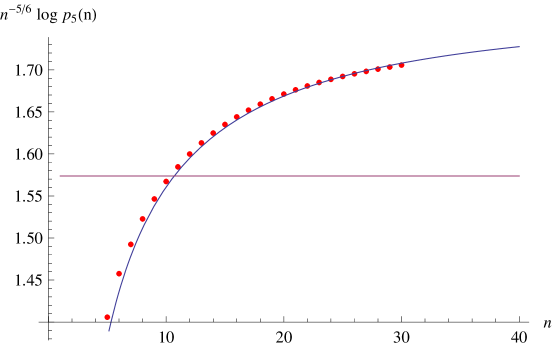
Figure 3: Plot of $n^{-5/6}\log p_{5}(n)$ for $n\in[5,30]$ (red dots). The blue curve is the asymptotic formula normalized to give the correct answer for $n=25$ and the horizontal line is the conjectured value for $n\rightarrow\infty$.

3.3 Solid partitions: a detailed study

The asymptotic expansion of the logarithm of three-dimensional MacMahon numbers is (with $\xi\equiv n+\tfrac{\zeta(-3)}{4}$)

$$\log m_{3}(n)\sim\frac{4}{3}[3\zeta(4)]^{1/4}\ \xi^{3/4}+\frac{\zeta(3)}{2[3\zeta(4)]^{1/2}}\ \xi^{1/2}-\frac{\zeta(3))^{2}}{8[3\zeta(4)]^{5/4}}\ \xi^{1/4}-\frac{61}{96}\log\xi+\cdots$$ (3.16)

Using the above formula as a guide, we fit the solid partitions to the following three formulae involving up to three parameters $(a,b,c)$: ($\xi:=n+b$)

$$q_{3}(n) =\frac{4}{3}[3\zeta(4)]^{1/4}\ n^{3/4}+\frac{\zeta(3)}{2[3\zeta(4)]^{1/2}}\ n^{1/2}-\frac{\zeta(3))^{2}}{8[3\zeta(4)]^{5/4}}\ n^{1/4}-\frac{61}{96}\log n+a$$

$$r_{3}(n) =\frac{4}{3}[3\zeta(4)]^{1/4}\ \xi^{3/4}+\frac{\zeta(3)}{2[3\zeta(4)]^{1/2}}\ \xi^{1/2}-\frac{\zeta(3))^{2}}{8[3\zeta(4)]^{5/4}}\ \xi^{1/4}-\frac{61}{96}\log\xi+a$$

$$s_{3}(n) =\frac{4}{3}[3\zeta(4)]^{1/4}\ \xi^{3/4}+\frac{\zeta(3)}{2[3\zeta(4)]^{1/2}}\ \xi^{1/2}-c\ \xi^{1/4}-\frac{61}{96}\log\xi+a\ .$$

Note that the number of free parameters increases from $1$ for the function $q_{3}$ to $2$ for $r_{3}$ and to $3$ for $s_{3}$. We obtain $a=-1.544$, $(a,b)=(-1.530,-0.028)$ and $(a,b,c)=(-3.211,1.689,0.257)$ from the three fits. We use the same functions to estimate the values of three-dimensional MacMahon numbers for the same range of values using a similar fit. We see that the function $s_{3}$ has worked almost as well as it did for the corresponding MacMahon numbers. In particular, the fit gives $c=0.25713$ which is different from the one given by MacMahon numbers for $\beta^{(3)}_{3}=-0.041413$. For the MacMahon numbers, the fitted value of $c=-0.057621$ which is close to the actual number. This suggests that the coefficient of $n^{1/4}$ may be different from the one given by the MacMahon numbers. For the values of $n$ that we have considered, the dominant contributions are due to the first two terms as well as the log term. Hence, we consider this as possible evidence for $\widehat{\beta}^{(3)}_{r}=\beta^{(3)}_{r}$ for $r=1,2$. For completeness, we provide the numbers obtained by carrying out a five-parameter fit using the numbers in the range $[60,68]$. The fit gives:

$$\log p_{3}(n)\sim 1.73\ n^{3/4}+0.83\ n^{1/2}-0.90\ n^{1/4}-1.00\ \log n-0.22\ .$$ (3.17)

We also observe that if we used a larger range of numbers, say, $n\in[50,68]$, we obtain large numbers (of order ten or greater) for some of the coefficients. This reflects the lack of data for large number more than anything else.

In an attempt at understanding the accuracy of our numbers better, we carried out a systematic study of an exact asymptotic formula (in the sense of Hardy-Ramanujan-Rademacher for partitions) for three-dimensional MacMahon numbers using a method due to Almkvist[21, 22]. These are discussed in Appendix B. One writes

$$m_{3}(n)\sim\sum_{k=1}^{\infty}\phi_{k}(n)\ ,$$

where $\phi_{k}(n)$ are the contributions from various saddle-points with $k=1$ being the dominant one. For $n=60$, we see that $\phi_{1}(60)$ gets the first nine digits right while the sum of the first two terms get eleven digits right. We further broke up the contribution of $\phi_{1}(n)$ into several terms. The term that we write as $\phi_{1}^{(0)}(n)$ is the contribution from the singular part of $\log M_{3}(e^{-}t)$ at the dominant saddle point located near $t=0$. We see that $\phi_{1}^{(0)}(60)$ gets the first five digits right – somewhat closer to what we have obtained in our estimates for the numbers of solid partitions.

3.4 An unbiased estimate for the leading coeffficient

In order to provide an unbiased estimate for the leading coefficient of the asymptotic formula using the exact numbers of solid partitions, we use the method of Neville tables (albeit with a slight and obvious modification)[23]. Let

$$e_{n}^{0} \equiv n^{-3/4}\log p_{3}(n)$$

$$\sim\sum_{x=1}^{3}\hat{\beta}_{x}^{(3)}n^{(1-r)/4}+\hat{\gamma}^{(3)}n^{-3/4}\log n+\hat{\delta}^{(3)}n^{-3/4}\ ,$$ (3.18)

where we have written the asymptotic formula in the second line using the parameters defined in Eq. (3.11). Further, for $r\geq 1$, recursively define

$$e_{n}^{r}:=\frac{n^{1/4}\ e_{n}^{r-1}-(n-r)^{1/4}\ e_{n-1}^{r-1}}{n^{1/4}-(n-r)^{1/4}}\ .$$ (3.19)

Using the conjectured asymptotic formula for $p_{3}(n)$, we can derive asymptotic formulae for $e_{n}^{r}$. The $e_{n}^{r}$ have been constructed so that

1. $\lim_{n\rightarrow\infty}e_{n}^{r}$ tends to a constant that equals $\hat{\beta}^{(3)}_{1}$ for all $r$. The first sub-leading term is proportional to $n^{-(r+1)/4}$. Thus a plot of $e_{n}^{r}$ vs $n^{-(r+1)/4}$ should be a straight line in the asymptotic limit.

2. As we increase $r$, the number of parameters that appear in the asymptotic formula for $e_{n}^{r}$ decrease. For instance, one sees that $\hat{\beta}_{2}^{(3)}$ drops out for $r=1$:

   $$e_{n}^{1}\sim\hat{\beta}^{(3)}_{1}-\hat{\beta}_{3}^{(3)}n^{-1/2}-2\hat{\gamma}^{(3)}n^{-3/4}\log n+(4\hat{\gamma}^{(3)}-2\hat{\delta}^{(3)})n^{-3/4}\ ,$$ (3.20)

   and $\hat{\beta}_{2}^{(3)},\ \hat{\beta}_{3}^{(3)}$ drop out for $r=2$:

   $$e_{n}^{2}\sim\hat{\beta}^{(3)}_{1}+\hat{\gamma}^{(3)}n^{-3/4}\log n+(-6\hat{\gamma}^{(3)}+\hat{\delta}^{(3)})n^{-3/4}\ ,$$ (3.21)

An estimate for $\hat{\beta}^{(3)}_{1}$ has been obtained by carrying out two and three-parameter fits to the asymptotic formula given in Eq. (3.20). We obtain

$$e_{n}^{1}=\left\{\begin{matrix}1.793+2.099n^{-1/2}&\textrm{two-parameter fit}\\ 1.781+0.83n^{-1/2}+0.924\log n&\textrm{three-parameter fit}\end{matrix}\right.$$ (3.22)

A four-parameter fit leads to coefficients that are not of order one. We discard this fit as we make the natural assumption that all coefficients are of order one or smaller. Using the two different fits, we can estimate $\hat{\beta}^{(3)}_{1}$ is around $1.78-1.79$. The wide variation that we observe in $\hat{\beta}^{(3)}_{2}$ suggests that we cannot estimate it with the available exact numbers. In figure 4, we have plotted $e_{n}^{1}$ vs $n^{-1/2}$ along with the three-parameter fit. We also observe that $e_{n}^{2}$ (see figure 5) is oscillating between $[1.77,1.81]$ and hence we cannot estimate any further parameters using the data. For completness, we have carried out a similar analysis for the MacMahon numbers, $m_{3}(n)$ in the range $n\in[20,68]$ and obtain $\beta^{(3)}_{1}$ in the range $[1.77-1.78]$. We also observe that $e_{n}^{2}$ does not oscillate as it does for solid partitions.

We conclude that an unbiased estimate for $\hat{\beta}^{(3)}$ is consistent with conjecture 3.1. However, given the relatively small values of $n$ that we have used, this only constitutes weak evidence at best. There is another result due to Widom et. al. who studied the asymptotics of (restricted) solid partitions with Ferrers diagrams that fit in a four-dimensional box of size $10^{3}\times p$[24] as a function of $p$. They observe that the entropy in the thermodynamic limit deviates from a formula derived from a MacMahon formula for restricted solid partitions. Should we expect a similar behavior for unrestricted solid partitions? The deviation observed by Widom et. al. is small. If a similar behavior occurs for unrestricted partitions, then conjecture 3.1 would be false. We believe that the exact numbers that we have used are not large enough to definitively test conjecture 3.1. However, in any case, it is important to note that that the functional form of the asympotics continues to hold.

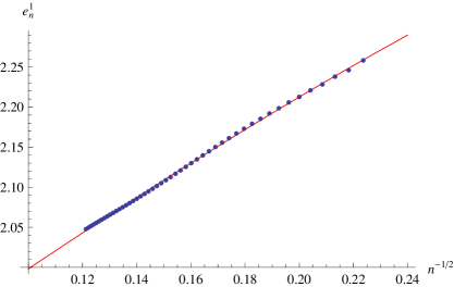
Figure 4: A plot of $e_{n}^{1}$ vs $n^{-1/2}$ for $n\in[20,68]$ along with a three-parameter fit.

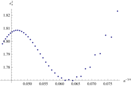
Figure 5: A plot of $e_{n}^{2}$ vs $n^{-3/4}$ for $n\in[20,68]$.

4 Explicit Enumeration

In this section, we discuss the explicit enumeration of higher dimensional partitions. The first program to explicitly enumerate higher-dimensional partitions is due to Bratley and McKay[25]. However, we do not use their algorithm but another one due to Knuth[20]. We start with a few mathematical preliminaries in order to understand the Knuth algorithm as well as our parallelization of the algorithm.

4.1 Almost Topological Sequences

Let $P$ be a set with a partial ordering (given by a relation denoted by $\prec$) and a well-ordering (given by a relation denoted by $<$). Further, let the partial ordering be embedded in the well-ordering i..e, $x\prec y$ implies $x<y$.

Definition 4.1

A sequence $\mathbf{X}=(x_{1},x_{2},\ldots,x_{m})$ containing elements of $P$ is called a topological sequence if[20]

1. For $1\leq j\leq m$ and $x\in P$, $x\prec x_{j}$ implies $x=x_{i}$ for some $i<j$;

2. If $m>0$, there exists $x\in P$ such that $x<x_{m}$ and $x\neq x_{i}$, for $1<i\leq m$.

Let us call a $j$-th position in a topological sequence, $\mathbf{X}$, interesting if $x_{j}>x_{j+1}$. By definition, the last position of a sequence is considered interesting. The index of a topological sequence is defined to be the sum of all $j$ for all interesting positions i.e.,

$$\textrm{index}(\mathbf{X})=\sum_{j}\left\{j~{}|~{}j\textrm{ is interesting}\right\}\ .$$ (4.1)

Definition 4.2

An almost topological sequence is a sequence that satisfies condition 1 but not necessarily condition 2.

Thus all topological sequences are also almost topological sequences. This definition is motivated by the observation that almost topological sequences do occur as sub-sequences of topological sequences.

4.1.1 An example due to Knuth

Let $P$ denote the set of three-dimensional lattice points i.e.,

$$P=\Big{\{}(i,j,k)~{}|~{}i,j,k=0,1,2,3,\ldots\Big{\}}\equiv\mathbb{N}^{3}$$ (4.2)

with the partial ordering $(i,j,k)\preceq(i^{\prime},j^{\prime},k^{\prime})$ if $i\leq i^{\prime}$, and $j\leq j^{\prime}$ and $k\leq k^{\prime}$. Let us choose the well-ordering to be given by the lexicographic ordering i.e.,

$$(i,j,k)<(i^{\prime},j^{\prime},k^{\prime})$$ (4.3)

if and only if

$$i<i^{\prime}\quad\textrm{ or }(i=i^{\prime}\textrm{ and }j<j^{\prime})\quad\textrm{ or }(i=i^{\prime},\ j=j^{\prime}\textrm{ and }k<k^{\prime})\ .$$

The depth of a topological sequence is the number of elements in the sequence. Consider the topological sequence (of depth $6$)

$$\mathbf{X}=\{(0,0,0),(0,0,1),(0,0,2),\mathbf{(1,0,0)},\mathbf{(0,1,0)},\mathbf{(0,0,3)}\}$$

where we have indicated the interesting positions in boldface. This sequence has index $15=4+5+6$.

4.2 Topological sequences and solid partitions

Let $d_{m}(n)$ denote the number of topological sequences of the set $P=\mathbb{N}^{m}$ with index $n$. Further, define $d_{m}(0)=1$. As before, let $p_{m}(n)$ denote the number of $m$-dimensional partitions of $n$. A theorem of Knuth relates these two sets of numbers as follows:

Theorem 4.3 (Knuth[20])

$$p_{m}(n)=\sum_{k=0}^{n}d_{m}(k)\ p_{1}(n-k)\ .$$ (4.4)

Equivalently, the generating function of $m$-dimensional partitions decomposes into a product of the generating function of the numbers of topological sequences and the generating function of one-dimensional partitions.

$$P_{m}(q)=D_{m}(q)\ P_{1}(q)\ ,$$ (4.5)

where

$$D_{m}(q):=\sum_{n=0}^{\infty}d_{m}(n)\ q^{n}\ .$$

Since topological sequences are much easier to enumerate, Knuth went ahead and wrote a program to generate all topological sequences of index $\leq N$ (for some fixed $N$). This is the program that was the starting point of our exact enumeration.

We list below the topological sequences of index 2 and 3 when $P=\mathbb{N}^{3}$ (we have dropped the comma between numbers to reduce the length of the expression)

Index 2: $$\ \big{\{}(000)(010)\big{\}}\quad\textrm{and}\quad\big{\{}(000)(100)\big{\}}\quad\implies\boxed{d_{3}(2)=2}\ .$$

Index 3: $$\ \big{\{}(000)(001)(010)\big{\}}\ ;\big{\{}(000)(001)(100)\big{\}}\ ;\big{\{}(000)(010)(020)\big{\}}\ ;$$

$$\big{\{}(000)(010)(100)\big{\}}\ ;\big{\{}(000)(100)(200)\big{\}}\quad\implies\boxed{d_{3}(3)=5}\ .$$

Thus, we see that $D_{3}(q)=1+2q^{2}+5q^{3}+\cdots$. We also have $P_{1}(q)=1+q+2q^{2}+3q^{3}+\cdots$. Thus, we obtain

$$P_{3}(q)=D_{3}(q)\ g_{1}(q)=1+q+4q^{2}+10q^{3}+\cdots$$

4.3 Equivalence classes of almost topological sequences

We say that two sequences $\mathbf{X}=(x_{1},x_{2},\ldots,x_{m})\sim\mathbf{Y}=(y_{1},y_{2},\ldots,y_{m})$ are related if the elements of $\mathbf{Y}$ are a permutation of the elements of $\mathbf{X}$. Of course, not all permutations of an almost topological sequence lead to another almost topological sequence as some of them violate condition 1 in the definition of a topological sequence. However, even after imposing the restriction to permutations that lead to other topological sequences, the relation remains an equivalence relation. As an example consider the following three sequences in $\mathbb{N}^{3}$:

$$\big{\{}(0,0,0),(0,0,1),(0,0,2),(1,0,0)\big{\}}\ ,$$

$$\big{\{}(0,0,0),(0,0,1),(1,0,0),(0,0,2)\big{\}}\ ,$$ (4.6)

$$\big{\{}(0,0,0),(1,0,0),(0,0,1),(0,0,2)\big{\}}\ .$$

It is easy to see that these three sequences form a single equivalence class. However, the last two are not topological sequences as they violate condition 2 in the definition of a topological sequence. and hence are almost topological sequences. We thus choose to work with equivalence classes of almost topological sequences.

Proposition 4.4

The equivalence classes of almost topological sequences of $\mathbb{N}^{d}$ of depth $k$ is in one to one correspondence with $(d-1)$-dimensional partitions of $k$. We shall refer to the $(d-1)$-dimensional partition as the shape of the equivalence class.

The $(d-1)$-dimensional partition is obtained by placing $d$-dimensional hypercubes (of size one) at the points appearing the almost topological sequence. This is nothing but the ‘piles of cubes’ representation of a $(d-1)$-dimensional partition. In this representation, the precise ordering of the points in the almost topological sequence is lost and one obtains the same $(d-1)$-dimensional partition for any element in the same equivalence class. Given a $(d-1)$-dimensional partition, the coordinates of the hypercubes in the ‘piles of cubes’ representation give the elements of the almost topological sequence. For instance, the equivalence class in Eq. (4.3) has as its shape the following two-dimensional partition of $4$:

$$\leavevmode{}\raise 0.0pt\hbox{\hbox{$\vtop{\offinterlineskip\openup-0.4pt\halign{&\ytableau@startbox{\ytableau@defarg}{}#\ytableau@endbox\cr\framebox{\vbox to15.00002pt{\vss\hbox to15.00002pt{\hss$3$\hss}\vss}}\cr\framebox{\vbox to15.00002pt{\vss\hbox to15.00002pt{\hss$1$\hss}\vss}}\crcr}}$}}\hbox{\raise 0.79999pt\hbox{\raise 15.00002pt\hbox{\lower 0.0pt}}}\qquad\qquad\includegraphics[height=39.83385pt]{31.eps}\quad.$$

When $P=\mathbb{N}^{2}$, the almost topological sequences of $P$ are standard Young tableaux. Given an almost topological sequence of $\mathbb{N}^{2}$ with shape $\lambda$ with $n$ boxes, the standard Young tableau is obtained by entering the position of the box in the almost topological sequence. It is easy to see that this map is a bijection. It is an interesting and open problem to enumerate the number of almost topological sequences given a shape for higher-dimensions. We did this by generating all topological partitions of a given index and sorting them out by shape. However, this is an overkill if one is interested in enumerating topological sequences associated with a particular shape.

4.4 Programming Aspects

The explicit enumeration of topological sequences to generate partitions was first carried out Knuth who enumerated solid partitions of integers $\leq 28$[20]. This was extended to all integers $\leq 50$ by Mustonen and Rajesh (using other methods)[14]. We first ported Knuth’s Algol program to C++ and quickly found that it was prohibitively hard to generate additional numbers given the fact that $p_{3}(50)$ is of the order of $10^{13}$. So we decided to parallelize Knuth’s program in the following way.

1. Generate all almost topological sequences up to a depth $k$.

2. Next, separately run each sequence (to generate the rest of tree) from depth $(k+1)$ until all sequences of index $N$ that contain the initial sequence as its first $k$ terms are generated. Here it is important to note that while we are counting the numbers of topological sequences, we need to include all almost topological sequences since they necessarily appear as sub-sequences of topological sequences.

3. An important observation is that it suffices to run one sequence for every given shape since they have identical tree structure after the $(k+1)$-th node. However, it is crucial to note that each topological sequence in a given equivalence class does not have the same index. This entails a bit of book keeping where one keeps track of the different indices of all topological sequences of identical shape. The power of this approach is best illustrated by looking at Table 2 where we list the numbers of actual sequences (nodes) as well the number of shapes. A naive estimate (based on the reduction of the number of runs) shows that run times should go down by an order of $10^{5}-10^{6}$.

Depth	12	14	15	17
Nodes	28680717	1567344549	12345147705	856212871761
Shapes	1479	4167	6879	18334

Table 2: Number of equivalence classes at various depths (equal to the number of plane partitions) for counting topological partitions of $\mathbb{N}^{3}$.

This approach has enabled us to extend the Knuth-Mustonen-Rajesh results to all integers $N\leq 68$. The numbers were generated in several steps: $N=52,55,62,68$. The results for $N\leq 52$ we obtained without parallelization. The results for $N\leq 55$ were obtained using parallelization to depth $7$ but without using equivalence classes and required about 1500 hours of CPU time. The results for $N\leq 62$ were done using parallelization to depth $14$ ($4167$ shapes) and took around 30000 hours of CPU time(about a month of runtime). The last set of results for $N\leq 68$ took around $360K$ hours of runtime (spread over five months).

We also extended the numbers for four-dimensional partitions of $N\leq 35$ and five-dimensional partitions of $N\leq 30$. This was done without any parallelization. The complete results are given in appendix C.

5 Conclusion

We believe that our results show that it is indeed possible to understand the asymptotics of higher dimensional partitions. The preliminary nature of our results shows that a lot more can and should be done. Our results provide a functional form to which results from Monte Carlo simulations, of the kind carried out by Mustonen and Rajesh[14], can be fitted to. However, the errors should be better than one part in $10^{3}$ or $10^{4}$ to be able to fix the sub-leading coefficients. We are indeed making preliminary studies to see whether one can achieve this.

Another avenue is to see if there are sub-classes of partitions that can be counted i.e., we can provide simple expressions for their generating functions. For instance, the analog of conjugation in usual partitions is the permutation group, $S_{d+1}$, for $d$-dimensional partitions. Following Stanley[26], we can organise $d$-dimensional partitions based on the subgroups of $S_{d+1}$ under which they are invariant (see also [27]). Some of these partitions might have simple generating functions.

One of the proofs of the MacMahon formula for the generating function of plane partitions is due to Bender and Knuth[28](see also [29]). It is done by considering a bijection between plane partitions and matrices with non-negative entries. There is a natural generalization of such matrices into hypermatrices – these hypermatrices are counted by MacMahon numbers. It would be interesting to contruct a Bender-Knuth type map between solid partitions and hypermatrices and study how it fails to be a bijection. This might explain why the asymptotics of MacMahon numbers works so well for higher-dimensional partitions.

Acknowledgments: We would like to thank Arun Chaganty, Prakash Mohan, S. Sivaramakrishnan as well the other undergraduate students of IIT Madras’ Boltzmann group who provided a lot of inputs to the project on the exact enumeration of solid partitions (http://boltzmann.wikidot.com/solid-partitions). We thank the High Performance Computing Environment (http://hpce.iitm.ac.in) at IIT Madras for providing us with a stable platform (the leo and vega superclusters) that made the explicit enumeration of higher-dimensional partitions possible. We thank Nicolas Destainville for drawing our attention to ref. [24].

Appendix A Asymptotics of the MacMahon numbers

In this appendix, we work out the asymptotics of the MacMahon numbers using a method due to Meinardus[30]. A nice introduction to this method is found in the paper by Lucietti and Rangamani[10].

We have seen that the generating function for $d$-dimensional MacMahon numbers is given by

$$M_{d}(q)=1+\sum_{n=1}^{\infty}m_{d}(n)\,q^{n}=\prod_{n=1}^{\infty}\frac{1}{(1-q^{n})^{\binom{n+d-2}{d-1}}}\ .$$ (A.1)

Inverting this, we obtain:

$$m_{d}(n)=\oint_{\Gamma}\frac{dq}{2{\pi}i}\frac{M_{d}(q)}{q^{n+1}}$$ (A.2)

where $q$ is a complex variable and $\Gamma$ is a circle $|q|=\varepsilon<1$ traversed in the counterclockwise direction. We shall evaluate the contour integral in (A.2) by writing $q=e^{-t}$ and then taking the limit $t\to 0$. This corresponds to the contribution to (A.2) due to the pole at $q=1$, which is the dominant contribution. The poles of $M_{d}(q)$ occur precisely at all roots of unity, with the sub-dominant contributions coming from other roots of unity.

We have,

$$\log M_{d}(e^{-t})=-\sum_{n=1}^{\infty}a_{n}\log(1-e^{-tn}),\quad a_{n}=\binom{n+d-2}{d-1}.$$ (A.3)

We expand the logarithm inside the sum using its Taylor series and using the Mellin representation of $e^{-x}$ i.e.,

$$e^{-x}=\frac{1}{2{\pi}i}\int_{\gamma-i\infty}^{\gamma+i\infty}\,ds\,x^{-s}\,\Gamma(s)\ ,\quad\gamma>0\ .$$ (A.4)

We obtain

$$\log M_{d}(e^{-t})=\frac{1}{2{\pi}i}\int_{\gamma-i\infty}^{\gamma+i\infty}\,ds\,\Gamma(s)\,\zeta(s+1)\,D_{d}(s)\,{t}^{-s}\ ,$$ (A.5)

where the Dirichlet series $D_{d}(s)$ defined as

$$D_{d}(s)=\sum_{n=1}^{\infty}\,\frac{a_{n}}{n^{s}}\ .$$

The real constant $\gamma$ is chosen to lie to the right of all poles of $D_{d}(s)$ in the $s$-plane. For $d=3$, $a_{n}=n(n+1)/2$ and hence the Dirichlet series is

$$D_{3}(s)=\sum_{n=1}^{\infty}\,\frac{n(n+1)}{2\,n^{s}}=\tfrac{1}{2}\big{[}\zeta(s-2)+\zeta(s-1)\big{]}\ .$$

Hence, $D_{3}(s)$ has simple poles at $s=2,3$ with residue $1/2$ at both poles. For general $d$, $D_{d}(s)$ has poles at $s=k,\,k=2,3,\ldots,d$. Let us denote the residue at $s=k$ by $A_{k}$.

Now, we shift the contour in (A.5) from Re$(s)=\gamma$ to Re$(s)=-\alpha$, for $0<\alpha<1$. In the process, $\log M_{d}(q)$ receives contributions from the poles of the integrand that lie between Re$(s)=\gamma$ and Re$(s)=-\alpha$. Hence, we get

$$\log M_{d}(e^{-t})=\sum_{k=2}^{d}A_{k}\,\Gamma(k)\,\zeta(k+1){t}^{-k}+D_{d}^{\prime}(0)-D_{d}(0)\log{t}\\ +\frac{1}{2{\pi}i}\int_{-\alpha-i\infty}^{-\alpha+i\infty}ds\,\Gamma(s)\,\zeta(s+1)\,D_{d}(s)\,{t}^{-s}.$$ (A.6)

The integral can be shown to go as $\mathcal{O}(|t|^{\alpha})$. Hence, we get

$$M_{d}(e^{-t})=\exp\Big{(}\sum_{k=2}^{d}A_{k}\,\Gamma(k)\,\zeta(k+1)\,{t}^{-k}+D_{d}^{\prime}(0)-D_{d}(0)\log{t}\Big{)}\Big{(}1+\mathcal{O}(|t|^{\alpha})\Big{)}$$ (A.7)

Hence, near $q=1$, we have

$$m_{d}(n)=\frac{1}{2{\pi}i}\int_{t_{0}-i\pi}^{t_{0}+i\pi}dt\,e^{G_{d}(t)}.$$ (A.8)

where ($t_{0}$ is taken to close to $0^{+}$)

$$G_{d}(t)=\sum_{k=2}^{d}\frac{C_{k}}{k\,{t}^{k}}+nt\ ,\qquad C_{k}:=A_{k}\,\Gamma(k+1)\,\zeta(k+1)$$

We carry out the integral (A.8) using the saddle point method. For this, we have to first evaluate $t=t_{*}$ such that $G^{\prime}_{d}(t_{*})=0$. That is,

$$\sum_{k=2}^{d}\frac{C_{k}}{t_{*}^{k+1}}-n=0.$$ (A.9)

We next let the integration contour pass through the saddle point for which the value of $G_{d}(t_{*})$ is largest. This happens when $t_{*}$ is the largest root of (A.9). This means $t_{*}^{-(d+1)}\sim n$ or equivalently, $t_{*}\sim n^{-1/d+1}$ and hence, $t_{*}\to 0$ as $n\to\infty$. Hence, the saddle point method indeed gives the value of $m_{d}(n)$ for $n\to\infty$.

Now, we solve for $t_{*}$ from (A.9) which is a polynomial equation of degree $d+1$. For $d>3$, we do not have a general formula for the roots of the equation. But in this case, we indeed have a formula for the largest positive root of (A.9), due to Lagrange:

$$t_{*}(n)=\sum_{\begin{subarray}{c}\ell\,>\,0\\ \ell\neq 0\textrm{ mod }(d+1)\end{subarray}}^{\infty}b_{\ell}\,n^{-\ell/(d+1)}$$ (A.10)

where

$$b_{\ell}=\frac{1}{\ell!}\Bigg{[}\frac{d^{\ell-1}}{dy^{\ell-1}}\phi(y)^{\ell}\Bigg{]}_{y=0}\textrm{ with }\quad\phi(y)\equiv\Bigg{(}\sum_{k=1}^{d}C_{k}\,y^{d-k}\Bigg{)}^{\frac{1}{d+1}}.$$

Using the above formula, we can compute $t_{0}$ to any required order in $n$ and then carry out the saddle-point integration (A.9). We finally get

$$m_{d}(n)=\sqrt{\frac{1}{2{\pi}G_{d}^{\prime\prime}(t_{*})}}\ t_{*}^{-D_{d}(0)}\>\exp\big{(}G_{d}(t_{*})+D_{d}^{\prime}(0)\big{)}\,\Big{(}1+\mathcal{O}\left(t_{*}^{\alpha}\right)\Big{)}\ .$$ (A.11)

Recall that the dependence on $n$ occurs implicitly, on the right hand side of the above equation, through the saddle-point value $t_{*}(n)$.

A.1 Three-dimensional MacMahon numbers

The asymptotic formula is

$$m_{3}(n)\sim\textrm{const }n^{-61/96}\ \exp(\widehat{G}_{3}(n))\ ,$$ (A.12)

where

$$\widehat{G}_{3}(n):=\frac{4}{3}{C_{3}}^{1/4}n^{3/4}+\frac{C_{2}}{2C_{3}^{2/4}}\,n^{2/4}+\frac{\left(8C_{1}C_{3}-C_{2}^{2}\right)}{8C_{3}^{5/4}}\,n^{1/4}$$

with $C_{1}=0$, $C_{2}=\zeta(3)$ and $C_{3}=3\zeta(4)$. Numerically evaluating, we obtain

$$\widehat{G}_{3}(n)\simeq 1.78982n^{3/4}+0.333546\sqrt{n}-0.0414393n^{1/4}\ .$$ (A.13)

A.2 Four-dimensional MacMahon numbers

The asymptotic formula is

$$m_{4}(n)\sim\textrm{const }n^{-2179/3600}\ \exp(\widehat{G}_{4}(n))\ ,$$ (A.14)

where

$$\widehat{G}_{4}(n):=\frac{5}{4}{C_{4}}^{1/5}n^{4/5}+\frac{C_{3}n^{3/5}}{3C_{4}^{3/5}}+\frac{\left(5C_{2}C_{4}-C_{3}^{2}\right)}{10C_{4}^{7/5}}\,n^{2/5}+\frac{\left(C_{3}^{3}-5C_{2}C_{4}C_{3}+25C_{1}C_{4}^{2}\right)}{25C_{4}^{11/5}}\,n^{1/5}$$

with $C_{1}=0$, $C_{2}=2\zeta(3)/3$, $C_{3}=3\zeta(4)$ and $C_{4}=4\zeta(5)$. Numerically evaluating, we obtain

$$\widehat{G}_{4}(n)\simeq 1.66139\ n^{4/5}+0.460969\ n^{3/5}+0.0829315\ n^{2/5}-0.0345152\ n^{1/5}\ .$$ (A.15)

A.3 Five-dimensional MacMahon numbers

The asymptotic formula is

$$m_{5}(n)\sim\textrm{const }n^{-563/960}\ \exp(\widehat{G}_{5}(n))\ ,$$ (A.16)

where

$$\widehat{G}_{5}(n):= \frac{6}{5}C_{5}^{1/6}\,n^{5/6}+\frac{C_{4}}{4C_{5}^{2/3}}\,n^{4/6}+\frac{\left(4C_{3}C_{5}-C_{4}^{2}\right)}{12C_{5}^{3/2}}\,n^{3/6}$$

$$+\frac{\left(2C_{4}^{3}-9C_{3}C_{5}C_{4}+27C_{2}C_{5}^{2}\right)}{54C_{5}^{7/3}}\,n^{2/6}$$

$$+\frac{\left(-91C_{4}^{4}+504C_{3}C_{5}C_{4}^{2}-864C_{2}C_{5}^{2}C_{4}+432C_{5}^{2}\left(12C_{1}C_{5}-C_{3}^{2}\right)\right)}{5184C_{5}^{19/6}}\ n^{1/6}\ ,$$

with $C_{1}=0$, $C_{2}=\tfrac{1}{2}\zeta(3)/3$, $C_{3}=\tfrac{11}{4}\zeta(4)$, $C_{4}=6\zeta(5)$ and $C_{5}=5\zeta(6)$. Numerically evaluating, we obtain

$$\widehat{G}_{5}(n)=1.5737\ n^{5/6}+0.525874\ n^{2/3}+0.15873\ \sqrt{n}+0.0223817\ n^{1/3}-0.0263759\ n^{1/6}\ .$$ (A.17)

Appendix B A rather exact formula for $m_{3}(n)$

We will work out the asymptotics of the three-dimensional MacMahon numbers using methods due to Almkvist[21, 22]. The generating function of three-dimensional MacMahon numbers is

$$M_{3}(x)=\prod_{n=1}^{\infty}(1-x^{n})^{-n(n+1)/2}=\sum_{n=0}^{\infty}m_{3}(n)\ x^{n}\ .$$ (B.1)

The integrals are evaluated using the circle method due to Hardy and Ramanujan[1]. The coefficients $m_{3}(n)$ are determined from the generating function by the formula

$$m_{3}(n)=\frac{1}{2\pi}\int_{-\pi}^{\pi}M_{3}\big{(}e^{iy}\big{)}\ e^{-iny}dy\ .$$ (B.2)

Since $M_{3}(x)$ has poles when ever $x$ is a root of unity, the dominant contributions occur in the neighborhood of this point. Setting $x=\exp(iy)$, we see that the poles occur for all $y=2\pi h/k$ with $(h,k)=1$ the contribution can be evaluated by summing over contributions from such terms. One writes

$$m_{3}(n) \sim\sum_{k=1}^{\infty}\sum_{\begin{subarray}{c}h=1\\ (h,k)=1\end{subarray}}^{k-1}\frac{1}{2\pi}\int_{\gamma_{h,k}}M_{3}\big{(}e^{i(2\pi h/k+\varphi)}\big{)}\ e^{-in(2\pi h/k+\varphi)}d\varphi\ ,$$ (B.3)

$$\sim\sum_{k=1}^{\infty}\phi_{k}(n)$$ (B.4)

where $\gamma_{h,k}$ is an arc passing through $\varphi=0$. We don’t give a detailed discussion on the choice of the arc but refer the interested reader to [31]. In the second line, we have implicitly assumed that the integrals and the sum over $h$ have been carried out.

In order to carry out the integral for a particular $(h,k)$, we need to compute the Laurent expansion of $M_{3}(x)$ about the point $x=\exp(2\pi ih/k)$ and then compute the integral using methods such as the saddle point. For usual partitions, this is typically done using modular properties of the Dedekind eta function. However, there is no such modular property in this case. The dominant contribution occurs for $k=1$ (or $x=1$) and we will first consider this contribution. Let

$$g_{3d}(t):=\log M_{3}(e^{-t})=-\tfrac{1}{2}\sum_{\nu=1}^{\infty}\nu(\nu+1)\ \log(1-e^{-\nu t})\equiv\sum_{\nu=1}^{\infty}h_{3d}(\nu),$$ (B.5)

where $h_{3d}(x):=-\tfrac{x(x+1)}{2}\ \log(1-e^{-xt})$.The Abel-Plana formula enables us to replace the discrete sum over $\nu$ by the integral:

$$g_{3d}(t)=\int_{0}^{\infty}h(x)\ dx-i\int_{0}^{\infty}\frac{h(iy)-h(-iy)}{e^{2\pi y}-1}\ dy\ ,$$ (B.6)

For $h_{r}(x):=-x^{r}\log(1-e^{-xt})$ , by expanding out the logs and resumming, Almkvist has shown that[22]

$$g_{r}(t) =\Big{[}\tfrac{r!\zeta(r+2)}{t^{r+1}}+\zeta^{\prime}(-r)-\zeta(-r)\log t+\frac{t}{2}\zeta(-r-1)\Big{]}+\sum_{\nu=2}^{\infty}\tfrac{\zeta(1-\nu)\zeta(-r-\nu)}{\nu!}t^{\nu}\ ,$$

$$=\hat{g}_{r}(t)+g^{sum}_{r}(t)\ ,$$ (B.7)

where in the second line $g^{sum}_{r}(t)$ refers to terms appearing as the sum in the first line and $\hat{g}_{r}(t)$ the remaining terms (within square brackets) up to order $t$. This separation is useful in computing the saddle-point where we will drop the terms appearing in $g^{sum}_{r}(t)$ in computing the location of the saddle point. Then, it follows that

$$g_{3d}(t)=\frac{1}{2}\Big{(}g_{1}(t)+g_{2}(t)\Big{)}\quad\implies\quad\boxed{M_{3}(e^{-t})\sim\exp\big{[}\tfrac{g_{1}(t)+g_{2}(t)}{2}\big{]}}\ .$$ (B.8)

Note that the infinite sum for $g_{2}(t)$ vanishes since $\zeta(-2n)=0$ for $n=1,2,3,\ldots$ while for $g_{1}(t)$ only terms with even $\nu$ contribute. In computing the integral in Eq. (B.3), we

$$\frac{1}{2\pi}\int_{\gamma_{1,1}}M_{3}\left(e^{i\varphi}\right)\ d\varphi=\frac{e^{\tfrac{1}{2}[\zeta^{\prime}(-1)+\zeta^{\prime}(-2)]}}{2\pi}\int_{-\infty}^{\infty}(-i\varphi)^{-\hat{\gamma}}e^{\left(\tfrac{a_{1}}{2(-i\varphi)^{2}}+\tfrac{2a_{2}}{2(-i\varphi)^{3}}-i\xi\varphi\right)}\ d\varphi$$ (B.9)

where $a_{1}=\zeta(3)$, $a_{2}=2\zeta(4)$, $\hat{\gamma}=\zeta(-1)/2=-1/24$ and $\xi=n+\tfrac{\zeta(-3)}{4}$. Using the expansion

$$\exp\left(\tfrac{a_{1}}{2(-i\varphi)^{2}}+\tfrac{2a_{2}}{2(-i\varphi)^{3}}\right)=\sum_{\nu_{1},\nu_{2}}\frac{a_{1}^{\nu_{1}}a_{2}^{\nu_{2}}}{2^{\nu_{1}+\nu_{2}}\nu_{1}!\nu_{2}!(-i\varphi)^{2\nu_{1}+3\nu_{2}}}$$ (B.10)

and the integral

$$\frac{1}{2\pi}\int_{-\infty}^{\infty}(-i\varphi)^{-\alpha}e^{-i\xi\varphi}\ d\varphi=\left\{\begin{array}[]{ll}\frac{\xi^{\alpha-1}}{\Gamma(\alpha)}&\textrm{ if }\alpha\geq 1\\ \delta(\xi)&\textrm{ if }\alpha=0\end{array}\right.$$ (B.11)

we find that the contribution ignoring the terms in $g^{sum}_{3d}(t)$ is given by

$$\phi^{(0)}_{1}(n) \sim\exp\big{(}\tfrac{1}{2}[\zeta^{\prime}(-1)+\zeta^{\prime}(-2)]\big{)}\sum_{(\nu_{1},\nu_{2})\in\mathbb{N}^{2}}\frac{a_{1}^{\nu_{1}}a_{2}^{\nu_{2}}}{2^{\nu_{1}+\nu_{2}}\nu_{1}!\nu_{2}!}\frac{\xi^{2\nu_{1}+3\nu_{2}-1+\hat{\gamma}}}{\Gamma(2\nu_{1}+3\nu_{2}+\hat{\gamma})}$$

$$:=\exp\big{(}\tfrac{1}{2}[\zeta^{\prime}(-1)+\zeta^{\prime}(-2)]\big{)}\ L[\xi,\hat{\gamma}]\ ,$$ (B.12)

where we have implicitly defined the function $L[\xi,\gamma]$ in the second line. In order to include the contribution of $g^{sum}_{3d}(t)$, we consider the Taylor expansion (Note that $c_{0}=1$)

$$\exp\Big{(}g^{sum}_{3d}(t)\Big{)}=\sum_{j=0}^{\infty}c_{j}\ t^{j}\ ,$$ (B.13)

and carry out the integrations to obtain

$$\phi_{1}(n) =\sum_{j=0}^{\infty}\phi^{(j)}_{1}(n)$$

$$:=\exp\big{(}\tfrac{1}{2}[\zeta^{\prime}(-1)+\zeta^{\prime}(-2)]\big{)}\sum_{j=0}^{\infty}c_{j}\ L\left[n+\tfrac{\zeta(-3)}{4},\hat{\gamma}-j\right]$$ (B.14)

B.1 Other poles

Let us evaluate $M_{3d}\big{(}e^{iy}\big{)}$ in the neighbourhood of such a point. Put $y=2\pi h/k+\varphi$ and using a method due to Almkvist(see Theorem 5.1 in [22]), we get

$$M_{3d}\big{(}e^{i2\pi h/k-i\varphi}\big{)}\sim\exp\Big{(}\tfrac{1}{2}\left[\tfrac{a_{1}}{k^{3}}(-i\varphi)^{-2}+\tfrac{a_{2}}{k^{4}}(-i\varphi)^{-3}\right]+\tfrac{1}{2}\big{[}k\zeta^{\prime}(-1)+k^{2}\zeta^{\prime}(-2)\big{]}\\ +\tfrac{\pi i}{2}\big{[}s(1,h,k)+s(2,h,k)\big{]}-\frac{k}{2}\zeta(-1)\log(-ik\varphi)-\tfrac{1}{4}\zeta(-3)i\varphi+\cdots\Big{)}\ ,$$ (B.15)

where the generalized Dedekind sums are

$$s(1,h,k) =\frac{k}{3}\sum_{j=1}^{k-1}B_{2}(j/k)\log|2\sin(jh\pi/k)|+\frac{ik^{2}t}{8}\sum_{j=1}^{k-1}B_{3}(j/k)\cot(jh\pi/k)$$

$$s(2,h,k) =\frac{k}{3}\sum_{j=1}^{k-1}B_{3}(j/k)((jh/k))=-\frac{1}{16k}\sum_{j=1}^{k-1}\cot^{(r)}(jh\pi/k)\cot(j\pi/k)\ ,$$ (B.16)

where $B_{n}(x)$ are the Bernoulli polynomials and

$$((x))=\left\{\begin{array}[]{lr}x-[x]-\tfrac{1}{2}&\textrm{ if }x\notin\mathbb{Z}\\ 0&\textrm{ if }x\in\mathbb{Z}\end{array}\right.$$ (B.17)

We illustrate the computation of $\phi_{1}(n)$ for $n=60$. Below, we quote the result after rounding off to the nearest integer and underline the number of correct digits.

$$\phi_{1}^{(0)}(60) =\underline{11031}748252850258$$

$$\phi^{(0)}_{1}(60)+\phi^{(1)}_{1}(60) =\underline{1103128}7052778130$$

$$\phi_{1}(60) =\underline{110312866}33959406$$

$$\phi_{1}(60)+\phi_{2}(60) =\underline{11031286641}929870$$

$$m_{3}(60) =11031286641714044$$

We observe that $\phi_{1}^{(0)}(60)$ gets the first five digits right while $\phi_{1}(60)$ makes the estimate correct to nine digits while adding $\phi_{2}(60)$ gets 11 digits right. We need to include the contributions of of other zeros i.e., $\phi_{k}(n)$ for $k>2$ to further improve the estimate. We anticipate that addition of other terms should eventually lead to an exact answer though we have not explicitly verified that it is so.

Appendix C Exact enumeration of higher-dim. partitions

In this appendix, we provide the results obtained from our exact enumeration of three, four and five-dimensional partitions. In all cases, we have gone significantly beyond what is known and we have contributed our results to the Online Encyclopedia of Integer Sequences(OEIS) – the precise sequence is listed in the table. We believe that it will be significantly harder to add to the numbers of solid partitions as the generation of the last set of numbers took around five months. In this case, adding a single number roughly doubles the runtime. There is, however, some scope for improvement for the four and five-dimensional partitions as the numbers were generated without parallelization.

$$\begin{array}[]{|rr|rr|rr|}\hline\cr n&p_{3}(n)&n&p_{3}(n)&n&p_{3}(n)\\[2.0pt] \hline\cr 0&1&23&19295226&46&8683676638832\\ 1&1&24&35713454&47&14665233966068\\ 2&4&25&65715094&48&24700752691832\\ 3&10&26&120256653&49&41495176877972\\ 4&26&27&218893580&50&69531305679518\\ 5&59&28&396418699&51&116221415325837\\ 6&140&29&714399381&52&193794476658112\\ 7&307&30&1281403841&53&322382365507746\\ 8&684&31&2287986987&54&535056771014674\\ 9&1464&32&4067428375&55&886033384475166\\ 10&3122&33&7200210523&56&1464009339299229\\ 11&6500&34&12693890803&57&2413804282801444\\ 12&13426&35&22290727268&58&3971409682633930\\ 13&27248&36&38993410516&59&6520649543912193\\ 14&54804&37&67959010130&60&10684614225715559\\ 15&108802&38&118016656268&61&17472947006257293\\ 16&214071&39&204233654229&62&28518691093388854\\ 17&416849&40&352245710866&63&46458506464748807\\ 18&805124&41&605538866862&64&75542021868032878\\ 19&1541637&42&1037668522922&65&122606799866017598\\ 20&2930329&43&1772700955975&66&198635761249922839\\ 21&5528733&44&3019333854177&67&321241075686259326\\ 22&10362312&45&5127694484375&68&518619444932991189\\ \hline\cr\end{array}$$

Table 3: Numbers of solid partitions. This is sequence A000293 in the OEIS[32].

$$\begin{array}[]{|rr|rr|rr|}\hline\cr n&p_{4}(n)&n&p_{4}(n)&n&p_{4}(n)\\[2.0pt] \hline\cr 0&1&13&181975&25&2569270050\\ 1&1&14&425490&26&5427963902\\ 2&5&15&982615&27&11404408525\\ 3&15&16&2245444&28&23836421895\\ 4&45&17&5077090&29&49573316740\\ 5&120&18&11371250&30&102610460240\\ 6&326&19&25235790&31&211425606778\\ 7&835&20&55536870&32&433734343316\\ 8&2145&21&121250185&33&886051842960\\ 9&5345&22&262769080&34&1802710594415\\ 10&13220&23&565502405&35&3653256942840\\ 11&32068&24&1209096875&&\\ 12&76965&25&2569270050&&\\ \hline\cr\end{array}$$

Table 4: Numbers of four-dimensional partitions. This is sequence A000334 in the OEIS[32].

$$\begin{array}[]{|rr|rr|rr|}\hline\cr n&p_{5}(n)&n&p_{5}(n)&n&p_{5}(n)\\[2.0pt] \hline\cr 0&1&11&119140&22&3923114261\\ 1&1&12&323946&23&9554122089\\ 2&6&13&869476&24&23098084695\\ 3&21&14&2308071&25&55458417125\\ 4&71&15&6056581&26&132293945737\\ 5&216&16&15724170&27&313657570114\\ 6&657&17&40393693&28&739380021561\\ 7&1907&18&102736274&29&1733472734334\\ 8&5507&19&258790004&30&4043288324470\\ 9&15522&20&645968054&&\\ 10&43352&21&1598460229&&\\ \hline\cr\end{array}$$

Table 5: Numbers of five-dimensional partitions. This is sequence A000390 in the OEIS[32].

References

- [1] G. H. Hardy and S. Ramanujan, “Asymptotic formulæ in combinatory analysis [Proc. London Math. Soc. (2) 16 (1917),,” in Collected papers of Srinivasa Ramanujan, p. 244. AMS Chelsea Publ., Providence, RI, 2000.
- [2] H. Rademacher, “On the partition function ,” Proc. London Math. Soc. 43 (1937) 241–254.
- [3] P. A. MacMahon, Combinatory analysis. Vol. I, II (bound in one volume). Dover Phoenix Editions. Dover Publications Inc., Mineola, NY, 2004. Reprint of An introduction to combinatory analysis (1920) and Combinatory analysis. Vol. I, II (1915, 1916).
- [4] E. M. Wright, “Asymptotic partition formulae. I, Plane partitions,” Quart. J. Math. 2 (1931) 177–189.
- [5] A. O. L. Atkin, P. Bratley, I. G. Macdonald, and J. K. S. McKay, “Some computations for -dimensional partitions,” Proc. Cambridge Philos. Soc. 63 (1967) 1097–1100.
- [6] F. Y. Wu, “The infinite-state Potts model and restricted multidimensional partitions of an integer,” Math. Comput. Modelling 26 (1997) 269 274.
- [7] H. Y. Huang and F. Y. Wu, “The infinite-state Potts model and solid partitions of an integer,” in Proceedings of the Conference on Exactly Soluble Models in Statistical Mechanics: Historical Perspectives and Current Status (Boston, MA, 1996), vol. 11, pp. 121–126. 1997.
- [8] D. P. Bhatia, M. A. Prasad, and D. Arora, “Asymptotic results for the number of multidimensional partitions of an integer and directed compact lattice animals,” J. Phys. A 30 no. 7, (1997) 2281–2285.
- [9] B. Feng, A. Hanany, and Y.-H. He, “Counting gauge invariants: The Plethystic program,” JHEP 0703 (2007) 090, arXiv:hep-th/0701063 [hep-th].
- [10] J. Lucietti and M. Rangamani, “Asymptotic counting of BPS operators in superconformal field theories,” J.Math.Phys. 49 (2008) 082301, arXiv:0802.3015 [hep-th].
- [11] R. Gopakumar and C. Vafa, “M theory and topological strings. 1.,” arXiv:hep-th/9809187 [hep-th].
- [12] R. Gopakumar and C. Vafa, “M theory and topological strings. 2.,” arXiv:hep-th/9812127 [hep-th].
- [13] K. Behrend, J. Bryan, and B. Szendroi, “Motivic degree zero Donaldson-Thomas invariants,” arXiv:0909.5088 [math-ag].
- [14] V. Mustonen and R. Rajesh, “Numerical estimation of the asymptotic behaviour of solid partitions of an integer,” J. Phys. A 36 no. 24, (2003) 6651–6659.
- [15] G. E. Andrews, The theory of partitions. Cambridge Mathematical Library. Cambridge University Press, Cambridge, 1998. Reprint of the 1976 original.
- [16] R. P. Stanley, “Theory and application of plane partitions. I, II,” Studies in Appl. Math. 50 (1971) 167–188; ibid. 50 (1971), 259–279.
- [17] R. P. Stanley, “Plane partitions: past, present, and future,” in Combinatorial Mathematics: Proceedings of the Third International Conference (New York, 1985), vol. 555 of Ann. New York Acad. Sci., pp. 397–401. New York Acad. Sci., New York, 1989.
- [18] H. S. Wilf, “Lectures on integer partitions,” tech. rep., University of Pennsylvania, 2000. Lectures by H.S. Wilf at the U. of Victoria in 2000 available at http://cis.upenn.edu/wilf.
- [19] S. Finch, “Integer Partitions,” tech. rep., http://algo.inria.fr/csolve/prt.pdf, 2004.
- [20] D. E. Knuth, “A note on solid partitions,” Math. Comp. 24 (1970) 955–961.
- [21] G. Almkvist, “A rather exact formula for the number of plane partitions,” in A tribute to Emil Grosswald: number theory and related analysis, vol. 143 of Contemp. Math., pp. 21–26. Amer. Math. Soc., Providence, RI, 1993.
- [22] G. Almkvist, “Asymptotic formulas and generalized Dedekind sums,” Experiment. Math. 7 no. 4, (1998) 343–359.
- [23] D. S. Gaunt and A. J. Guttmann, “Asymptotic analysis of coefficients,” in Phase transitions and critical points, C. Domb and M. S. Green, eds., vol. 3, ch. 4, pp. 181–243. Academic Press, New York, 1974.
- [24] M. Widom, R. Mosseri, N. Destainville, and F. Bailly, “Arctic Octahedron in Three-Dimensional Rhombus Tilings and Related Integer Solid Partitions,” J. of Stat. Phys. 109 no. 516, (2002) 945–965.
- [25] P. Bratley and J. K. S. McKay, “Algorithm 313: Multi-dimensional partition generator.,” Commun. ACM (1967) 1–1.
- [26] R. P. Stanley, “Symmetries of plane partitions,” J. Combin. Theory Ser. A 43 no. 1, (1986) 103–113. Erratum: ibid. 44 (1987), no. 2, 310.
- [27] C. Krattenthaler, “Generating functions for plane partitions of a given shape,” Manuscripta Math. 69 no. 2, (1990) 173–201.
- [28] E. A. Bender and D. E. Knuth, “Enumeration of plane partitions,” J. Combinatorial Theory Ser. A 13 (1972) 40–54.
- [29] A. Nijenhuis and H. S. Wilf, Combinatorial algorithms. Academic Press Inc. [Harcourt Brace Jovanovich Publishers], New York, second ed., 1978. For computers and calculators, Computer Science and Applied Mathematics.
- [30] G. Meinardus, “Asymptotische Aussagen über Partitionen,” Math. Z. 59 (1954) 388–398.
- [31] H. Rademacher, “On the expansion of the partition function in a series,” Ann. of Math. (2) 44 (1943) 416–422.
- [32] “The On-line Encyclopedia of Integer Sequences,” 2011. published electronically at http://oeis.org.