Metastable state in a shape-anisotropic single-domain nanomagnet
subjected to spin-transfer-torque

Abstract

We predict the existence of a new metastable magnetization state in a single-domain nanomagnet with uniaxial shape anisotropy. It emerges when a spin-polarized current, delivering a spin-transfer-torque, is injected into the nanomagnet. It can trap the magnetization vector and prevent spin-transfer-torque from switching the magnetization from one stable state along the easy axis to the other. Above a certain threshold current, the metastable state no longer appears. This has important technological consequences for spin-transfer-torque based magnetic memory and logic systems.

Spin-transfer-torque (STT) is an electric current-induced magnetization switching mechanism that is widely used to switch the magnetization of a nanomagnet with uniaxial shape anisotropy from one stable state to the other Slonczewski (1996); Sun (2000). A spin-polarized current is injected into the magnet to deliver a torque on the magnetization vector and make it switch. This has now become the staple of nonvolatile magnetic random access memory (STT-RAM) technology Chappert et al. (2007).

In this Communication, we show analytically that the spin polarized current can spawn a metastable state in the magnet, which can trap the magnetization vector and prevent it from switching. This happens only if the spin-polarized current is smaller than a certain value. Thus, a minimum current – which may be larger than the critical switching current – may be needed for fail-safe switching.

Consider a single-domain nanomagnet shaped like an elliptical cylinder with elliptical cross section in the y-z plane (see Fig. 1). The major (easy) and the minor (in-plane hard) axes of the ellipse are aligned along the z-direction and y-direction, respectively. Let $\theta(t)$ be the polar angle and $\phi(t)$ the azimuthal angle of the magnetization vector in spherical coordinates.

At any instant of time $t$, the energy of the unperturbed nanomagnet is the uniaxial shape anisotropy energy which can be expressed as Roy et al. (2011):

$$E(t)=B(t)sin^{2}\theta(t)+constant\;term,$$ (1)

where

$$B(t) = B(\phi(t))=\frac{\mu_{0}}{2}\,M_{s}^{2}\Omega\left[N_{d-xx}cos^{2}\phi(t)\right.$$ (2)

$$\qquad\qquad\left.+N_{d-yy}sin^{2}\phi(t)-N_{d-zz}\right].$$

Here $M_{s}$ is the saturation magnetization, $N_{d-xx}$, $N_{d-yy}$ and $N_{d-zz}$ are the x-, y- and z-components of demagnetization factor Chikazumi (1964), and $\Omega$ is the nanomagnet’s volume.

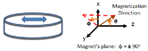
Figure 1: A nanomagnet shaped like an elliptical cylinder. The nanomagnet cross-sections are on the y-z plane. The magnetization direction can be rotated with a spin polarized current.

The magnetization M(t) of the single-domain nanomagnet has a constant magnitude but a variable orientation, so that we can represent it by the vector of unit norm $\mathbf{n_{m}}(t)=\mathbf{M}(t)/|\mathbf{M}|=\mathbf{\hat{e}_{r}}$ where $\mathbf{\hat{e}_{r}}$ is the unit vector in the radial direction. The other two unit vectors are denoted by $\mathbf{\hat{e}_{\theta}}$ and $\mathbf{\hat{e}_{\phi}}$ for $\theta$ and $\phi$ rotations, respectively.

The torque acting on the magnetization within unit volume due to shape anisotropy is Roy et al. (2011)

$$\mathbf{T_{E}}(t) = -\mathbf{\hat{e}_{r}}\times\nabla E(\theta(t),\phi(t))$$

$$= -\{2B(t)sin\theta(t)cos\theta(t)\}\mathbf{\hat{e}_{\phi}}-\{B_{0e}(t)\,sin\theta(t)\}\mathbf{\hat{e}_{\theta}},$$

(3)

where

$$B_{0e}(t)=B_{0e}(\phi(t))=\frac{\mu_{0}}{2}\,M_{s}^{2}\Omega(N_{d-xx}-N_{d-yy})sin(2\phi(t)).$$ (4)

Passage of a constant spin-polarized current $I$ perpendicular to the plane of the nanomagnet generates a spin-transfer-torque that is given by Roy et al. (2011)

$$\mathbf{T_{STT}}(t)=s\,\left[c_{s}(V)\,sin\theta(t)\,\mathbf{\hat{e}_{\theta}}-b_{s}(V)\,sin\theta(t)\,\mathbf{\hat{e}_{\phi}}\right],$$ (5)

where $s=(\hbar/2e)\eta I$ is the spin angular momentum deposition per unit time and $\eta$ is the degree of spin-polarization in the current $I$. The coefficients $b_{s}(V)$ and $c_{s}(V)$ are voltage-dependent dimensionless terms that arise when the nanomagnet is coupled with an insulating layer as in an MTJ Salahuddin et al. (2008) and the spin-polarized current tunnels through this layer. We will use constant values of $b_{s}(V)$ and $c_{s}(V)$ for simplicity Nikonov et al. (2010). Furthermore, we will assume $b_{s}(V)=0.3\,|c_{s}(V)|$ and $|c_{s}(V)|=1$ to be in approximate agreement with the experimental results presented in Refs. [Kubota et al., 2008, Sankey et al., 2008]. For $\theta$ = 180^∘ to 0^∘ switching, $c_{s}(V)=+1$, and for $\theta$ = 0^∘ to 180^∘ switching, $c_{s}(V)=-1$, while $b_{s}(V)=+0.3$ for both cases.

The magnetization dynamics of the single-domain nanomagnet under the action of various torques is described by the Landau-Lifshitz-Gilbert (LLG) equation as

$$\frac{d\mathbf{n_{m}}(t)}{dt}-\alpha\left(\mathbf{n_{m}}(t)\times\frac{d\mathbf{n_{m}}(t)}{dt}\right)=-\frac{|\gamma|}{M_{V}}\,\mathbf{T_{eff}}(t)$$ (6)

where $\mathbf{T_{eff}}(t)=\mathbf{T_{E}}(t)+\mathbf{T_{STT}}(t)$, $\alpha$ is the dimensionless phenomenological Gilbert damping constant, $\gamma=2\mu_{B}\mu_{0}/\hbar$ is the gyromagnetic ratio for electrons, and $M_{V}=\mu_{0}M_{s}\Omega$. Using spherical coordinate system, with constant magnitude of magnetization, we get the following coupled equations for the dynamics of $\theta(t)$ and $\phi(t)$:

$$\left(1+\alpha^{2}\right)\frac{d\theta(t)}{dt}=\frac{|\gamma|}{M_{V}}[\{-s\left(c_{s}(V)+\alpha\,b_{s}(V)\right)\\ +B_{0e}(t)\}sin\theta(t)-2\alpha B(t)sin\theta(t)cos\theta(t)]$$ (7)

$$\left(1+\alpha^{2}\right)\frac{d\phi(t)}{dt}=\frac{|\gamma|}{M_{V}}[\{s\left(b_{s}(V)-\alpha\,c_{s}(V)\right)+\alpha B_{0e}(t)\}\\ +2B(t)cos\theta(t)]\qquad(sin\theta\neq 0).$$ (8)

Note that when the magnetization vector is aligned along the easy axis (i.e. $\theta=0^{\circ},180^{\circ}$), the torque due to shape anisotropy, $\mathbf{T_{E}}(t)$ and the torque due to spin-transfer-torque, $\mathbf{T_{STT}}(t)$ both vanish (see Equations (3) and (5)), which makes $d\theta(t)/dt$ as well as $d\phi(t)/dt$ equal to zero. Hence the two mutually anti-parallel orientations along the easy axis become “stable”. If the magnetization is in either of these states, no amount of switching current $I$ can budge it (because the spin-transfer-torque vanishes), which is why these two orientations are also referred to as “stagnation points”. Fortunately, thermal fluctuations can dislodge the magnetization from a stagnation point and enable switching. We will now show that there can be a third set of values $(\theta_{3},\phi_{3})$ for $\theta(t)$ and $\phi(t)$ for which both $d\theta(t)/dt$ and $d\phi(t)/dt$ will vanish.

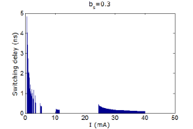
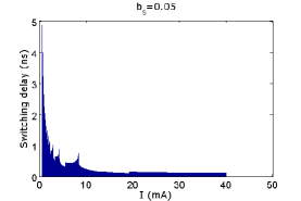
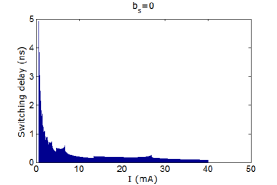
Figure 2: Switching delays for a range of switching current 700 $\mu$A – 40 mA producing spin-transfer-torque for $c_{s}(V)=-1$ and different values of $b_{s}(V)$. The switching current is varied in steps of 10 $\mu$A. (a) $b_{s}(V)=0.3$. No switching occurs for the following switching current ranges: 2-2.05 mA, 2.33-2.49 mA, 2.83–3.26 mA, 3.69–5.09 mA, 5.6–10.24 mA, 11.41–24.51 mA. The switching failure is either due to the metastable state or the magnetization vector ending up in a state where it stops rotating and begins to oscillate around a mean orientation. The latter is a different state not discussed here. (b) $b_{s}(V)=0.05$. Switching succeeds for the entire range of switching current. Metastable state appears for $b_{s}(V)>0.05$. (c) $b_{s}(V)=0$. Switching succeeds for the entire range of switching current.

We determine the values of $(\theta_{3},\phi_{3})$ as follows. From Equations (7) and (8), by making both $d\theta(t)/dt$ and $d\phi(t)/dt$ equal to zero, we get

$$2\alpha B(\phi_{3})cos\theta_{3} =B_{0e}(\phi_{3})-s\,c_{s}(V)-\alpha s\,b_{s}(V)$$ (9)

$$2B(\phi_{3})cos\theta_{3} =-\alpha B_{0e}(\phi_{3})+\alpha s\,c_{s}(V)-s\,b_{s}(V).$$ (10)

From the above two equations, we get $B_{0e}(\phi_{3})=sc_{s}(V)$. If we put $B_{0e}(\phi_{3})=sc_{s}(V)$ in Equation (9) or in Equation (10), we get $2B(\phi_{3})cos\theta_{3}=-sb_{s}(V)$. Accordingly, we can determine the values of $(\theta_{3},\phi_{3})$ as

$$\phi_{3} =\cfrac{1}{2}\,sin^{-1}\left(\cfrac{(\hbar/2e)\eta Ic_{s}(V)}{(\mu_{0}/2)\,M_{s}^{2}\Omega(N_{d-xx}-N_{d-yy})}\right)$$ (11)

$$\theta_{3} =cos^{-1}\left(-\cfrac{(\hbar/2e)\eta Ib_{s}(V)\left[\mu_{0}M_{s}^{2}\Omega\right]^{-1}}{N_{d-xx}cos^{2}\phi_{3}+N_{d-yy}sin^{2}\phi_{3}-N_{d-zz}}\right).$$ (12)

Note that $\phi_{3}$ depends on $c_{s}(V)$ while $\theta_{3}$ depends on both $c_{s}(V)$ and $b_{s}(V)$. Neither depends on the Gilbert damping factor $\alpha$.

In order to understand the physical origin of the state $(\theta_{3},\phi_{3})$, consider the fact that the total torque $\mathbf{T_{eff}}(t)=\mathbf{M}(t)\times\mathbf{H_{eff}}(t)$ can be deduced from Equations (3) and (5) as

$$\mathbf{T_{eff}}(t) = \left\{-2B(t)cos\theta(t)-sb_{s}(V)\right\}sin\theta(t)\,\mathbf{\hat{e}_{\phi}}$$ (13)

$$+\left\{-B_{0e}(t)+sc_{s}(V)\right\}sin\theta(t)\,\mathbf{\hat{e}_{\theta}}.$$

We immediately see that $\mathbf{T_{eff}}(t)$ vanishes when $\theta(t)=\theta_{3}$ and $\phi(t)=\phi_{3}$. Hence there is no torque acting on the magnetization vector if it reaches the state $\theta(t)=\theta_{3}$ and $\phi(t)=\phi_{3}$ at the same instant of time $t$. Thereafter, it cannot rotate any further since the torque has vanished. Unlike in the case of the other two stable states where both shape-anisotropy torque and spin-transfer-torque individually vanish, here neither vanishes, but they are equal and opposite so that they cancel to make the net torque zero. If the magnetization ends up in this orientation, then it will be stuck and not rotate further unless we change the switching current $I$ to change the spin-transfer-torque. Since changing $I$ can dislodge the magnetization from this state, it is not a stagnation point unlike $\theta=0^{\circ},180^{\circ}$. Hence, we call it a “metastable” state.

If $b_{s}(V)=0$, then $\theta_{3}=90^{\circ}$, which means that the magnetization will be stuck somewhere in the x-y plane perpendicular to the easy axis, if it lands in the metastable state. This plane is defined by the in-plane and out-of-plane hard axes. Note that when $c_{s}(V)$ is negative, $\phi_{3}$ is in the range $-90^{\circ}\leq\phi_{3}\leq 0^{\circ}$, but when $c_{s}(V)$ is positive, $0^{\circ}\leq\phi_{3}\leq 90^{\circ}$. The quantity $b_{s}(V)$ cannot be negative Salahuddin et al. (2008). Note also that when $I$ = 0 so that there is no spin-transfer-torque, $\theta_{3}$ = 90^∘ and $\phi_{3}$ can be any of the following values: $\{0^{\circ},90^{\circ},180^{\circ},270^{\circ}\}$. Consequently, the magnetization vector is either along the in-plane hard axis (y-axis) or the out-of-plane hard axis (x-axis). Since these are obviously metastable states in an unperturbed shape-anisotropic nanomagnet, we call the state $\left(\theta_{3},\phi_{3}\right)$ a “metastable” state.

For numerical simulations, we consider a nanomagnet of elliptical cross-section made of CoFeB alloy which has saturation magnetization $M_{s}=8\times 10^{5}$ A/m Fidler and Schrefl (2000) and a Gilbert damping factor $\alpha$ = 0.01. We assume the lengths of major axis ($a$), minor axis ($b$), and thickness ($l$) to be 150 nm, 100 nm, and 2 nm, respectively. These dimensions ($a$, $b$, and $l$) ensure that the nanomagnet will consist of a single ferromagnetic domain Beleggia et al. (2005); Cowburn et al. (1999). The combination of the parameters $a$, $b$, $l$, and $M_{s}$ makes the in-plane shape anisotropy energy barrier height $\sim$32 kT at room temperature. With the dimensions ($a$, $b$, and $l$) chosen, the demagnetization factors ($N_{d-xx}$,$N_{d-yy}$,$N_{d-zz}$) turn out to be (0.947,0.034,0.019) Beleggia et al. (2005). The spin polarization of the switching current is always assumed to be 80%.

We assume that the magnetization is initially along the +z-axis, which is a stagnation point. Hence, at 0 K, no switching can occur. However, at a finite temperature, thermal fluctuations will dislodge the magnetization from the stagnation point and enable switching. At room temperature, the thermal fluctuations will deflect the magnetization vector by $\sim$4.5^∘ from the easy axis when averaged over time Roy et al. (2011), so that we will assume the initial value of the polar angle to be $\theta_{init}$ = $4.5^{\circ}$. We choose the initial azimuthal angle $\phi_{init}$ as $+90^{\circ}$ because it is the most likely value in the absence of spin transfer torque. Similar assumptions are made by others Nikonov et al. (2010). We then solve Equations (7) and (8) simultaneously to find $\theta(t)$ and $\phi(t)$ as a function of time. Once $\theta(t)$ reaches $175.5^{\circ}$, regardless of the value of $\phi(t)$, we consider the switching to have completed. The time taken for this to happen is the switching delay.

Fig. 2 shows the switching delays versus switching current for different values of $b_{s}(V)$. The switching delay is ‘infinity’ in some current ranges when $b_{s}(V)=0.03$ because switching failed [see Fig. 2]. However, beyond the current of 24.51 mA, switching always occurs within a finite time, meaning that the magnetization never ends up in the metastable state. Simulation results show that if the value of $b_{s}$ is small enough ($\leq 0.05$), the metastable state does not show up [see Figs. 2 and 2].

The important question is why switching fails only for certain ranges of the current $I$, i.e. why does the magnetization vector land in the metastable state for certain values of $I$ and not others? The answer is that starting from some initial condition $\left(\theta_{init},\phi_{init}\right)$, the angles $\theta(t)$ and $\phi(t)$ must reach the values $\theta_{3}$ and $\phi_{3}$ at the same instant of time $t$. This may not happen for any arbitrary $I$. Hence, only certain ranges of $I$ will spawn the metastable state. It is also clear from Equation (11) that above a certain value of $I$, there will be no real solution for $\phi_{3}$ since the argument of the arcsin function will exceed unity. This value will be $I_{threshold}=\left[e\mu_{0}M_{s}^{2}\Omega\left(N_{d-xx}-N_{d-yy}\right)\right]/\left[\hbar\eta c_{s}(V)\right]$. By maintaining the magnitude of the switching current above $I_{threshold}$, we can ensure that the magnetization vector will never get stuck at the metastable state. For the nanomagnet considered, $I_{threshold}$ = 32.7 mA, but switching becomes feasible at even lower current of 24.52 mA since in the range [24.52 mA, 32.7 mA], the coupled $\theta$ and $\phi$-dynamics expressed by Equations (7) and (8) do not allow $\theta(t)$ and $\phi(t)$ to reach $\theta_{3}$ and $\phi_{3}$ simultaneously starting from $\left(\theta_{init},\phi_{init}\right)$.

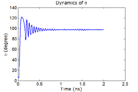
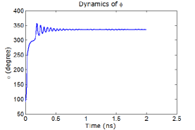
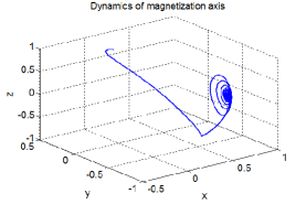
Figure 3: Room-temperature (300 K) magnetization dynamics when the switching current is 24.51 mA ($c_{s}(V)=-1$, $b_{s}(V)=0.3$). (a) Dynamics of $\theta(t)$. (b) Dynamics of $\phi(t)$. (c) The trajectory traced out by the tip of the magnetization vector in three-dimensional space. The magnetization gets stuck at a metastable state with $\theta_{3}$ = 97.58^∘ and $\phi_{3}$ = 335.87^∘. This plot was obtained by the solution of the stochastic Landau-Lifshitz-Gilbert equation in the presence of a random thermal torque to simulate the effect of thermal fluctuations Roy et al. (2011). This is one specific run from 10,000 simulations performed in the presence of thermal fluctuations that shows that the latter cannot untrap the magnetization from this state at room temperature. This happens for all the 10,000 simulations if thermal fluctuations are brought into play after the metastable state is reached. This shows that the state is stable against room-temperature thermal perturbations.

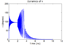
Figure 4: Time evolution of $\theta(t)$ when the switching current is 20 mA ($c_{s}(V)=-1$, $b_{s}(V)=0.3$). Thermal fluctuations were ignored but we assumed $\theta_{init}=4.5^{\circ}$ and $\phi_{init}=90^{\circ}$, respectively. The switching current is turned off at 2 ns after the magnetization vector gets stuck at the metastable state with $\theta_{3}$ = 95.74^∘ and $\phi_{3}$ = 341.25^∘. The dynamics shows that the magnetization vector relaxes to the easy axis because of shape anisotropy, but the final orientation is the wrong orientation along the +z-axis rather than the desired final orientation along the -z-axis. Therefore, switching fails.

Another important question is whether thermal fluctuations can untrap the magnetization from this state. To probe this, we solved the stochastic LLG equation Roy et al. (2011) in the presence of a random thermal torque. Fig. 3 shows the magnetization dynamics for a switching current of 24.51 mA at room temperature (300 K). We observe that the magnetization gets stuck at a metastable state (with $\theta_{3}$ = 97.58^∘ and $\phi_{3}$ = 335.87^∘) $\sim$50% of the time, which means that roughly one-half of the switching trajectories intersect the metastable state and terminate there. The values of $\theta_{3}$, $\phi_{3}$ are also the angles predicted by Equations (11) and (12), thereby confirming that the metastable state indeed has the origin described here. Increasing the temperature to 400 K helps by decreasing the probability that a switching trajectory will intersect the metastable state sup . What is important however is that if the magnetization vector gets stuck in the metastable state and the current remains on, then no amount of thermal fluctuations can dislodge it. In other words, this state is stable against thermal perturbations.

Unfortunately, an analytical stability analysis is precluded by the complex coupled $\theta$-$\phi$ dynamics. Therefore, we performed numerical stability analysis while spanning the parameter space as exhaustively as possible. In all cases, we found the state to be stable against thermal agitations.

We also notice that oscillations precede settling into the metastable state. This is due to coupled $\theta$- and $\phi$-dynamics governing the rotation of the magnetization vector, which causes some ringing. The metastable state appears in the switching current range 11.41 mA to 24.51 mA since within this range, $\theta(t)$ and $\phi(t)$ can reach $\theta_{3}$ and $\phi_{3}$ simultaneously starting with the initial conditions $\left(\theta_{init},\phi_{init}\right)$. If the initial conditions are changed, the range can change as well sup .

Finally, one issue that merits discussion is what happens if the spin polarized current is turned off after the magnetization gets stuck. In that case, the torque due to shape anisotropy will take over and drive the magnetization to the easy axis. One expects that if $\theta_{3}<90^{\circ}$, then switching will fail since the nearer easy axis is the undesired orientation, whereas if $\theta_{3}>90^{\circ}$, then switching should succeed because the nearer easy axis is the desired orientation. Equation (12) dictates that $\theta_{3}>90^{\circ}$ since $b_{s}(V)$ is always positive. Unfortunately, these simple expectations are belied by the complex dynamics of magnetization. The out-of-plane excursion of the magnetization vector causes an additional torque that depends on $\theta_{3}$, $\phi_{3}$. The torque can oppose the torque due to shape anisotropy. As a result, even when $\theta_{3}>90^{\circ}$, switching can fail since the magnetization reaches the wrong orientation along the easy axis (see Fig. 4).

In conclusion, we have shown the existence of a new metastable magnetization state in a single-domain nanomagnet with uniaxial shape anisotropy carrying a spin-polarized current. If the magnetization gets trapped in this state, switching will fail with non-zero probability even in the presence of thermal fluctuations. This has vital implications for STT-RAM technology.

References

- Slonczewski (1996) J. C. Slonczewski, J. Magn. Magn. Mater. 159, L1 (1996).
- Sun (2000) J. Z. Sun, Phys. Rev. B 62, 570 (2000).
- Chappert et al. (2007) C. Chappert, A. Fert, and F. N. V. Dau, Nature Mater. 6, 813 (2007).
- Roy et al. (2011) K. Roy, S. Bandyopadhyay, J. Atulasimha, K. Munira, and A. Ghosh, arXiv:1107.0387 (2011).
- Chikazumi (1964) S. Chikazumi, Physics of Magnetism (Wiley New York, 1964).
- Salahuddin et al. (2008) S. Salahuddin, D. Datta, and S. Datta, arXiv:0811.3472 (2008).
- Nikonov et al. (2010) D. E. Nikonov, G. I. Bourianoff, G. Rowlands, and I. N. Krivorotov, J. Appl. Phys. 107, 113910 (2010).
- Kubota et al. (2008) H. Kubota, A. Fukushima, K. Yakushiji, T. Nagahama, S. Yuasa, K. Ando, H. Maehara, Y. Nagamine, K. Tsunekawa, and D. D. Djayaprawira, Nature Phys. 4, 37 (2008).
- Sankey et al. (2008) J. C. Sankey, Y. T. Cui, J. Z. Sun, J. C. Slonczewski, R. A. Buhrman, and D. C. Ralph, Nature Phys. 4, 67 (2008).
- Fidler and Schrefl (2000) J. Fidler and T. Schrefl, J. Phys. D: Appl. Phys. 33, R135 (2000).
- Beleggia et al. (2005) M. Beleggia, M. D. Graef, Y. T. Millev, D. A. Goode, and G. Rowlands, J. Phys. D: Appl. Phys. 38, 3333 (2005).
- Cowburn et al. (1999) R. P. Cowburn, D. K. Koltsov, A. O. Adeyeye, M. E. Welland, and D. M. Tricker, Phys. Rev. Lett. 83, 1042 (1999).
- (13) See supplementary material at ……………… for additional simulation results .