A New Model for Gamma-Ray Cascades in Extragalactic Magnetic Fields

Abstract

Very-high-energy (VHE, $E\gtrsim 100$ GeV) gamma rays emitted by extragalactic sources, such as blazars, initiate electromagnetic cascades in the intergalactic medium. The cascade photons arrive at the earth with angular and temporal distributions correlated with the extragalactic magnetic field (EGMF). We have developed a new semi-analytical model of the cascade properties which is more accurate than previous analytic approaches and faster than full Monte Carlo simulations. Within its range of applicability, our model can quickly generate cascade spectra for a variety of source emission models, EGMF strengths, and assumptions about the source livetime. In this Letter, we describe the properties of the model and demonstrate its utility by exploring the gamma-ray emission from the blazar RGB J0710+591. In particular, we predict, under various scenarios, the VHE and high-energy (HE, 100 MeV $\lesssim$ E $\lesssim$ 300 GeV) fluxes detectable with the VERITAS and Fermi Large Area Telescope (LAT) observatories. We then develop a systematic framework for comparing the predictions to published results, obtaining constraints on the EGMF strength. At a confidence level of 95%, we find the lower limit on the EGMF strength to be $\sim 2\times 10^{-16}$ Gauss if no limit is placed on the livetime of the source or $\sim 3\times 10^{-18}$ Gauss if the source livetime is limited to the past $\sim$ 3 years during which Fermi observations have taken place.

1. Introduction

The extragalactic magnetic field (EGMF) is of great interest to the overall understanding of astrophysical magnetic fields and related processes. It could act as a seeding field for magnetic fields in galaxies and clusters (Widrow 2002), and its origin may be related to inflation or other periods in the early history of the universe (Grasso & Rubinstein 2001). Faraday rotation measurements (Kronberg & Perry 1982; Kronberg 1994; Blasi et al. 1999) and analysis of COBE data anisotropy (Barrow et al. 1997; Durrer et al. 2000) have put an upper bound on the EGMF strength at $\sim 10^{-9}$ Gauss. On the other hand, gamma-ray-initiated electromagnetic cascades deflected by the EGMF in intergalactic space have a characteristic angular spread (Aharonian et al. 1994) and time delay (Plaga 1995), both of which provide a probe for lower EGMF strengths (Neronov & Semikoz 2007; Elyiv et al. 2009). Present and next generation gamma-ray telescopes have the possibility to measure the EGMF strength by observing the angular and temporal distributions of cascade photons from extragalactic gamma-ray sources such as blazars (Neronov & Semikoz 2009; Dolag et al. 2009).

With current very-high-energy (VHE, $E\gtrsim 100$ GeV) and high-energy (HE, 100 MeV $\lesssim E\lesssim 300$ GeV) gamma-ray data on VHE-selected blazars, a lower limit on the EGMF strength can be placed by requiring that the cascade flux of VHE emission not exceed the measured flux or upper limit in the HE band (Murase et al. 2008; Neronov & Vovk 2010). Analytic cascade models assuming a simple relationship between the cascade flux and EGMF strength have put the lower limit at $10^{-16}$ to $10^{-15}$ Gauss when the source livetime is unlimited (Tavecchio et al. 2010, 2011; Neronov & Vovk 2010), similar to the results of Monte Carlo simulations (Dolag et al. 2011; Taylor et al. 2011). If the cascade time delay is limited to the $\sim 3$ years of simultaneous HE and VHE observations, the lower limit becomes $10^{-19}$ to $10^{-18}$ Gauss according to the simple cascade models (Dermer et al. 2011), or $10^{-18}$ to $10^{-17}$ Gauss according to the simulations (Taylor et al. 2011).

In this Letter, we present a new semi-analytic model of the electromagnetic cascade. In contrast to previous analytic cascade models (Dermer et al. 2011; Neronov & Semikoz 2009; Tavecchio et al. 2011), our cascade model considers the full track of the primary photon without the assumption of interacting exclusively at the mean free path. This simultaneously accounts for both angular and temporal constraints in a natural way. In addition, we model the radiation backgrounds and source emission in greater detail. As a complementary approach to full Monte Carlo simulations (Dolag et al. 2011; Taylor et al. 2011; Arlen et al. 2011), our model serves as a tool for clarifying the cascade picture, rapidly searching through the parameter space, and interpreting simulation results. We also develop a systematic framework for applying our cascade model’s predictions to derive lower limits on the EGMF strength at specific confidence levels. This framework is applicable to the results of Monte Carlo simulations as well.

2. Mathematical Model of Cascades

Consider a blazar emitting gamma rays at distance $L$. Gamma rays emitted at an angle $\theta_{s}$ relative to the line of sight may produce an $e^{\pm}$ pair via absorption on the photon background (Gould & Schréder 1967) at a distance $L^{\prime}$ from the source, not necessarily equal to the mean free path. After being deflected by the EGMF through the angle $\theta_{d}$, the pairs could scatter background photons to gamma-ray energies, redirecting them toward the observer. These secondary gamma rays would arrive at an incidence angle $\theta_{c}$ (see Fig. 1). In this picture, the influence of the EGMF enters solely through $\theta_{d}$. The angles $\theta_{c}$ and $\theta_{s}$ are uniquely specified in terms of $\theta_{d}$, $L$, and $L^{\prime}$, provided $\theta_{c}<\pi/2$.

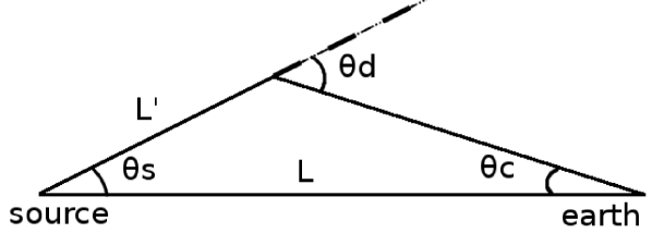
Figure 1.— Geometry used to calculate the gamma-ray cascade, following Dermer et al. (2011).

Because the energy density of CMB photons far exceeds that of the extragalactic background light (EBL), we assume that inverse Compton scattering proceeds in the Thomson regime via $e^{\pm}$ interactions with the CMB exclusively. An electron with Lorentz factor $\gamma_{e}$ will on average scatter secondary photons to energy $4\gamma_{e}^{2}\epsilon_{0}/3$, where $\epsilon_{0}\approx 0.64$ meV is the average CMB photon energy (Blumenthal & Gould 1970). The energy loss rate of the electron is

$$\frac{d\gamma_{e}m_{e}c^{2}}{dt}=-\frac{4}{3}\epsilon_{0}cn_{\textnormal{CMB}}\sigma_{T}\gamma_{e}^{2},$$ (1)

where $c$ is the speed of light, $n_{\textnormal{CMB}}\approx 411\text{ cm}^{-3}$ is the CMB photon density, and $\sigma_{T}\approx 6.65\times 10^{-25}\text{ cm}^{2}$ is the Thomson cross section. For an EGMF B perpendicular to the electron momentum $\textbf{{p}}_{e}$, the deflection rate in terms of the Larmor radius $r_{l}=\gamma_{e}m_{e}c^{2}/eB$ is

$$\frac{d\theta_{d}}{dt}=\frac{c}{r_{l}}=\frac{eB}{\gamma_{e}m_{e}c}.$$ (2)

Thus, when an electron’s Lorentz factor has changed from $\gamma_{e0}$ to $\gamma_{e}$, the electron will have been deflected by

$$\theta_{d0}(\gamma_{e0},\gamma_{e})=\frac{3}{8}\frac{eB}{\epsilon_{0}n_{\textnormal{CMB}}\sigma_{T}}\left(\frac{1}{\gamma_{e}^{2}}-\frac{1}{\gamma_{e0}^{2}}\right).$$ (3)

However, if the angle $\theta_{f}$ between B and $\textbf{{p}}_{e}$ is other than $\pi/2$, Eq. 3 should be generalized to

$$\theta_{d}(\gamma_{e0},\gamma_{e},\theta_{f})=\arccos\left(\sin^{2}\theta_{f}\cos\theta_{d0}+\cos^{2}\theta_{f}\right).$$ (4)

We use the full CMB black-body spectrum to determine the observed cascade spectrum. The number of secondary photons between energies $E$ and $E+dE$ produced by an electron that changes Lorentz factor from $\gamma_{e}+d\gamma_{e}$ to $\gamma_{e}$ is the number density of CMB photons between $3E/(4\gamma_{e}^{2})$ and $3(E+dE)/(4\gamma_{e}^{2})$ times the Thomson cross section and the distance travelled by the electron:

$$dN(E,\gamma_{e}) = cdt\sigma_{T}\frac{27\pi E^{2}}{8\gamma_{e}^{4}}\frac{dE}{h^{3}c^{3}\gamma_{e}^{2}(e^{3E/4(\gamma_{e}^{2}kT)}-1)}$$ (5)

$$= \frac{81\pi E^{2}m_{e}d\gamma_{e}}{32h^{3}c\gamma_{e}^{8}\epsilon_{0}n_{\textnormal{CMB}}}\frac{dE}{e^{3E/(4\gamma_{e}^{2}kT)}-1}$$

where $h$ is the Planck constant, $k$ the Boltzmann constant, and $T=2.73$ K the CMB temperature.

In terms of the mean free path $\lambda(\epsilon)=L/\tau(\epsilon)$ inferred from the optical depth $\tau(\epsilon)$ of the EBL, the probability for a photon of energy $\epsilon$ to be absorbed between $L^{\prime}$ and $L^{\prime}+dL^{\prime}$ is $e^{-L^{\prime}/\lambda(\epsilon)}dL^{\prime}/\lambda(\epsilon)$. Approximating both particles in the resulting pair to have initial energy $m_{e}\gamma_{e0}c^{2}=\epsilon/2$, we calculate the differential flux of observed secondary photons by integrating over $L^{\prime}$, $\epsilon$, and $\gamma_{e}$, and averaging over $\theta_{f}$:

$$\frac{dN(E)}{dE}=\int\frac{d\gamma_{e}81\pi E^{2}m_{e}}{16h^{3}c\gamma_{e}^{8}\epsilon_{0}n_{CMB}\left(e^{3E/(4\gamma_{e}^{2}kT)}-1\right)}$$ (6)

$$\times \int d\theta_{f}g(\theta_{f})\int d\epsilon\int dL^{\prime}\frac{e^{-L^{\prime}/\lambda(\epsilon)}}{\lambda(\epsilon)}f\left(\epsilon,\theta_{s}\right)$$

$$\times \exp\left(-\sqrt{L^{2}+L^{\prime 2}-2LL^{\prime}\cos(\theta_{d}-\theta_{c})}/\lambda(E)\right)$$

Here, $g(\theta_{f})$ is the probability distribution of $\theta_{f}$, equal to $\sin\theta_{f}$ for an EGMF uniformly distributed in direction, and $f(\epsilon,\theta_{s})$ is the intrinsic flux of the source, with $\theta_{s}=\theta_{d}-\theta_{c}$ from Fig. 1. The $1/2\pi$ factor from the $e^{\pm}$ being deflected into the surface of a cone with opening angle $\theta_{d}$ cancels the $2\pi$ enhancement from a similar effect at the source. We take the integral over $\theta_{f}$ from $0$ to $\pi/2$. The physical lower bound for the integration over the primary energy $\epsilon$ is $\epsilon_{\textnormal{min}}=2\gamma_{e}m_{e}c^{2}$. Nearly all of the photons above 200 TeV will be absorbed within 1 Mpc of the source, and the $e^{\pm}$ pairs will be isotropized by the strong field of the surrounding galaxy, resulting in negligible cascade contribution. We therefore adopt an upper limit of $\epsilon_{\textnormal{max}}=200$ TeV, suggesting an upper limit of $\epsilon_{\textnormal{max}}/2m_{e}c^{2}$ on the $\gamma_{e}$ integration. As a practical matter, we enforce a lower limit of $\gamma_{e}=10^{5}$ on the $\gamma_{e}$ integration, motivated by the CMB density becoming negligible at energies above 3 meV and our disinterest in the cascade spectrum below 100 MeV.

Observational effects enter Eq. 6 through limits on the $L^{\prime}$ integration. As seen in Fig. 1, we can express $\theta_{c}$ as

$$\theta_{c}=\arcsin\left(\frac{L^{\prime}}{L}\sin\theta_{d}\right)$$ (7)

so that a cut on $\theta_{c}$ translates directly into a cut on $L^{\prime}$. Similarly, the time delay $\Delta T$ of cascade photons may be written as

$$c\Delta T=L^{\prime}+\sqrt{L^{2}+L^{\prime 2}-2LL^{\prime}\cos(\theta_{d}-\theta_{c})}-L,$$ (8)

exchanging a limit on the source livetime $\Delta T$ for another constraint on $L^{\prime}$. We adopt the intersection of the $L^{\prime}$ cuts from Eqs. 7 and 8 in evaluating the cascade flux via Eq. 6.

We now briefly examine several assumptions made in the construction of this cascade model. (i) Exact energy distributions of pair production products are approximated as each having half the energy of the primary photon, as the cascade spectrum only weakly depends on the spectral distribution of pairs (Coppi & Aharonian 1997). (ii) The Thomson limit assumption, appropriate when $\sqrt{\epsilon_{0}E}\ll m_{e}c^{2}$ $\Rightarrow$ $E\ll 400$ TeV, certainly produces spectra valid for the range of existing TeV gamma-ray instruments. (iii) We assume the EGMF to be coherent over the cooling length of the electrons, at most a few Mpc for the most energetic electrons, making this assumption valid for coherence lengths $\lambda_{B}\gtrsim$ 1 Mpc. (iv) Only secondary cascade photons are considered. For observed photons above 100 MeV, the primary energy must be $\epsilon\gtrsim 2m_{e}c^{2}\sqrt{3\times(100\text{ MeV})/4\epsilon_{0}}\approx 400$ GeV. The requirement for third-generation photons is thus $\epsilon\gtrsim 2m_{e}c^{2}\sqrt{3\times(400\text{ GeV})/4\epsilon_{0}}\approx 25$ TeV. While a primary photon above this energy does produce higher-generation cascade photons, the power going into the higher generations is small for conventional blazar emission models, leading to negligible contribution from higher-order cascades (Tavecchio et al. 2011). (v) Cosmological effects enter the cascade model solely in the calculation of $\lambda(\epsilon)$. Cosmic expansion, energy redshift, EBL evolution, and other cosmological effects are ignored, limiting the application of the cascade model to nearby sources ($z\lesssim 0.2$), considering the $(1+z)^{4}$ radiation density evolution. (vi) We assume axial symmetry in the intrinsic emission $f(\epsilon,\theta_{s})$, following the current understanding of blazar emission, that is, boosted isotropic emission from hot blobs with the jet direction pointing toward the earth (Urry & Padovani 1995). (vii) The blazar intrinsic emission should be steady over the time interval $\Delta T$.

To get the predicted cascade flux from Eq. 6, we require a source emission model $f(\epsilon,\theta_{s})$. Motivated by models of blazars as relativistically beamed sources (Urry & Padovani 1995) we model the intrinsic emission as boosted isotropic emission,

$$f(\epsilon,\theta_{s}) = f_{0}\left(1-\beta\cos\theta_{s}\right)^{-\alpha-1}\epsilon^{-\alpha}e^{-\epsilon/E_{0}}$$ (9)

$$+ f_{0}\left(1+\beta\cos\theta_{s}\right)^{-\alpha-1}\epsilon^{-\alpha}e^{-\epsilon/E_{0}},$$

that is, a power law of index $\alpha$ boosted by the Lorentz factor $\Gamma=1/\sqrt{1-\beta^{2}}$ with an exponential cutoff energy $E_{0}$. The second term in Eq. 9 models the blazar counter jet, which we find does not significantly impact our result. To get a conservative estimate for the cascade flux, we employ the EBL model from Franceschini et al. (2008) which is relatively transparent for VHE gamma rays. Having no prior assumptions on the EGMF structure, we take $g(\theta_{f})=\sin\theta_{f}$ to calculate the cascade flux in Eq. 6.

3. Application of the Model to Blazar Data

We demonstrate the cascade model by investigating RGB J0710+591, a high-frequency-peaked BL Lacertae (HBL) object located at a redshift of $z=0.125$, for which simultaneous HE and VHE data are available with no variability observed (Acciari et al. 2010). In the VHE regime, we take the spectrum reported by Acciari et al. (2010), while to get the HE spectrum we analyze publicly available Fermi Large Area Telescope (LAT) data taken from a $\sim 3$-year period between 2008 August and 2011 January, using the Fermi Science Tools v9r18p6 and the P6_V3_DIFFUSE instrument response functions (IRFs), with models gll_iem_v02 for the galactic diffuse and isotropic_iem_v02 for the isotropic background. Accounting for nearby point sources, we perform an unbinned likelihood analysis to get the spectrum between 100 MeV and 300 GeV, finding a best-fit index of $1.62\pm 0.11$. Next, we bin the data into five energy bins, demanding that each bin have a test statistic greater than 10 and a maximum relative uncertainty on the flux of $50\%$, as suggested by Abdo et al. (2010). The combined spectra appear in Fig. 2, demonstrating that the Fermi spectral points are consistent with the 68% confidence band from the unbinned likelihood analysis.

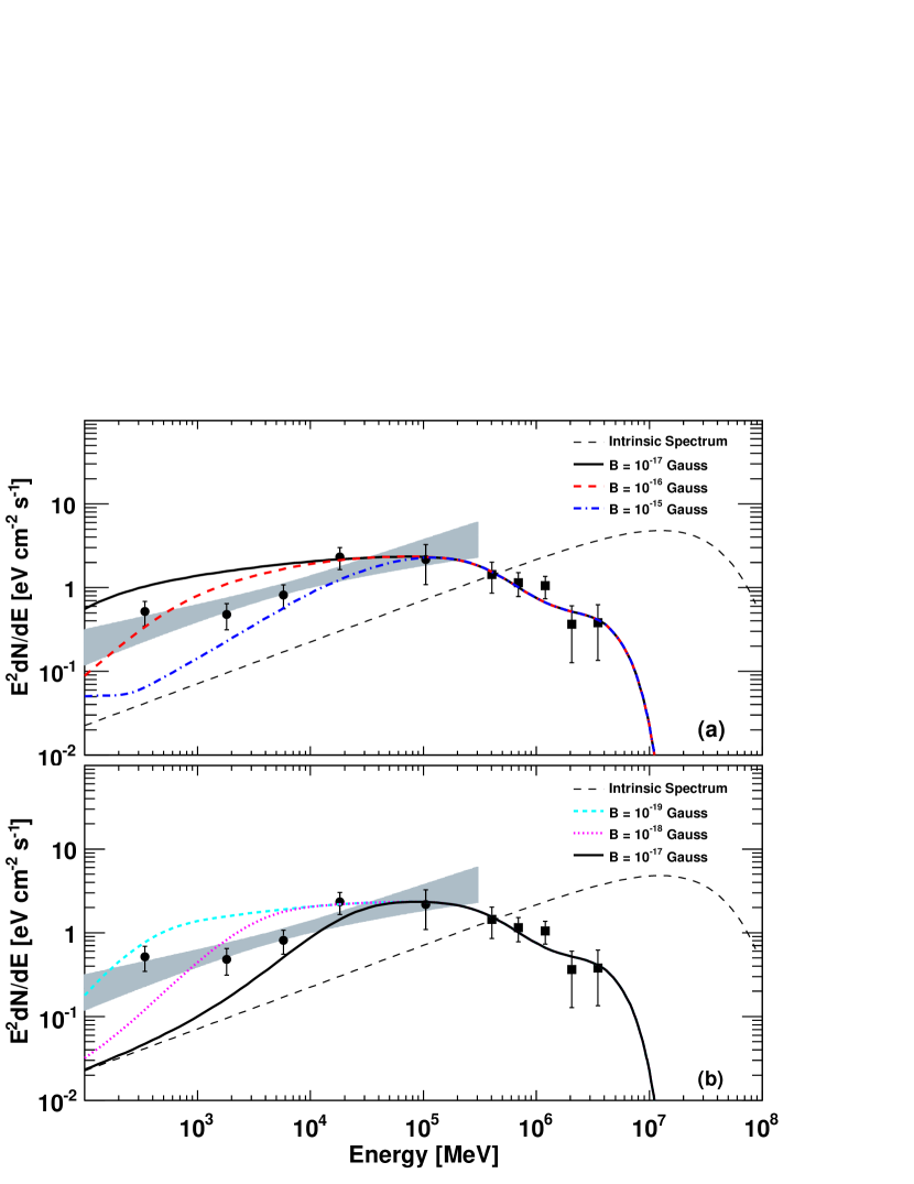
Figure 2.— Measured spectrum of RGB J0710+591 (points) and predictions for different situations (curves). Squares: VERITAS data points. Shaded area: Fermi 68% confidence band. Circles: Fermi data points. Panel a: Total fluxes for a source with unlimited livetime. Panel b: Total fluxes for a source with 3-year livetime.

To compare with the measured spectra, we compute the total flux as the sum of the cascade flux calculated by Eq. 6 and the direct flux $f(\epsilon,0)\exp\left(-\tau(\epsilon)\right)$, and then normalize it to observational data. For example, the results for $\alpha=1.5$, $E_{0}=25$ TeV, $\Gamma=10$, and a range of different EGMF strengths appear in Fig. 2(a) for a blazar with unlimited livetime, and in Fig. 2(b) for a blazar active for only 3 years. In both cases we require $\theta_{c}$ to be smaller than the 68% containment radius of the point spread function (PSF) (Atwood et al. 2009) in the Fermi range, or smaller than the $\theta^{2}$ cut (Acciari et al. 2010) in the VHE range. Setting the simple requirement that the flux be lower than the measured spectrum, we observe from Fig. 2 that the lower limit on the EGMF strength should be between $10^{-16}$ and $10^{-15}$ Gauss for the infinite-time case, and between $10^{-18}$ and $10^{-17}$ Gauss for the 3-year case, consistent with results shown by Taylor et al. (2011) for RGB J0710+591.

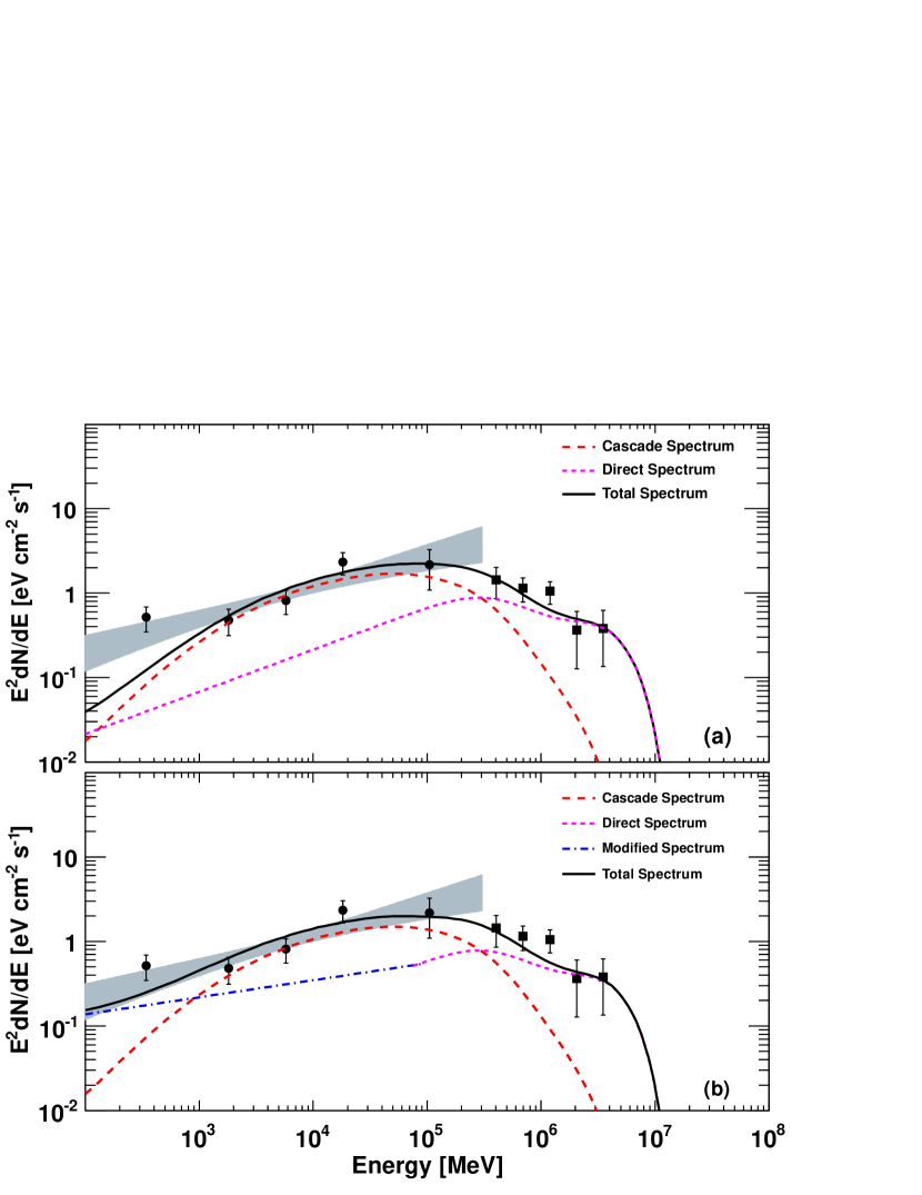
Figure 3.— Fitting RGB J0710+591 spectrum with cascade model predictions assuming unlimited source livetime. Squares: VERITAS data points. Shaded area: Fermi 68% confidence band. Circles: Fermi data points. Panel a: Fitting the sum of cascade flux and direct flux. Panel b: As Panel a, except the direct flux power-law index changes below 80 GeV (see text).

To be more rigorous, we fit the predicted flux to the data and use the resulting $\chi^{2}$ values to constrain the EGMF strength. Fig. 3(a) shows a sample fit for $\alpha=1.5$, $E_{0}=25$ TeV, $\Gamma=10$, and $B=3\times 10^{-16}$ Gauss. Because we cannot exclude the existence of additional components contributing to the blazar emission (e.g., Böttcher et al. 2008) and modifying the intrinsic spectrum of Eq. 9, we also fit a broken power law with an index $\alpha_{\text{break}}$ below 80 GeV, as shown for instance in Fig. 3(b). We find that the additional free parameter does not greatly affect our constraints on the EGMF.

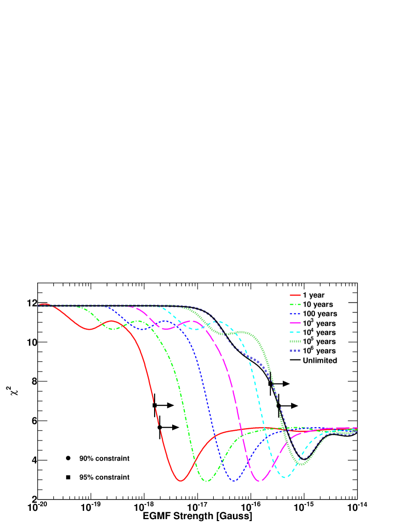
Figure 4.— Best-fit $\chi^{2}$ versus EGMF strength $B$ for various livetimes for RGB J0710+591. Lower limits on $B$ are indicated at 90% and 95% confidence levels for the 1-year and unlimited cases but omitted at intermediate times for clarity.

For each EGMF strength $B$, we find the best-fit model of the combined cascade and intrinsic emission for a wide range of cutoff energies $E_{0}\in(0.1$ TeV, 100 TeV), allowing $\alpha$ and $\alpha_{\text{break}}$ to vary between 2.5 and the physically motivated constraint of 1.5 (e.g., Malkov & O’C Drury 2001; Aharonian et al. 2006) and fixing $\Gamma$ to a typical value of 10. We plot the $\chi^{2}$ value of the best-fit model as a function of $B$ in Fig. 4 for blazar livetimes from 1 year to $10^{6}$ years, and for the unlimited case. At low $B$, the $\chi^{2}$ values converge because the cascade arrives promptly and at small angles. As $B$ increases, the arrival angles and times of the cascade begin to spread out, diminishing the observed emission and providing a better fit to the observed data.

The convergence of the curves in Fig. 4 to the infinite-livetime curve is easily understood. Combining Eq. 7 with Eq. 8 and assuming small angles, we can translate a cut on the instrument angle $\theta_{c}$ into a time cut $\Delta T_{c}$:

$$\Delta T_{c}\approx\frac{(L-L^{\prime})L}{2cL^{\prime}}{\theta_{c}}^{2}.$$ (10)

For example, source photons at 1 TeV, which have a mean free path of $L^{\prime}\approx 400$ Mpc, will produce cascade photons of energy $E\approx 0.8$ GeV, for which an angular cut of $\theta_{c}\approx 1^{\circ}$ is appropriate for the Fermi LAT. At the distance of RGB J0710+591 ($L\approx 500$ Mpc), this translates into a time cut of $\Delta T_{c}\approx 6\times 10^{4}$ years. This is close the the livetime of $\sim 10^{5}$ years at which the $\chi^{2}$ curves in Fig. 4 begin to converge to the unlimited-livetime case, becoming nearly indistinguishable at $\sim 10^{6}$ years. If the blazar livetime is smaller, the livetime cut outweighs the angle cut, and the position of the $\chi^{2}$ curve depends on the blazar livetime. For longer livetimes, the angle cut becomes more constraining and the curves converge to the unlimited-livetime case.

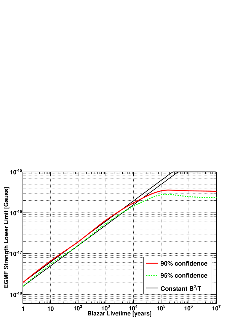
Figure 5.— Excluded field strength as a function of blazar livetime for two different confidence levels for RGB J0710+591. The solid black lines of constant $B^{2}/T$ agree with the curves for small times but begin to diverge for livetimes between $10^{4}$ and $10^{5}$ years, as expected. At longer times, the instrument PSF limits the possible delay time of the photons, causing the constraint to level off.

We constrain the EGMF strength for a given livetime by finding the point at which $\chi^{2}$ exceeds its minimum value by $\Delta\chi^{2}$ for each curve in Fig. 4. Two sample confidence levels (90% and 95%), corresponding to $\Delta\chi^{2}$ values of 2.72 and 3.84 (see e.g., James 2006) are indicated in the figure. The limits derived from these confidence levels are shown in Fig. 5 as a function of the blazar livetime. For livetimes below $\sim 10^{4}$ years, the limit on the EGMF strength scales with the blazar livetime $\Delta T$ as $B\sim\sqrt{\Delta T}$, as expected from combining Eq. 2 and Eq. 10. This relation breaks down when the time limit enforced by Eq. 10 is smaller than the blazar livetime. Our limit at 95% confidence is $B\gtrsim 2\times 10^{-16}$ Gauss if the blazar’s livetime is infinite and $B\gtrsim 3\times 10^{-18}$ Gauss if the livetime is 3 years, in agreement with the results of Taylor et al. (2011). In all cases, we reject the hypothesis of zero EGMF at greater than $2\sigma$ confidence.

4. Discussion and Conclusion

The cascade model we present builds upon previous models to give a more complete semi-analytic treatment, accounting for the photon trajectories, background spectra, and intrinsic emission in sufficient detail to produce realistic cascade predictions for different blazar livetimes. For example, the spectra shown in Fig. 2 converge to the zero field case at high energies and become suppressed by the field approximately as $1/B$ at low energies ($\sim 1$ GeV), in agreement with the spectra produced by a full Monte Carlo simulation as presented in Taylor et al. (2011). Previous cascade models (Tavecchio et al. 2010; Dermer et al. 2011) overestimate the suppression of the cascade flux in the EGMF compared to our result.

Combined with a systematic framework for interpreting the simultaneous fit of HE and VHE spectra to predictions, our model derives robust lower limits on the EGMF strength. The application of the model to RGB J0710+591 data yields lower limits at 95% confidence that agree with the results of Taylor et al. (2011) for the same source, further indicating that the physical picture of the cascade presented by the model is sufficiently complete to produce accurate results within the limits discussed in Sec. 2. The scaling of the lower limits with source livetime, depicted in Fig. 5, demonstrates that our analysis framework is also physically meaningful. The limits are conservative because we choose a low EBL model, as well as for a few other reasons that we now discuss.

We assume that the EGMF is configured as coherent domains of the same field strength and random field orientation, neglecting domain crossing by the $e^{\pm}$ pairs. In the energy range of interest, this restricts the domain size $\lambda_{B}$ to be $\lambda_{B}\gtrsim 1$ Mpc. If $\lambda_{B}\lesssim 1$ Mpc instead, domain crossing will result in smaller deflection angles for pairs (Ichiki et al. 2008; Neronov & Semikoz 2009) and a higher bound on the field strength than we report.

In testing various models of the intrinsic emission, we only consider cutoff energies below 100 TeV and spectral indices softer than 1.5. While it is possible to achieve intrinsic emission that is even harder by invoking some unconventional mechanism (e.g., Stecker et al. 2007; Böttcher et al. 2008; Aharonian et al. 2008), the HE cascade flux could only be higher in that case, leading to a more stringent lower limit. The spectral index could also be further constrained using multi-wavelength information (e.g., Tavecchio et al. 2011), which depends on detailed blazar modeling and hence is beyond the scope of this Letter.

The P6_V3_DIFFUSE IRFs used in the cascade model integration may underestimate the PSF at large energies (Ando & Kusenko 2010; Neronov et al. 2011), but Fig. 2 shows that the most constraining part of the HE spectrum for RGB J0710+591 is the low-energy region where this effect is small, and, as discussed in Sec. 3, it can only affect the cases with livetimes larger than $10^{4}$ years. Furthermore, we expect the IRFs we use to underestimate the cascade flux, so our lower limit is still conservative. In the future, there will be more realistic IRFs for the Fermi LAT, as well as more blazars with simultaneous HE-VHE baseline data available, and the lower limit could be further improved using the framework we present.

References

- Abdo et al. (2010) Abdo, A. A., et al. 2010, ApJS, 188, 405
- Acciari et al. (2010) Acciari, V. A., et al. 2010, ApJ, 715, L49
- Aharonian et al. (2006) Aharonian, F., et al. 2006, Nature, 440, 1018
- Aharonian et al. (1994) Aharonian, F. A., Coppi, P. S., & Voelk, H. J. 1994, ApJ, 423, L5
- Aharonian et al. (2008) Aharonian, F. A., Khangulyan, D., & Costamante, L. 2008, MNRAS, 387, 1206
- Ando & Kusenko (2010) Ando, S., & Kusenko, A. 2010, ApJ, 722, L39
- Arlen et al. (2011) Arlen, T., Huan, H., Vassiliev, V. V., Wakely, S. P., & Weisgarber, T. 2011, in preparation
- Atwood et al. (2009) Atwood, W. B., et al. 2009, ApJ, 697, 1071
- Barrow et al. (1997) Barrow, J. D., Ferreira, P. G., & Silk, J. 1997, Physical Review Letters, 78, 3610
- Blasi et al. (1999) Blasi, P., Burles, S., & Olinto, A. V. 1999, ApJ, 514, L79
- Blumenthal & Gould (1970) Blumenthal, G. R., & Gould, R. J. 1970, Reviews of Modern Physics, 42, 237
- Böttcher et al. (2008) Böttcher, M., Dermer, C. D., & Finke, J. D. 2008, ApJ, 679, L9
- Coppi & Aharonian (1997) Coppi, P. S., & Aharonian, F. A. 1997, ApJ, 487, L9+
- Dermer et al. (2011) Dermer, C. D., Cavadini, M., Razzaque, S., Finke, J. D., Chiang, J., & Lott, B. 2011, ApJ, 733, L21+
- Dolag et al. (2009) Dolag, K., Kachelrieß, M., Ostapchenko, S., & Tomàs, R. 2009, ApJ, 703, 1078
- Dolag et al. (2011) Dolag, K., Kachelriess, M., Ostapchenko, S., & Tomàs, R. 2011, ApJ, 727, L4+
- Durrer et al. (2000) Durrer, R., Ferreira, P. G., & Kahniashvili, T. 2000, Phys. Rev. D, 61, 043001
- Elyiv et al. (2009) Elyiv, A., Neronov, A., & Semikoz, D. V. 2009, Phys. Rev. D, 80, 023010
- Franceschini et al. (2008) Franceschini, A., Rodighiero, G., & Vaccari, M. 2008, A&A, 487, 837
- Gould & Schréder (1967) Gould, R. J., & Schréder, G. P. 1967, Physical Review, 155, 1408
- Grasso & Rubinstein (2001) Grasso, D., & Rubinstein, H. R. 2001, Phys. Rep., 348, 163
- Ichiki et al. (2008) Ichiki, K., Inoue, S., & Takahashi, K. 2008, ApJ, 682, 127
- James (2006) James, F. 2006, Statistical Methods in Experimental Physics: 2nd Edition, ed. James, F. (World Scientific Publishing Co)
- Kronberg (1994) Kronberg, P. P. 1994, Reports on Progress in Physics, 57, 325
- Kronberg & Perry (1982) Kronberg, P. P., & Perry, J. J. 1982, ApJ, 263, 518
- Malkov & O’C Drury (2001) Malkov, M. A., & O’C Drury, L. 2001, Reports on Progress in Physics, 64, 429
- Murase et al. (2008) Murase, K., Takahashi, K., Inoue, S., Ichiki, K., & Nagataki, S. 2008, ApJ, 686, L67
- Neronov & Semikoz (2007) Neronov, A., & Semikoz, D. 2007, JETP Letters, 85, 579
- Neronov & Semikoz (2009) Neronov, A., & Semikoz, D. V. 2009, Phys. Rev. D, 80, 123012
- Neronov et al. (2011) Neronov, A., Semikoz, D. V., Tinyakov, P. G., & Tkachev, I. I. 2011, A&A, 526, A90+
- Neronov & Vovk (2010) Neronov, A., & Vovk, I. 2010, Science, 328, 73
- Plaga (1995) Plaga, R. 1995, Nature, 374, 430
- Stecker et al. (2007) Stecker, F. W., Baring, M. G., & Summerlin, E. J. 2007, ApJ, 667, L29
- Tavecchio et al. (2011) Tavecchio, F., Ghisellini, G., Bonnoli, G., & Foschini, L. 2011, MNRAS, 570
- Tavecchio et al. (2010) Tavecchio, F., Ghisellini, G., Foschini, L., Bonnoli, G., Ghirlanda, G., & Coppi, P. 2010, MNRAS, 406, L70
- Taylor et al. (2011) Taylor, A. M., Vovk, I., & Neronov, A. 2011, A&A, 529, A144+
- Urry & Padovani (1995) Urry, C. M., & Padovani, P. 1995, PASP, 107, 803
- Widrow (2002) Widrow, L. M. 2002, Reviews of Modern Physics, 74, 775