Strong-coupling lattice study for QCD phase diagram
including both chiral and deconfinement dynamics

Abstract

We investigate the QCD phase diagram by using the strong-coupling expansion of the lattice QCD with one species of staggered fermion and the Polyakov loop effective action at finite temperature ($T$) and quark chemical potential ($\mu$). We derive an analytic expression of effective potential $\mathcal{F}_{\mathrm{eff}}$ including both the chiral ($U_{\chi}(1)$) and the deconfinement ($Z_{N_{c}}$) dynamics with finite coupling effects in the mean-field approximation. The Polyakov loop increasing rate ($d\ell_{p}/dT$) is found to have two peaks as a function of $T$ for small quark masses. One of them is the chiral-induced peak associated with the rapid decrease of the chiral condensate. The temperature of the other peak is almost independent of the quark mass or chemical potential, and this peak is interpreted as the $Z_{N_{c}}$-induced peak.

The phase diagram for chiral and deconfinement transitions in Quantum Chromodynamics (QCD) at finite temperature ($T$) and/or quark chemical potential ($\mu$) is one of the most fascinating subjects in the current high energy and nuclear physics. To investigate properties of QCD at high $T$ is one of the physics goals in the LHC-ALICE experiments. At $\mu=0$, first principle investigations based on lattice Monte-Carlo (LQCD-MC) simulations predict pseudo-critical temperature, $T_{c}\simeq 145-195~{}\mathrm{MeV}$, for the chiral phase transition [1]. In the finite $\mu$ region, the LQCD-MCs suffer from the notorious sign problem of the quark determinant, and have not provided reliable results in the large chemical potential region, $\mu/T>1$.

The strong-coupling ($1/g^{2}$) expansion in the lattice QCD (SC-LQCD) has been successful since the beginning of the lattice gauge theory, and would provide an alternative lattice framework to study the QCD phase diagram including finite $\mu$ region. In pure Yang-Mills theory, the string tension in the strong-coupling limit gives the area law [2], and the LQCD-MC [3] smoothly connects the strong-coupling result [4] to the scaling region. In the pure Yang-Mills theory at finite $T$, we can describe the $Z_{N_{c}}$ deconfinement transition based on the effective potential for the Polyakov-loop ($\ell_{p}$) in the leading order of the strong-coupling expansion with the Haar measure effects [5], and higher order corrections have been investigated recently [6]. For the SC-LQCD including fermions, many theoretical knowledge have been accumulated so far [7, 8, 9, 10, 11, 12, 13, 14, 15], and the chiral phase transition in the $T-\mu$ plane have been well investigated in the strong-coupling limit [16, 17, 18, 19]. It is remarkable that the coupling of the chiral condensate $\sigma$ and the Polyakov-loop $\ell_{p}$ was extracted in the strong-coupling limit [20, 21], and led to the invention of the Nambu-Jona-Lasino model with Polyakov-loops (PNJL model) [22]. Recently, the finite lattice couping ($\beta=2N_{c}/g^{2}$) effects are incorporated, and is found to give rise to modifications of quark mass and chemical potential. The evolution of the chiral phase transition with increasing $\beta$ has been interpreted via these modifications [23, 24]. As will be shown later, this development opens a possibility to investigate the finite coupling evolution of $Z_{N_{c}}$ deconfinement dynamics in addition to the chiral dynamics in the whole $T-\mu$ plane [25].

One of the interesting observations in the LQCD-MC is that peak positions of chiral and Polyakov loop susceptibilities ($\chi_{\sigma,\ell_{p}}$) are close to each other, and the small separation of them could be explained as a consequence of the broad analytic behavior of the crossovers [1]. It would be meaningful to ask ourselves whether the peak of $\chi_{\ell_{p}}$ is induced by the chiral crossover. Otherwise, does the $Z_{N_{c}}$ dynamics (accidentally or inevitably) leads to the peak of $\chi_{\ell_{p}}$ near the chiral crossover? To shed light on this problem, it is a good strategy to investigate the finite $\mu$ cases. In models such as PNJL model combined with the statistical model [26] or Polyakov-Quark Meson model with the functional renormalization group evolution [27], two transitions almost coincide. In the PNJL with a certain fit parameter set, the first-order chiral phase transition with a small jump of a small value of $\ell_{p}$ can be realized in the low $T$ and large $\mu$ region [28, 29, 30, 31].

In this Letter, we investigate the chiral and $Z_{N_{c}}$ deconfinement dynamics by using the SC-LQCD with the Polyakov loop effects, abbreviated as P-SC-LQCD. The P-SC-LQCD is directly based on the lattice QCD, and it does not contain any additional parameters than those in QCD. The lattice coupling $\beta=2N_{c}/g^{2}$ in the plaquette action is a unique parameter of the lattice QCD in the chiral limit. To investigate the chiral and $Z_{N_{c}}$ deconfinement dynamics simultaneously, we consider the effective action with leading [${\cal O}(1/g^{0})$] and next-to-leading order [NLO, ${\cal O}(1/g^{2})$] effects of the strong coupling expansion in the fermionic sector, and the leading order contributions to the Polyakov-loop [$\mathcal{O}(1/g^{2N_{\tau}})$] in the pure gluonic sector. The present framework aims at developing previous SC-LQCD studies for the chiral dynamics [11, 13, 16, 18, 23, 24] to include the $Z_{N_{c}}$ deconfinement dynamics, and leads to an extended version of the IK-GO model [20, 21] to include finite beta effects for the quark sector. This framework allows us to investigate the beta evolution of the interplay between chiral and $Z_{N_{c}}$ dynamics consistently. This is the advantage of using the P-SC-LQCD over effective models.

We briefly overview the derivation of the effective potential in P-SC-LQCD. Details are shown in our previous papers [23, 32]. We start from the lattice QCD partition function with one species of staggered fermion ($\chi$) with a current quark mass ($m_{0}$) in the lattice unit $a=1$,

$$\mathcal{Z}_{\mathrm{LQCD}} =\int\mathcal{D}[\chi,\bar{\chi},U_{\nu}]\exp\biggl{[}-S_{F}-S_{G}-m_{0}\sum_{x}\bar{\chi}_{x}\chi_{x}\biggr{]}\ ,$$ (1)

$$S_{F} =\frac{1}{2}\sum_{\nu,x}\Bigl{[}\eta_{\nu,x}\bar{\chi}_{x}U_{\nu,x}\chi_{x+\hat{\nu}}-\eta_{\nu,x}^{-1}(h.c.)\Bigr{]}\ ,$$ (2)

$$S_{G} =\beta\sum_{P}\biggl{[}1-\frac{1}{2N_{c}}\Bigl{[}U_{P}+U_{P}^{\dagger}\Bigr{]}\biggr{]}\ .$$ (3)

where $U_{\nu,x}\in SU(N_{c})$ and $U_{P=\mu\nu,x}=\mathrm{tr}_{c}[U_{\mu,x}U_{\nu,x+\hat{\mu}}U^{\dagger}_{\mu,x+\hat{\nu}}U^{\dagger}_{\nu,x}]$ represent the link-variable and plaquette, and the staggered sign factor $\eta_{\nu,x}=\exp(\mu\,\delta_{\nu 0})(-1)^{x_{0}+\cdots+x_{\nu-1}}$ contains the the lattice chemical potential $\mu$. The transformation $\chi_{x}\to e^{i\theta\epsilon_{x}}\chi_{x}$ with $\epsilon_{x}=(-1)^{x_{0}+\cdots+x_{d}}$ turns out to be a $U(1)_{\chi}$ chiral transformation [8, 10], which leaves the staggered action $S_{F}$ invariant in the chiral limit ($m_{0}\to 0$). The $U_{\chi}(1)$ chiral symmetry would be enhanced to $SU(N_{f}=4)$ in the continuum limit [10, 33, 34]. The plaquette action $S_{G}$ is invariant under the global transformation $U_{\nu,x}\to\Omega U_{\nu,x}$, where $\Omega$ is the element of the center of the $SU(N_{c})$ gauge group, $Z_{N_{c}}$. The chiral condensate ($\sigma\sim\langle\bar{\chi}\chi\rangle$) and the Polyakov-loop ($L_{p}=\mathrm{tr}_{c}(\prod_{\tau}U_{0,\mathbf{x}\tau})/N_{c}$) are the order parameters of the chiral and $Z_{N_{c}}$ symmetries, respectively, and they take finite values via the spontaneous breaking of these symmetries. Both chiral and $Z_{N_{c}}$ symmetries are explicitly broken for a finite quark mass $m_{0}$, and the transitions could be replaced with the crossovers. We concentrate on the color SU($N_{c}=3$) in the $3+1$ dimension ($d=3$) in the later discussion.

Figure 1: Effective action terms in the strong-coupling limit and $1/g^{2}$ corrections. Open circles, Filled circles, and arrows show $\chi$, $\bar{\chi}$, and $U_{\nu}$, respectively.

The effective action of hadronic composites is obtained by the Taylor expansion in $\beta$ and integrating out spatial link variables in the finite $T$ treatment of P-SC-LQCD. We include the leading and NLO terms in the fermionic sector, $\mathcal{S}_{\mathrm{eff}}^{\mathrm{NLO}}$ [23], and we adopt the leading order Polyakov-loop effective action $\mathcal{S}_{\mathrm{eff}}^{\mathrm{Pol}}$ in the pure gluonic sector [35],

$$\mathcal{Z}_{\mathrm{LQCD}}\simeq\int\mathcal{D}[\chi,\bar{\chi},U_{0}]~{}\exp\left(-\mathcal{S}_{\mathrm{eff}}^{\mathrm{NLO}}-\mathcal{S}_{\mathrm{eff}}^{\mathrm{Pol}}\right)\ ,$$ (4)

$$\mathcal{S}_{\mathrm{eff}}^{\mathrm{NLO}}=\sum_{x}\Biggl{[}\frac{1}{2}\left[V^{+}_{x}(\mu)-V^{-}_{x}(\mu)\right]+m_{0}M_{x}$$

$$~{}~{}~{}+\sum_{j>0}\biggl{[}-\frac{M_{x}M_{x+\hat{j}}}{4N_{c}}+\frac{\beta_{\tau}}{4d}\Bigl{[}V^{+}_{x}(\mu)V^{-}_{x+\hat{j}}(\mu)+V^{+}_{x}(\mu)V^{-}_{x-\hat{j}}(\mu)\Bigl{]}\biggr{]}$$

$$~{}~{}~{}-\frac{\beta_{s}}{d(d-1)}\sum_{0<k<j}M_{x}M_{x+\hat{j}}M_{x+\hat{k}}M_{x+\hat{k}+\hat{j}}\Biggr{]}+\mathcal{O}\biggl{(}\frac{1}{g^{4}},\frac{1}{\sqrt{d}}\biggr{)}\ ,$$ (5)

$$\mathcal{S}_{\mathrm{eff}}^{\mathrm{Pol}}[L_{p},\bar{L}_{p}]=-N_{c}^{2}\biggl{(}\frac{1}{g^{2}N_{c}}\biggr{)}^{N_{\tau}=1/T}\sum_{j,\mathbf{x}}\Bigl{[}\bar{L}_{p,\mathbf{x}}L_{p,\mathbf{x}+\hat{j}}+h.c.\Bigr{]}\ ,$$ (6)

where the coupling $\beta_{\tau,s}$ and composites are defined as $(\beta_{\tau},~{}\beta_{s})=(\beta d/2N_{c}^{3},~{}\beta d(d-1)/16N_{c}^{5})$, $M_{x}=\bar{\chi}_{x}\chi_{x}$, and $(V^{+}_{x}(\mu),~{}V^{-}_{x}(\mu))=(e^{\mu}\bar{\chi}_{x}U_{0,x}\chi_{x+\hat{0}},~{}e^{-\mu}\bar{\chi}_{x+\hat{0}}U_{0,x}^{\dagger}\chi_{x})$. We consider only the leading order terms in the $1/d$ expansion [9], which corresponds to the minimum quark number diagrams for a given plaquette configuration as shown in Fig. 1. $\mathcal{S}_{\mathrm{eff}}^{\mathrm{NLO}}$ contains the four-Fermi interaction, the temporal components of the vector interaction, and eight-Fermi interaction, and $\mathcal{S}_{\mathrm{eff}}^{\mathrm{Pol}}$ shows the nearest-neighbor interaction of the Polyakov loops. We can reduce the effective action $\mathcal{S}_{\mathrm{eff}}^{\mathrm{NLO}}$ into the bi-linear form in staggered fermions by introducing several auxiliary fields ($\sigma,~{}\omega_{\tau}$, and $\varphi_{\tau,s}$) summarized in Table 1,

$$\mathcal{S}_{\mathrm{eff}}^{\mathrm{NLO}}\simeq Z_{\chi}\sum_{xy}\bar{\chi}_{x}G_{xy}^{-1}(\tilde{m}_{q},\tilde{\mu})\chi_{y}$$

$$+N_{\tau}N_{s}^{d} \Biggl{[}\biggl{(}\frac{d}{4N_{c}}+\beta_{s}\varphi_{s}\biggr{)}\sigma^{2}+\frac{\beta_{s}}{2}\varphi_{s}^{2}+\frac{\beta_{\tau}}{2}\bigl{(}\varphi_{\tau}^{2}-\omega_{\tau}^{2}\bigr{)}\Biggr{]}\ ,$$ (7)

$$G_{xy}^{-1}(\tilde{m}_{q},\tilde{\mu})= \tilde{m}_{q}\delta_{xy}+\frac{\delta_{\mathbf{xy}}}{2}\Bigl{(}e^{\tilde{\mu}}U_{0,x}\delta_{x+\hat{0},y}-e^{-\tilde{\mu}}U_{0,x}^{\dagger}\delta_{x-\hat{0},y}\Bigr{)}\ ,$$ (8)

where $N_{\tau}$ ($N_{s}$) represents the temporal (spatial) lattice size, and all auxiliary fields are assumed to be constant and static. The spontaneous breaking of the chiral symmetry with NLO effects results in the dynamical shifts of quark mass $\tilde{m}_{q}=\left[m_{0}+\left(d/2N_{c}+2\beta_{s}\varphi_{s}\right)\sigma\right]/Z_{\chi}$, chemical potential $\tilde{\mu}=\mu-\log Z_{\chi}$, and the quark wave function renormalization factor, $Z_{\chi}$, where $Z_{\chi}=\sqrt{Z_{+}Z_{-}}$ and $Z_{\pm}=1+\beta_{\tau}(\varphi_{\tau}\pm\omega_{\tau})$. Such a property allows us to utilize the technique developed in the strong coupling limit, and from a technical point of view, it is essential to derive the effective potential including both the chiral and deconfinement dynamics.

Table 1: The auxiliary fields and their stationary values. Here, $\varphi_{0}=N_{c}-Z_{\chi}\tilde{m}_{q}+\beta_{\tau}\omega_{\tau}^{2}$.

Aux. Fields	Mean Fields	Stationary Values
$\sigma$	$\langle-M\rangle$	$-\partial{\cal V}_{q}/\partial(Z_{\chi}\tilde{m}_{q})$
$\varphi_{s}$	$\langle MM\rangle$	$\sigma^{2}$
$\varphi_{\tau}$	$-\langle(V^{+}-V^{-})/2\rangle$	$2\varphi_{0}/(1+\sqrt{1+4\beta_{\tau}\varphi_{0}})$
${\omega_{\tau}}$	$-\langle(V^{+}+V^{-})/2\rangle$	$-\partial{\cal V}_{q}/\partial\tilde{\mu}=\rho_{q}$

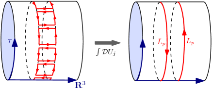
Figure 2: Schematic figure of the Polyakov-loop construction in the strong-coupling expansion.

Now we perform the Gaussian integral over the staggered quark fields $(\chi,\bar{\chi})$. Here we work in the static and diagonalized gauge (called the Polyakov gauge) for temporal link variables with respect for the periodicity [11],

$$\mathcal{U}_{0,\mathbf{x}}=\prod_{\tau}U_{0,\mathbf{x}\tau}=\mathrm{diag}\Bigl{\{}e^{i\theta_{1}(\mathbf{x})},\cdots,e^{i\theta_{N_{c}}(\mathbf{x})}\Bigr{\}}\ .$$ (9)

Owing to the static property of the auxiliary fields and the temporal link variable in the Polyakov gauge, the quark determinant is factorized in terms of the frequency modes, and evaluated by the Matsubara method (see for example the appendix in Ref. [18]). The remarkable point is that the resultant expression can be expressed in terms of the Polyakov-loop variables ($L_{p},\bar{L}_{p}$),

$$\int\mathcal{D}[\chi,\bar{\chi}]\exp\biggl{[}-Z_{\chi}\sum_{xy}\bar{\chi}_{x}G_{xy}^{-1}(\tilde{m}_{q},\tilde{\mu})\chi_{y}\biggr{]}$$

$$\quad=Z_{\chi}^{N_{c}N_{\tau}N_{s}^{d}}\prod_{\mathbf{x}}\Bigl{[}e^{N_{c}E_{q}/T}\mathcal{R}_{q}(T,\mu)\mathcal{R}_{\bar{q}}(T,\mu)\Bigr{]}\ ,$$ (10)

$$\mathcal{R}_{q}(T,\mu)\equiv 1+e^{-N_{c}(E_{q}-\tilde{\mu})/T}$$

$$\quad+N_{c}\Bigl{(}L_{p,\mathbf{x}}e^{-(E_{q}-\tilde{\mu})/T}+\bar{L}_{p,\mathbf{x}}e^{-2(E_{q}-\tilde{\mu})/T}\Bigr{)}\ ,$$ (11)

$$\mathcal{R}_{\bar{q}}(T,\mu)\equiv 1+e^{-N_{c}(E_{q}+\tilde{\mu})/T}$$

$$\quad+N_{c}\Bigl{(}\bar{L}_{p,\mathbf{x}}e^{-(E_{q}+\tilde{\mu})/T}+L_{p,\mathbf{x}}e^{-2(E_{q}+\tilde{\mu})/T}\Bigr{)}\ .$$ (12)

where $E(\tilde{m}_{q}(\sigma))=\sinh^{-1}\bigl{[}\tilde{m}_{q}(\sigma)\bigr{]}$ corresponds to the quark excitation energy. In that expression, $L_{p}$ couples to a Boltzmann factor $e^{-(E_{q}-\tilde{\mu})/T}$, and determines how quarks thermally excites. In the confined phase ($L_{p}\sim 0$), color-singlet states dominate, while quarks can excite in the deconfined phase ($L_{p}\neq 0$). Equations (11) and (12) give a natural coupling manner between $L_{p}$ and $\sigma$. This point has been pointed out in the strong-coupling limit [20, 21], and utilized in the PNJL model [22]. In the current formulation, the Boltzmann factor includes the NLO effects in $(\tilde{m}_{q},\tilde{\mu})$, and the coupling manner between $L_{p}$ and $\sigma$ is modified by the finite coupling effects.

Finally, we evaluate the temporal link integral and obtain the effective potential. In the Polyakov gauge, the Haar measure becomes a Van der Monde determinant over the color space, and can be rewritten by using the (reduced) Polyakov-loop ($L_{p,\mathbf{x}}\to\sum_{a=1}^{N_{c}}e^{i\theta_{a}(\mathbf{x})}/N_{c}$),

$$\int d\mathcal{U}_{0,\mathbf{x}}=27\int d[L_{p,\mathbf{x}},\bar{L}_{p,\mathbf{x}}]\mathcal{M}_{\mathrm{Haar}}(L_{p},\bar{L}_{p})\ ,$$ (13)

$$\mathcal{M}_{\mathrm{Haar}}(L_{p},\bar{L}_{p})=1-6\bar{L}_{p,\mathbf{x}}L_{p,\mathbf{x}}-3\bigl{(}\bar{L}_{p,\mathbf{x}}L_{p,\mathbf{x}}\bigr{)}^{2}+4\bigl{(}L_{p,\mathbf{x}}^{N_{c}}+\bar{L}_{p,\mathbf{x}}^{N_{c}}\bigr{)}\ .$$ (14)

While it is possible to perform this integral exactly, we here adopt a simpler prescription; we replace Polyakov-loops in the integrand with its constant mean-field value, $(L_{p,\mathbf{x}},\bar{L}_{p,\mathbf{x}})\to(\ell_{p},\bar{\ell}_{p})$, and search for the stationary values of $(\ell_{p},\bar{\ell}_{p})$. This treatment gives the effective potential in a similar expression to that used in the PNJL model, and useful for the comparison. Thus, we obtain the effective potential as a function of the auxiliary fields $\Phi=(\sigma,\varphi_{\tau,s},\omega_{\tau},\ell_{p},\bar{\ell}_{p})$, temperature $T$, and quark chemical potential $\mu$ in the mean-field approximation,

$$\mathcal{F}_{\mathrm{eff}}(\Phi;T,\mu)\equiv-(T\log\mathcal{Z}_{\mathrm{LQCD}})/N_{s}^{d}=\mathcal{F}_{\mathrm{eff}}^{\chi}+\mathcal{F}_{\mathrm{eff}}^{\mathrm{Pol}}\ ,$$ (15)

$$\mathcal{F}_{\mathrm{eff}}^{\chi}\simeq\biggl{(}\frac{d}{4N_{c}}+\beta_{s}\varphi_{s}\biggr{)}\sigma^{2}+\frac{\beta_{s}\varphi_{s}^{2}}{2}+\frac{\beta_{\tau}}{2}\bigl{(}\varphi_{\tau}^{2}-\omega_{\tau}^{2}\bigr{)}-N_{c}\log Z_{\chi}\ ,$$

$$~{}~{}~{}~{}~{}~{}~{}~{}~{}~{}-N_{c}E_{q}-T\bigl{(}\log\mathcal{R}_{q}(T,\mu)+\log\mathcal{R}_{\bar{q}}(T,\mu)\bigr{)}\ ,$$ (16)

$$\mathcal{F}_{\mathrm{eff}}^{\mathrm{Pol}}\simeq-2TdN_{c}^{2}\biggl{(}\frac{1}{g^{2}N_{c}}\biggr{)}^{1/T}\bar{\ell}_{p}\ell_{p}-T\log\mathcal{M}_{\mathrm{Haar}}(\ell_{p},\bar{\ell}_{p})\ ,$$ (17)

The equilibrium is determined by imposing stationary conditions on the effective potential, $\partial{\mathcal{F}_{\mathrm{eff}}}/\partial\Phi=0$, which lead to the relations summarized in the third column of Table 1. $\mathcal{F}_{\mathrm{eff}}^{\chi}$ is responsible for the chiral-dynamics, and $\mathcal{F}_{\mathrm{eff}}^{\mathrm{Pol}}$ originates from the plaquette action and governs the $Z_{N_{c}}$ dynamics. These ingredients communicate with each other through the quark determinant effects i.e. $\mathcal{R}_{q}(T,\mu)$ and $\mathcal{R}_{\bar{q}}(T,\mu)$ in Eq. (16).

The $\bar{\ell}_{p}\ell_{p}$ term in Eq. (17) gives large finite $T$ effects to $Z_{N_{c}}$ dynamics at finite $\beta$, and vanishes in the strong-coupling limit. In the previous work in the strong coupling limit, this quadratic term is fixed to a constant to be consistent with the empirical value of the string tension [21]. The finite coupling property of the current formulation allows us to investigate the $\beta$ evolution of the $\bar{\ell}_{p}\ell_{p}$ term, i.e. finite $T$ effects of $Z_{N_{c}}$ dynamics, without introducing additional parameters.

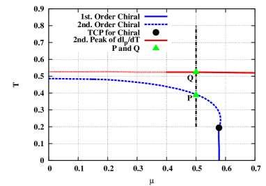
Figure 3: The phase boundary for the chiral transition with the second peak of $d\ell_{p}/dT$ at $\beta=4$ in the chiral limit. The “P” and “Q” correspond to those in Fig. 4 and in the upper panel of Fig. 6.

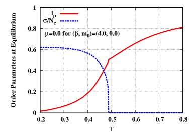
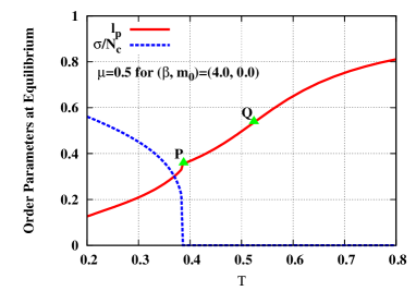
Figure 4: The $T$ dependence of the Polyakov loop and the chiral condensate for $\mu=0$ (upper) and $0.5$ (lower) at $(\beta,m_{0})=(4,0)$. In the lower panel, the “P” and “Q” correspond to those in Fig. 3 and the upper panel of Fig. 6.

We shall show the first P-SC-LQCD results including the “chiral and deconfinement” dynamics, “finite $\mu$ effects”, and “finite coupling effects” simultaneously. As shown in our recent work [32], the critical temperature at zero chemical potential becomes closer to the LQCD-MC results in the coupling region $\beta\lesssim 4$. Therefore, we focus our attention to the results at $\beta=4$. In the last part, we discuss the stability of our main conclusion for variations of $\beta$.

In Fig. 3, the phase diagram at $(\beta,m_{0})=(4,0)$ is shown in the lattice unit. We find the first- (solid blue) and second-order (dashed blue) chiral transition lines separated by the (tri-)critical point (CP) at $(\mu_{\mathrm{CP}},T_{\mathrm{CP}})=(0.58,0.19)$. The result is qualitatively consistent with the previous SC-LQCD with NLO effects [23]. In Fig. 4, we show the $T$ dependence of the chiral condensate $\sigma$ and the Polyakov loop $\ell_{p}$. The upper (lower) panel displays the results for $\mu=0~{}(0.5)$, i.e. on the $T$ axis (dash-dotted line) of the phase diagram in Fig. 3. We note $\mu=0.5<\mu_{\mathrm{CP}}$, and the following results would not be contaminated by the fluctuation around the CP.

We find two peaks in $d\ell_{p}/dT$. One peak appears at the chiral phase transition. For both $\mu=0$ and $0.5$ cases, the Polyakov loop $\ell_{p}$ shows a rapid increase at the chiral transition temperature ($\sigma\to 0$). The strong correlation of the Polyakov loop and $\sigma$ is found at any point on the chiral transition boundary. This correlation can be seen more clearly in the derivative $d\ell_{p}/dT$ as shown in Fig. 5. We find a sharp peak in the vicinity of the chiral phase transition, $T_{c,\mu=0}(\beta=4)\simeq 0.486$. The almost simultaneous observation of the chiral transition and the rapid change of $\ell_{p}$ would be consistent with the LQCD-MC results [1]. Via the $\sigma$-$\ell_{p}$ coupling in the Boltzmann factor terms in Eq. (11) and (12), the chiral transition would induce the rapid change of $\ell_{p}$. Thus we regard this peak as the chiral-induced peak.

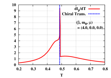
Figure 5: The $T$ dependence of $d\ell_{p}/dT$ in the chiral limit with zero chemical potential for $\beta=4$. The values are shown in the lattice unit $a=1$. The dashed blue line represents the critical temperature $T_{c,\mu=0}$ for the second-order chiral transition.

We also find the second peak above the chiral transition temperature in $d\ell_{p}/dT$. At $\mu=0$, a small enhancement is seen at around $T\simeq 0.52$. At finite $\mu$, the enhancement of $d\ell_{p}/dT$ at the second peak becomes significant. A similar double-peak structure has been reported in the model studies based on PNJL model [29]. In Fig. 6, we show $d\ell_{p}/dT$ along the line with $\mu=0.5$ (dash-dotted line in Fig. 3). In the chiral limit ($m_{0}\to 0$, upper panel), we find two peaks “P” and “Q”. Here, “P” and “Q” in Fig. 6 correspond to those in Figs. 3 and 4. The peak “P” locates at the chiral phase transition, and is clearly interpreted as the chiral-induced peak. As indicated by the red line in Fig. 3, the similar peak to “Q” is observed in the whole range of $\mu$. The strength of this peak becomes weaker for smaller $\mu$, which is expressed by the dotted line in Fig. 3.

The peak “Q” can be understood as a signal of the $Z_{N_{c}}$-induced crossover: $Z_{N_{c}}$ is the symmetry in the pure gluonic sector, and it becomes exact in the heavy quark mass limit. We also expect weak $\mu$ dependence of the $Z_{N_{c}}$ deconfinement transition, since $\mathcal{F}_{\mathrm{eff}}^{\mathrm{Pol}}$ does not directly depend on quark chemical potential $\mu$. In the middle and lower panels of Fig. 6, we show $d\ell_{p}/dT$ for $m_{0}=0.03$ and $m_{0}=1$, respectively. For $m_{0}=0.03$, we find two peaks. The temperature of the first peak “P” is slightly shifted upward and becomes closer to “Q” ($T_{\mathrm{Q}}$) with increasing $m_{0}$, while $T_{\mathrm{Q}}$ stays almost constant. For larger masses, $m_{0}>0.05$, the two peaks merges to a single peak, as shown in the lower panel of Fig. 6 for $m_{0}=1$. This single peak grows with increasing $m_{0}$, and its temperature is nearly $m_{0}$ independent, $T\sim 0.52$, which is close to $T_{\mathrm{Q}}$ at smaller quark masses. The $Z_{N_{c}}$-induced nature of “Q” and the merged single peak are confirmed by the weak dependence of $T_{\mathrm{Q}}$ on $\mu$ and $m_{0}$ as found in Figs. 3 and 6, respectively. It is interesting to find that the $Z_{N_{c}}$ nature survives in the chiral limit or small mass region, and can be observed as a peak in $d\ell_{p}/dT$.

There are several comments in order. (a) In cold dense matter in Fig. 3, the chiral symmetry is restored and Polyakov loop is suppressed. These features may be similar to those of quarkyonic matter [30]. (b) We find that $T_{\mathrm{Q}}$ is larger than the chiral phase transition temperature for small quark masses. In the chiral limit, the Polyakov loop $\ell_{p}$ decouples from the chiral dynamics at $T=T_{\mathrm{Q}}$ since $\sigma$-$\ell_{p}$ couplings in Eq. (15) vanish due to the exact chiral restoration $\sigma=0$. (c) We note that the chiral condensate decreasing rate, $-d\sigma/dT$, has a small peak at the $Z_{N_{c}}$-deconfinement crossover for $m_{0}=1$ as shown in the lower panel of Fig. 6. This peak is interpreted as a $Z_{N_{c}}$-induced peak. In this case, however, another peak which would stem from the chiral symmetry is completely overwhelmed due to the large quark mass, and the double-peak structure does not appear.

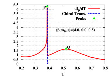
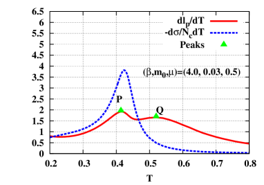
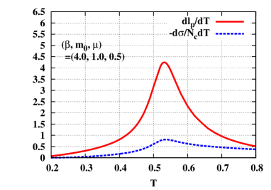
Figure 6: $T$ dependence of $d\ell_{p}/dT$ at $\mu=0.5$ for $\beta=4$ in the lattice unit. The current quark masses ($m_{0}$) are $0.0$ (upper), $0.03$ (middle), and $1$ (bottom). The dashed lines in the middle and lower panels represent $-(N_{c})^{-1}d\sigma/dT$.

Finally, we discuss the $\beta$ dependence of the two peak structure of $d\ell_{p}/dT$ at finite $\mu$. In Fig. 7, we show $d\ell_{p}/dT$ for several $\beta$ at $(m_{0},\mu)=(0.01,0.5)$. As indicated from this figure, the two peaks are found at least in the range $2\leq\beta\leq 6$. For each $\beta$, we define the pseudo-critical temperatures for the chiral-induced ($T_{c,\mu=0.5}^{(\chi)}(\beta)$) and $Z_{N_{c}}$-induced ($T_{c,\mu=0.5}^{(d)}(\beta)$) deconfinement crossovers as the first and second peaks of $d\ell_{p}/dT$, respectively. Both of them are decreasing functions of $\beta$. For $T_{c,\mu=0.5}^{(\chi)}(\beta)$, the current results are close to the pseudo-critical temperatures for the chiral phase transition in our previous works [23, 24]. This again indicates the chiral induced nature of the first peak “P”.

We find that the $\beta$ dependence of $T_{c,\mu=0.5}^{(d)}(\beta)$ is larger than that of $T_{c,\mu=0.5}^{(\chi)}(\beta)$, and the separation between two peaks tends to be narrower with increasing $\beta$ when chemical potential is fixed, $\mu=0.5$. Whereas the two peaks tend to be more separated for larger chemical potential for a fixed value of $\beta$. For example, two peak separation at $\mu=0.55$ becomes $1.4$ times larger than that at $\mu=0.5$ for $\beta=6$. This is because the chiral-induced transition temperature decreases in the large $\mu$ region of the $T-\mu$ plane, while there is no direct $\mu$ dependence in the $Z_{N_{c}}$ dynamics.

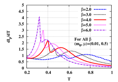
Figure 7: The $T$ dependence of $d\ell_{p}/dT$ for several $\beta$ at $(m_{0},\mu)=(0.01,0.5)$.

In summary, we have investigated the chiral and deconfinement crossovers at finite temperature $T$ and quark chemical potential $\mu$ based on the strong-coupling expansion in the lattice QCD with one species of staggered fermion. We have considered the leading and NLO effects in the strong-coupling expansion for fermionic sector, and the leading order Polyakov-loop effective action terms for the pure Yang-Mills sector. The $Z_{N_{c}}$ deconfinement dynamics has been incorporated to the Haar measure, where the Polyakov-loop is replaced with its constant mean-field value.

We have found double-peak structure in the Polyakov loop increasing rate $d\ell_{p}/dT$ as a function of $T$ for small quark masses and large $\mu$. The first peak is induced by the chiral transition. This is because the Polyakov loop $\ell_{p}$ becomes sensitive to the chiral dynamics through the coupling to the chiral condensate $\sigma$. For the larger quark mass $m_{0}$, the first peak is overwhelmed by the second peak, whose position is almost independent of $m_{0}$. This indicates that the second peak would attribute to the remnant $Z_{N_{c}}$ dynamics, which is less affected by $\mu$ than the chiral phase transition line due to the lack of a direct $\mu$ dependence in the Haar measure treatment for $Z_{N_{c}}$. Hence the double peaks, i.e.  the chiral and $Z_{N_{c}}$ induced peaks, come out in large $\mu$ region.

As future perspectives, we should evaluate the chiral and Polyakov-loop susceptibilities, next-to-next-to-leading order (NNLO) terms of strong coupling expansion for the chiral dynamics [24], higher order corrections of the Polyakov-loop effective action [6], and higher order terms of the $1/d$ expansion. The exact evaluation in each order of the strong-coupling expansion is also expected by the Monomer-Dimer-Polymer formulation [15, 19]. These corrections include couplings between the Polyakov loop and the chiral sector in the effective action level. Taking account of the resultant entanglement effects of the chiral and $Z_{N_{c}}$ dynamics, the appearance of chiral and $Z_{N_{c}}$ induced peaks must be investigated in future.

We would like to thank Maria Paola Lombardo, Lars Zeidlewicz, Philippe de Forcrand, Michael Fromm, and Kim Splittorff for fruitful discussions. We also thank Zoltan Fodor for useful comments for the critical temperature. This work was supported in part by Grants-in-Aid for Scientific Research from JSPS (No. 22-3314), the Yukawa International Program for Quark-hadron Sciences (YIPQS), and by Grants-in-Aid for the global COE program “The Next Generation of Physics, Spun from Universality and Emergence” from MEXT.

References

- [1] For recent results and reviews, see, S. Borsanyi, Z. Fodor, C. Hoelbling, S. D. Katz, S. Krieg, C. Ratti and K. K. Szabo [Wuppertal-Budapest Collaboration], JHEP 1009 (2010) 073.
- [2] K. G. Wilson, Phys. Rev. D 10, 2445 (1974).
- [3] M. Creutz, Phys. Rev. D 21, 2308 (1980); M. Creutz and K. J. M. Moriarty, Phys. Rev. D 26, 2166 (1982).
- [4] G. Münster, Nucl. Phys. B 180, 23 (1981).
- [5] J. Polonyi and K. Szlachanyi, Phys. Lett. B 110, 395 (1982); M. Gross, J. Bartholomew and D. Hochberg, “SU(N) Deconfinement Transition And The N State Clock Model”, Report No. EFI-83-35-CHICAGO, 1983.
- [6] J. Langelage and O. Philipsen, JHEP 1004 (2010) 055; JHEP 1001 (2010) 089; J. Langelage, G. Munster and O. Philipsen, JHEP 0807 (2008) 036.
- [7] The review of the pioneering works for the strong-coupling expansion is found in the text book, I. Montvay and G. Münster, “Quantum Fields on a Lattice,” Cambridge University Press, 1994.
- [8] N. Kawamoto and J. Smit, Nucl. Phys. B 192 (1981) 100.
- [9] H. Kluberg-Stern, A. Morel and B. Petersson, Nucl. Phys. B 215 (1983), 527.
- [10] H. Kluberg-Stern, A. Morel, O. Napoly and B. Petersson, Nucl. Phys. B 220 (1983) 447.
- [11] P. H. Damgaard, N. Kawamoto and K. Shigemoto, Nucl. Phys. B 264 (1986), 1.
- [12] P. H. Damgaard, D. Hochberg and N. Kawamoto, Phys. Lett. B 158, (1985) 239.
- [13] G. Fäldt and B. Petersson, Nucl. Phys. B 265, (1986) 197.
- [14] N. Bilic, F. Karsch and K. Redlich, Phys. Rev. D 45, (1992) 3228.
- [15] F. Karsch and K. H. Mutter, Nucl. Phys. B 313, (1989), 541.
- [16] Y. Nishida, K. Fukushima and T. Hatsuda, Phys. Rept. 398 (2004), 281; K. Fukushima, Prog. Theor. Phys. Suppl. 153 (2004), 204; Y. Nishida, Phys. Rev. D 69 (2004), 094501.
- [17] V. Azcoiti, G. Di Carlo, A. Galante and V. Laliena, J. High Energy Phys. 09 (2003), 014.
- [18] N. Kawamoto, K. Miura, A. Ohnishi and T. Ohnuma, Phys. Rev. D 75 (2007), 014502.
- [19] P. de Forcrand and M. Fromm, Phys. Rev. Lett. 104 (2010) 112005.
- [20] E. M. Ilgenfritz and J. Kripfganz, Z. Phys. C 29, (1985) 79; A. Gocksch and M. Ogilvie, Phys. Rev. D 31, (1985) 877.
- [21] K. Fukushima, Phys. Rev. D 68, (2003) 045004.
- [22] K. Fukushima, Phys. Lett. B 591 (2004), 277.
- [23] K. Miura, T. Z. Nakano, A. Ohnishi and N. Kawamoto, Phys. Rev. D 80 (2009) 074034; K. Miura, T. Z Nakano and A. Ohnishi, Prog. Theor. Phys. 122 (2009), 1045.
- [24] T. Z. Nakano, K. Miura and A. Ohnishi, Prog. Theor. Phys. 123 (2010) 825.
- [25] K. Miura, T. Z. Nakano, A. Ohnishi and N. Kawamoto, PoS LATTICE2010 (2010) 202.
- [26] K. Fukushima, Phys. Lett. B 695, 387 (2011).
- [27] T. K. Herbst, J. M. Pawlowski and B. J. Schaefer, Phys. Lett. B 696 (2011) 58.
- [28] K. Fukushima, Phys. Rev. D 77, (2008) 114028.
- [29] T. Kahara and K. Tuominen, Phys. Rev. D 82 (2010) 114026; Phys. Rev. D 78 (2008) 034015; Phys. Rev. D 80 (2009) 114022.
- [30] L. McLerran, K. Redlich and C. Sasaki, Nucl. Phys. A 824 (2009) 86.
- [31] Y. Sakai, T. Sasaki, H. Kouno and M. Yahiro, Phys. Rev. D 82 (2010) 076003.
- [32] T. Z. Nakano, K. Miura and A. Ohnishi, Phys. Rev. D 83 (2011) 016014; T. Z. Nakano, K. Miura and A. Ohnishi, PoS LATTICE2010 (2010) 205.
- [33] M. F. L. Golterman and J. Smit, Nucl. Phys. B 245, (1984) 61; M. F. L. Golterman and J. Smit, Nucl. Phys. B 255, (1985) 328;
- [34] For recent reviews for numerical aspects of staggered flavors, see the first half of, A. S. Kronfeld, Proc. Sci. LAT2007, (2007) 016; S. R. Sharpe, Proc. Sci. LAT2006, (2006) 022.
- [35] J. B. Kogut, M. Snow and M. Stone, Nucl. Phys. B 200, 211 (1982).
- [36] L. McLerran and R. D. Pisarski, Nucl. Phys. A 796 (2007), 83; Y. Hidaka, L. D. McLerran and R. D. Pisarski, Nucl. Phys. A 808 (2008), 117.