On a Hamiltonian version of a 3D Lotka-Volterra system

Abstract

In this paper we present some relevant dynamical properties of a 3D Lotka-Volterra system from the Poisson dynamics point of view.

AMS 2000: 70H05; 37J25; 37J35.

Keywords: Hamiltonian dynamics, Lotka-Volterra system, stability of equilibria, Poincaré compactification, energy-Casimir mapping.

1 Introduction

The Lotka-Volterra system has been widely investigated in the last years. This system, studied by May and Leonard [8], models the evolution of competition between three species. Among the studied topics related with the Lotka-Volterra system, we recall a few of them together with a partial list of references, namely: integrals and invariant manifolds ([2], [4]), stability ([7], [2]), analytic behavior [3], nonlinear analysis [8], and many others.

In this paper we consider a special case of the Lotka-Volterra system, recently introduced in [4]. We write the system as a Hamiltonian system of Poisson type in order to analyze the system from the Poisson dynamics point of view. More exactly, in the second section of this paper, we prepare the framework of our study by writing the Lotka-Volterra system as a Hamilton-Poisson system, and also find a $SL(2,\mathbb{R})$ parameterized family of Hamilton-Poisson realizations. As consequence of the Hamiltonian setting we obtain two new first integrals of the Lotka-Volterra system that generates the first integrals of this system found in [4]. In the third section of the paper we determine the equilibria of the Lotka-Volterra system and then analyze their Lyapunov stability. The fourth section is dedicated to the study of the Poincaré compactification of the Lotka-Volterra system. More exactly, we integrate explicitly the Poincaré compactification of the Lotka-Volterra system. In the fifth section of the article we present some convexity properties of the image of the energy-Casimir mapping and define some naturally associated semialgebraic splittings of the image. More precisely, we discuss the relation between the image through the energy-Casimir mapping of the families of equilibria of the Lotka-Volterra system and the canonical Whitney stratifications of the semialgebraic splittings of the image of the energy-Casimir mapping. In the sixth part of the paper we give a topological classification of the fibers of the energy-Casimir mapping, classification that follows naturally from the stratifications introduced in the above section. Note that in our approach we consider fibers over the regular and also over the singular values of the energy-Casimir mapping. In the last part of the article we give two Lax formulations of the system. For details on Poisson geometry and Hamiltonian dynamics see e.g. [6], [9], [1], [11].

2 Hamilton-Poisson realizations of a 3D Lotka-Volterra system

The Lotka-Volterra system we consider for our study, is governed by the equations:

$$\left\{\begin{array}[]{l}\dot{x}=-x(x-y-z)\\ \dot{y}=-y(-x+y-z)\\ \dot{z}=-z(-x-y+z).\\ \end{array}\right.$$ (2.1)

Note that the above system is the Lotka-Volterra system studied in [4] in the case $a=b=-1$.

In [4] it is shown that this system admits the following polynomial conservation laws:

$$f(x,y,z)=xyz(x-y)(x-z)(y-z),$$

$$g(x,y,z)=x^{2}y^{2}-x^{2}yz-xy^{2}z+x^{2}z^{2}-xyz^{2}+y^{2}z^{2}.$$

Using Hamiltonian setting of the problem, we provide two degree-two polynomial conservation laws of the system (2.1) which generates $f$ and $g$. These conservation laws will be represented by the Hamiltonian and respectively a Casimir function of the Poisson configuration manifold of the system (2.1).

As the purpose of this paper is to study the above system from the Poisson dynamics point of view, the first step in this approach is to give a Hamilton-Poisson realization of the system.

Theorem 2.1

The dynamics (2.1) has the following Hamilton-Poisson realization:

$$({\mathbb{R}}^{3},\Pi_{C},H)$$ (2.2)

where,

$$\Pi_{C}(x,y,z)=\left[{\begin{array}[]{*{20}c}0&y&{x-z}\\ -y&0&{-y}\\ {-x+z}&{y}&0\\ \end{array}}\right]$$

is the Poisson structure generated by the smooth function $C(x,y,z):=-xy+yz$, and the Hamiltonian $H\in C^{\infty}({\mathbb{R}}^{3},{\mathbb{R}})$ is given by $H(x,y,z):=xy-xz$.

Note that, by Poisson structure generated by the smooth function $C$, we mean the Poisson structure generated by the Poisson bracket $\{f,g\}:=\nabla C\cdot(\nabla f\times\nabla g)$, for any smooth functions $f,g\in C^{\infty}({\mathbb{R}}^{3},{\mathbb{R}})$.

Proof. Indeed, we have successively:

$$\Pi_{C}(x,y,z)\cdot\nabla H(x,y,z)=\left[{\begin{array}[]{*{20}c}0&{y}&{x-z}\\ {-y}&0&{-y}\\ {-x+z}&{y}&0\\ \end{array}}\right]\cdot\left[{\begin{array}[]{*{20}c}{y-z}\\ {x}\\ {-x}\\ \end{array}}\right]=\left[{\begin{array}[]{*{20}l}{-x(x-y-z)}\\ {-y(-x+y-z)}\\ {-z(-x-y+z)}\\ \end{array}}\right]=\left[{\begin{array}[]{*{20}r}{\dot{x}}\\ {\dot{y}}\\ {\dot{z}}\\ \end{array}}\right],$$

as required.   

Remark 2.2

Since the signature of the quadratic form generated by $C(x,y,z)=-xy+yz$ is $(-1,0,+1)$, the triple $(\mathbb{R}^{3},\Pi_{C},H)$ it is isomorphic with a Lie-Poisson realization of the Lotka-Volterra system (2.1) on the dual of the semidirect product between the Lie algebra $\mathfrak{so}(1,1)$ and $\mathbb{R}^{2}$.

Remark 2.3

By definition we have that the center of the Poisson algebra $C^{\infty}(\mathbb{R}^{3},{\mathbb{R}})$ is generated by the Casimir invariant $C(x,y,z)=-xy+yz$.

Remark 2.4

The conservation laws $f$ and $g$ found in [4], can be written in terms of the Casimir $C$ and respectively the Hamiltonian $H$ as follows:

$$f=CH(C+H),$$

$$g=\dfrac{1}{2}\left[C^{2}+H^{2}+(C+H)^{2}\right].$$

Next proposition gives others Hamilton-Poisson realizations of the Lotka-Volterra system (2.1).

Proposition 2.5

The dynamics (2.1) admits a family of Hamilton-Poisson realizations parameterized by the group $SL(2,{\mathbb{R}})$. More exactly, $({\mathbb{R}}^{3},\{\cdot,\cdot\}_{a,b},H_{c,d})$ is a Hamilton-Poisson realization of the dynamics (2.1) where the bracket $\{\cdot,\cdot\}_{a,b}$ is defined by

$$\{f,g\}_{a,b}:=\nabla C_{a,b}\cdot(\nabla f\times\nabla g),$$

for any $f,g\in C^{\infty}({\mathbb{R}}^{3},{\mathbb{R}})$, and the functions $C_{a,b}$ and $H_{c,d}$ are given by:

$$C_{a,b}(x,y,z)=(-a+b)xy+ayz-bxz,$$

$$H_{c,d}(x,y,z)=(-c+d)xy+cyz-dxz,$$

respectively, the matrix of coefficients $a,b,c,d$ is $\left[{\begin{array}[]{*{20}c}a&b\\ c&d\\ \end{array}}\right]\in SL(2,{\mathbb{R}}).$

Proof. The conclusion follows directly taking into account that the matrix formulation of the Poisson bracket $\{\cdot,\cdot\}_{a,b}$ is given in coordinates by:

$$\Pi_{a,b}(x,y,z)=\left[{\begin{array}[]{*{20}c}0&{-bx+ay}&{(a-b)x-az}\\ {bx-ay}&0&{(-a+b)y-bz}\\ {(-a+b)x+az}&{(a-b)y+bz}&0\end{array}}\right].$$

 

3 Stability of equilibria

In this short section we analyze the stability properties of the equilibrium states of the Lotka-Volterra system (2.1).

Remark 3.1

The equilibrium states of the system (2.1) are given as the union of the following three families:

$${\mathcal{E}}_{1}:=\{(0,M,M):M\in{\mathbb{R}}\},$$

$${\mathcal{E}}_{2}:=\{(M,0,M):M\in{\mathbb{R}}\},$$

$${\mathcal{E}}_{3}:=\{(M,M,0):M\in{\mathbb{R}}\}.$$

Figure 1 presents the above defined families of equilibrium states of the Lotka-Volterra system.

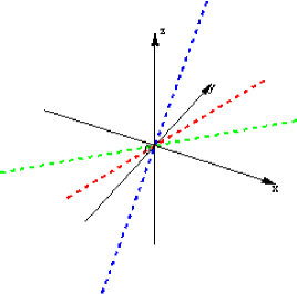
Figure 1: Equilibria of the Lotka-Volterra system (2.1).

In the following theorem we describe the stability properties of the equilibrium states of the system (2.1).

Theorem 3.2

All the equilibrium states of the Lotka-Volterra system (2.1) are unstable.

Proof. The conclusion follows from the fact that the characteristic polynomial associated with the linear part of the system evaluated at an arbitrary equilibrium state, is the same for any of the families $\mathcal{E}_{1},\mathcal{E}_{2},\mathcal{E}_{3}$, and is given by:

$$p(\lambda)=(2M-\lambda)\lambda(2M+\lambda).$$

For $M=0$, we get the origin $(0,0,0)$ which is also unstable since in any arbitrary small open neighborhood around, there exists unstable equilibrium states.   

4 The behavior on the sphere at infinity

In this section we integrate explicitly the Poincaré compactification of the Lotka-Volterra system, and consequently the Lotka-Volterra system (2.1) (on the sphere) at infinity. Recall that using the Poincaré compactification of ${\mathbb{R}}^{3}$, the infinity of ${\mathbb{R}}^{3}$ is represented by the sphere $\mathbb{S}^{2}$ - the equator of the unit sphere $\mathbb{S}^{3}$ in ${\mathbb{R}}^{4}$. For details regarding the Poincaré compactification of polynomial vector fields in ${\mathbb{R}}^{3}$ see [5].

Fixing the notations in accordance with the results stated in [5] we write the Lotka-Volterra system (2.1) as

$$\left\{\begin{array}[]{l}\dot{x}=P^{1}(x,y,z)\\ \dot{y}=P^{2}(x,y,z)\\ \dot{z}=P^{3}(x,y,z),\\ \end{array}\right.$$

with $P^{1}(x,y,z)=-x(x-y-z)$, $P^{2}(x,y,z)=-y(-x+y-z)$, $P^{3}(x,y,z)=-z(-x-y+z)$.

Let us now study the Poincaré compactification of the Lotka-Volterra system in the local charts $U_{i}$ and $V_{i}$, $i\in\{1,2,3\}$, of the manifold $\mathbb{S}^{3}$.

The Poincaré compactification ($p(X)$ in the notations from [5]) of the Lotka-Volterra system (2.1) is the same for each of the local charts $U_{1}$, $U_{2}$ and respectively $U_{3}$ and is given in the corresponding local coordinates by

$$\left\{\begin{array}[]{l}\dot{z}_{1}=2z_{1}(1-z_{1})\\ \dot{z}_{2}=2z_{2}(1-z_{2})\\ \dot{z}_{3}=-z_{3}(z_{1}+z_{2}+1).\\ \end{array}\right.$$ (4.1)

Regarding the Poincaré compactification of the Lotka-Volterra system in the local charts $V_{1}$, $V_{2}$ and respectively $V_{3}$, as a property of the compactification procedure, the compactified vector field $p(X)$ in the local chart $V_{i}$ coincides with the vector field $p(X)$ in $U_{i}$ multiplied by the factor $-1$, for each $i\in\{1,2,3\}$. Hence, for each $i\in\{1,2,3\}$, the flow of the system (4.1) on the local chart $V_{i}$ is the same as the flow on the local chart $U_{i}$ reversing the time.

The system (4.1) is integrable with the solution given by

$$\left\{\begin{array}[]{l}z_{1}(t)=\dfrac{e^{2t}}{e^{2t}+e^{k_{1}}}\\ z_{2}(t)=\dfrac{e^{2t}}{e^{2t}+e^{k_{2}}}\\ z_{3}(t)=\dfrac{e^{t}k_{3}}{\sqrt{e^{2t}+e^{k_{1}}}\sqrt{e^{2t}+e^{k_{2}}}},\\ \end{array}\right.$$

where $k_{1},k_{2},k_{3}$ are arbitrary real constants.

To analyze the Lotka-Volterra system on the sphere $\mathbb{S}^{2}$ at infinity, note that the points on the sphere at infinity are characterized by $z_{3}=0$. As the plane $z_{1}z_{2}$ is invariant under the flow of the system (4.1), the compactified Lotka-Volterra system on the local charts $U_{i}$ ($i\in\{1,2,3\}$) on the infinity sphere reduces to

$$\left\{\begin{array}[]{l}\dot{z}_{1}=2z_{1}(1-z_{1})\\ \dot{z}_{2}=2z_{2}(1-z_{2}).\\ \end{array}\right.$$ (4.2)

The system (4.2) is integrable and the solution is given by

$$\left\{\begin{array}[]{l}z_{1}(t)=\dfrac{e^{2t}}{e^{2t}+e^{k_{1}}}\\ z_{2}(t)=\dfrac{e^{2t}}{e^{2t}+e^{k_{2}}},\\ \end{array}\right.$$

where $k_{1},k_{2}$ are arbitrary real constants.

Consequently, the phase portrait on the local charts $U_{i}$ ($i\in\{1,2,3\}$) on the infinity sphere is given in Figure 2.

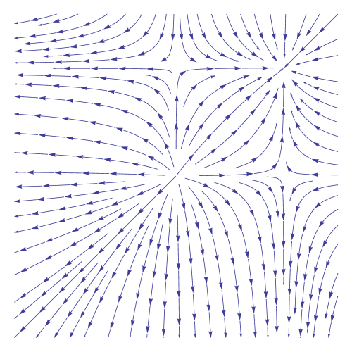
Figure 2: Phase portrait of the system (4.2).

5 The image of the energy-Casimir mapping

The aim of this section is to study the image of the energy-Casimir mapping $Im(\mathcal{E}C)$, associated with the Hamilton-Poisson realization (2.2) of the Lotka-Volterra system (2.1).

We consider convexity properties of the image of $\mathcal{E}C$, as well as a semialgebraic splitting of the image that agree with the topology of the symplectic leaves of the Poisson manifold $({\mathbb{R}}^{3},\Pi_{C})$. Recall that by a semialgebraic splitting, we mean a splitting consisting of semialgebraic manifolds, namely manifolds that are described in coordinates by a set of polynomial inequalities and equalities. For details on semialgebraic manifolds and their geometry see e.g. [10].

All these will be used later on, in order to obtain a topological classification of the orbits of (2.1).

Recall first that the energy-Casimir mapping, ${\mathcal{E}C}\in C^{\infty}({\mathbb{R}}^{3},{\mathbb{R}}^{2})$ is given by:

$${\mathcal{E}C}(x,y,z)=(H(x,y,z),C(x,y,z)),\ (x,y,z)\in{\mathbb{R}}^{3}$$

where $H,C\in C^{\infty}({\mathbb{R}}^{3},{\mathbb{R}})$ are the Hamiltonian of the system (2.1), and respectively the Casimir of the Poisson manifold $({\mathbb{R}}^{3},\Pi_{C})$, both of them as considered in Theorem 2.1.

Next proposition explicitly gives the semialgebraic splitting of the image of the energy-Casimir map ${\mathcal{E}C}$.

Proposition 5.1

The image of the energy-Casimir map - ${\mathbb{R}}^{2}$ - admits the following splitting:

$Im(\mathcal{E}C)=S^{c>0}\cup S^{c=0}\cup S^{c<0}$, where the subsets $S^{c>0}$, $S^{c=0}$, $S^{c<0}\subset{\mathbb{R}}^{2}$ are splitting further on a union of semialgebraic manifolds, as follows:

$$S^{c>0} =\{(h,c)\in{\mathbb{R}}^{2}:h<0;c>0\}\cup\{(h,c)\in{\mathbb{R}}^{2}:h=0;c>0\}$$

$$\cup\{(h,c)\in{\mathbb{R}}^{2}:h>0;c>0\},$$

$$S^{c=0} =\{(h,c)\in{\mathbb{R}}^{2}:h<0;c=0\}\cup\{(h,c)\in{\mathbb{R}}^{2}:h=c=0\}$$

$$\cup\{(h,c)\in{\mathbb{R}}^{2}:h>0;c=0\},$$

$$S^{c<0} =\{(h,c)\in{\mathbb{R}}^{2}:c<\min\{-h,0\}\}\cup\{(h,c)\in{\mathbb{R}}^{2}:c<0;c=-h\}$$

$$\cup\{(h,c)\in{\mathbb{R}}^{2}:-h<c<0\}.$$

Proof. The conclusion follows directly by simple algebraic computation using the definition of the energy-Casimir mapping.   

Remark 5.2

The superscripts used to denote the sets $S$, are in agreement with the topology of the symplectic leaves of the Poisson manifold $({\mathbb{R}}^{3},\Pi_{C})$, namely:

• For $c\neq 0$,

  $${\Gamma}_{c}=\{(x,y,z)\in{\mathbb{R}}^{3}:y(z-x)=c\}$$

  is a hyperbolic cylinder.

• For $c=0$,

  $${\Gamma}_{c}=\{(x,y,z)\in{\mathbb{R}}^{3}:y(z-x)=c\}$$

  is a union of two intersecting planes.

The connection between the semialgebraic splittings of the image $Im({\mathcal{E}C})$ given by Proposition 5.1, and the equilibrium states of the Lotka-Volterra system, is given in the following remark.

Remark 5.3

The semialgebraic splitting of the sets $S$ is described in terms of the image of equilibria of the Lotka-Volterra system through the map $\mathcal{E}C$ as follows:

• $$\ S^{c>0} =\Sigma_{1}^{\leftarrow}\cup Im(\left.{\mathcal{E}C}\right|_{{\mathcal{E}}_{1}^{\star}})\cup\Sigma_{1}^{\rightarrow},\ where\ {\mathcal{E}}_{1}^{\star}={\mathcal{E}}_{1}\setminus\{(0,0,0)\},$$

  $$\Sigma_{1}^{\leftarrow} =\{(h,c)\in{\mathbb{R}}^{2}:h<0;c>0\},\ \Sigma_{1}^{\rightarrow}=\{(h,c)\in{\mathbb{R}}^{2}:h>0;c>0\}.$$

• $$\ S^{c=0} =Im(\left.{\mathcal{E}C}\right|_{{\mathcal{E}}_{2}^{\star}})\cup\Sigma_{0}\cap\Sigma_{0}^{\rightarrow},\ where\ {\mathcal{E}}_{2}^{\star}={\mathcal{E}}_{2}\setminus\{(0,0,0)\},$$

  $$\Sigma_{0} =\{(0,0,0)\},\ \Sigma_{0}^{\rightarrow}=\{(h,c)\in{\mathbb{R}}^{2}:h>0;c=0\}.$$

• $$\ S^{c<0} =\Sigma_{3}^{\leftarrow}\cup Im(\left.{\mathcal{E}C}\right|_{{\mathcal{E}}_{3}^{\star}})\cup\Sigma_{3}^{\rightarrow},\ where\ {\mathcal{E}}_{3}^{\star}={\mathcal{E}}_{3}\setminus\{(0,0,0)\},$$

  $$\Sigma_{3}^{\leftarrow} =\{(h,c)\in{\mathbb{R}}^{2}:c<\min\{-h,0\}\},\ \Sigma_{3}^{\rightarrow}=\{(h,c)\in{\mathbb{R}}^{2}:-h<c<0\}.$$

All the stratification results can be gathered as shown in Figure 3. Note that for simplicity we adopted the notation $Im(\left.{\mathcal{E}C}\right|_{{\mathcal{E}}})\mathop{=}\limits^{not}:\Sigma$.

$Im({\mathcal{E}C})$
$S^{c>0}$	$S^{c=0}$
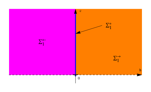
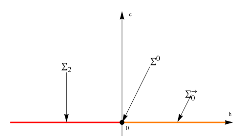
$S_{0}^{c<0}$
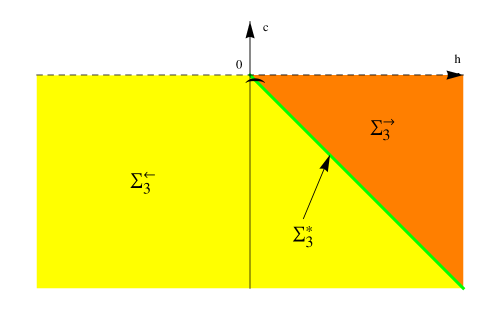
$S_{0}^{c>0}\cup S_{0}^{c=0}\cup S_{0}^{c<0}$

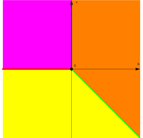
Figure 3: Semialgebraic splitting of $Im({\mathcal{E}C})$.

Remark 5.4

As a convex set, the image of the energy-Casimir map is convexly generated by the images of the equilibrium states of the Lotka-Volterra system (2.1), namely:

$$Im({\mathcal{E}C})=\overline{\rm co}\{Im(\left.{\mathcal{E}C}\right|_{{\mathcal{E}}_{1}}),Im(\left.{\mathcal{E}C}\right|_{{\mathcal{E}}_{2}}),Im(\left.{\mathcal{E}C}\right|_{{\mathcal{E}}_{3}})\}.$$

6 The topology of the fibers of the energy-Casimir mapping

In this section we describe the topology of the fibers of $\mathcal{E}C$, considering for our study fibers over regular values of $\mathcal{E}C$ as well as fibers over the singular values. It will remain an open question how these fibers fit all together in a more abstract fashion, such as bundle structures in the symplectic Arnold-Liouville integrable regular case.

Proposition 6.1

According to the stratifications from the previous section, the topology of the fibers of $\mathcal{E}C$ can be described as in Tables 1, 2, 3:

$S^{c>0}$
$A\subseteq S^{c>0}$	$\Sigma_{1}^{\leftarrow}$	$\Sigma_{1}^{*}$	$\Sigma_{1}^{\rightarrow}$
${\cal F}_{(h,c)}\subseteq{\mathbb{R}}^{3}$
$(h,c)\in A$	$\mathop{\coprod}\limits_{i=1}^{4}({\mathbb{R}}\times\{i\})$	$\mathop{\coprod}\limits_{i=1}^{8}({\mathbb{R}}\times\{i\})\mathop{\coprod}\{pt\}\mathop{\coprod}\{pt^{\prime}\}$	$\mathop{\coprod}\limits_{i=1}^{4}({\mathbb{R}}\times\{i\})$
Dynamical	union of	union of 8	union of
description	4 orbits	orbits and two	4 orbits
		equilibrium points

Table 1: Fibers classification corresponding to $S^{c>0}$.

$S^{c=0}$
$A\subseteq S^{c=0}$	$\Sigma_{2}$	$\Sigma^{0}$	$\Sigma_{0}^{\rightarrow}$
${\cal F}_{(h,c)}\subseteq{\mathbb{R}}^{3}$
$(h,c)\in A$	$\coprod\limits_{i=1}^{8}({\mathbb{R}}\times\{i\})\coprod\{pt\}\coprod\{pt^{\prime}\}$	$\coprod\limits_{i=1}^{8}({\mathbb{R}}\times\{i\})\coprod\{pt\}$	$\coprod\limits_{i=1}^{4}({\mathbb{R}}\times\{i\})$
Dynamical	union of 8	union of 8	union of
description	orbits and two	orbits and one	4 orbits
	equilibrium points	equilibrium point

Table 2: Fibers classification corresponding to $S^{c=0}$.

$S^{c<0}$
$A\subseteq S^{c<0}$	$\Sigma_{3}^{\leftarrow}$	$\Sigma_{3}^{*}$	$\Sigma_{3}^{\rightarrow}$
${\cal F}_{(h,c)}\subseteq{\mathbb{R}}^{3}$
$(h,c)\in A$	$\mathop{\coprod}\limits_{i=1}^{4}({\mathbb{R}}\times\{i\})$	$\mathop{\coprod}\limits_{i=1}^{8}({\mathbb{R}}\times\{i\})\mathop{\coprod}\{pt\}\mathop{\coprod}\{pt^{\prime}\}$	$\mathop{\coprod}\limits_{i=1}^{4}({\mathbb{R}}\times\{i\})$
Dynamical	union of	union of 8	union of
description	4 orbits	orbits and two	4 orbits
		equilibrium points

Table 3: Fibers classification corresponding to $S^{c<0}$.

Proof. The conclusion follows by simple computations according to the topology of the solution set of the system:

$$\left\{\begin{array}[]{l}H(x,y,z)=h\\ C(x,y,z)=c\\ \end{array}\right.$$

where $(h,c)$ belongs to the semialgebraic manifolds introduced in the above section.   

A presentation that puts together the topological classification of the fibers of $\mathcal{E}C$ and the topological classification of the symplectic leaves of the Poisson manifold $({\mathbb{R}}^{3},\Pi_{C})$, is given in Figure 4.

${\mathcal{E}C}^{-1}({\mathbb{R}}^{2})={\mathcal{E}C}^{-1}(Im({\mathcal{E}C}))$
${\mathcal{E}C}^{-1}(S^{c<0})$	${\mathcal{E}C}^{-1}(S^{c=0})$
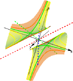
${\mathcal{E}C}^{-1}(S^{c>0})$
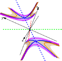
${\mathcal{E}C}^{-1}({\mathbb{R}}^{2})={\mathcal{E}C}^{-1}(S^{c<0})\cup{\mathcal{E}C}^{-1}(S^{c=0})\cup{\mathcal{E}C}^{-1}(S^{c>0})$

Figure 4: Phase portrait splitting.

7 Lax Formulation

In this section we present a Lax formulation of the Lotka-Volterra system (2.1).

Let us first note that as the system (2.1) restricted to a regular symplectic leaf, give rise to a sypmlectic Hamiltonian system that is completely integrable in the sense of Liouville and consequently it has a Lax formulation.

Is a natural question to ask if the unrestricted system admit a Lax formulation. The answer is positive and is given by the following proposition:

Proposition 7.1

The Lotka-Volterra system (2.1) can be written in the Lax form $\dot{L}=[L,B]$, where the matrices $L$ and respectively $B$ are given by:

$$L=\left[{\begin{array}[]{*{20}c}0&{x-y}&{z}\\ {-x+y}&0&{i(x+y-z)}\\ {-z}&{-i(x+y-z)}&0\\ \end{array}}\right],\ B=\left[{\begin{array}[]{*{20}c}0&{iz}&{i(x-y)}\\ {-iz}&0&0\\ {-i(x-y)}&0&0\\ \end{array}}\right].$$

R.M. Tudoran
The West University of Timişoara
Faculty of Mathematics and C.S., Department of Mathematics,
B-dl. Vasile Parvan, No. 4,
300223-Timişoara, Romania.
E-mail: tudoran@math.uvt.ro
Supported by CNCSIS-UEFISCDI, project number PN II-IDEI code 1081/2008 No. 550/2009.

A. Gîrban
”Politehnica” University of Timişoara
Department of Mathematics,
Piaţa Victoriei nr. 2,
300006-Timişoara, România.
E-mail: anania.girban@gmail.com

References

- [1] R.H. Cushman and L. Bates, Global aspects of classical integrable systems (1977), Basel: Birkhauser.
- [2] P.G.L. Leach and J. Miritzis, Competing species: integrability and stability, J. Nonlinear Math. Phys., 11 (2004), 123–133.
- [3] P.G.L. Leach and J. Miritzis, Analytic behavior of competition among three species, J. Nonlinear Math. Phys., 13 (2006), 535–548.
- [4] J. Llibre and C. Valls, Polynomial, rational and analytic first integrals for a family of 3-dimensional Lotka-Volterra systems, Z. Angew. Math. Phys., (2011), DOI 10.1007/s00033-011-0119-2.
- [5] C.A. Buzzi, J. Llibre and J.C. Medrado, Periodic orbits for a class of reversible quadratic vector field on , J. Math. Anal. Appl., 335 (2007), 1335–1346.
- [6] J.E. Marsden, Lectures on mechanics, London Mathematical Society Lecture Notes Series, vol. 174, Cambridge University Press.
- [7] R.M. May, Stability and Complexity in Model Ecosystems(1974), Second Edition, Princeton University Press, Princeton.
- [8] R.M. May and W.J. Leonard, Nonlinear aspects of competition between three species, SIAM J. Appl. Math., 29 (1975), 243–256.
- [9] J.E. Marsden and T.S. Ratiu, Introduction to mechanics and symmetry, Texts in Applied Mathematics, vol. 17, second edition, second printing, Springer, Berlin.
- [10] M.J. Pflaum, Analytic and geometric study of stratified spaces (2001), Lecture Notes in Mathematics, vol. 510, Springer, Berlin.
- [11] T.S. Ratiu, R.M. Tudoran, L. Sbano, E. Sousa Dias and G. Terra, Geometric Mechanics and Symmetry: the Peyresq Lectures; Chapter II: A Crash Course in Geometric Mechanics, pp. 23–156, London Mathematical Society Lecture Notes Series, vol. 306 (2005), Cambridge University Press.