Collective Uncertainty Entanglement Test

Abstract

For a given pure state of a composite quantum system we analyze the product of its projections onto a set of locally orthogonal separable pure states. We derive a bound for this product analogous to the entropic uncertainty relations. For bipartite systems the bound is saturated for maximally entangled states and it allows us to construct a family of entanglement measures, we shall call collectibility. As these quantities are experimentally accessible, the approach advocated contributes to the task of experimental quantification of quantum entanglement, while for a three–qubit system it is capable to identify the genuine three-party entanglement.

The phenomenon of quantum entanglement – non–classical correlations between individual subsystems – is a subject of an intense research interest MCKB05 ; BZ06 ; HHHH09 . Several criteria of detecting entanglement are known BZ06 ; HHHH09 , and some of them can be implemented experimentally (see PR_Guhne for the review of specific experimental schemes). In particular the issue of qualitative entanglement detection is quite well established including entanglement witnesses method (see HHHH09 ) and local uncertainty relations Uncertainty . On the other hand, although various measures of quantum entanglement are analyzed PV07 ; HHHH09 , in general they are more difficult to be quantitatively measured in a physical experiment. To estimate experimentally the degree of entanglement of a given quantum state one usually relies SM+08 on quantum tomography or analogous techniques.

The idea of entanglement detection and estimation without prior tomography HE02 ; PH03 involves the collective measurement of two (or more) copies of the state as demonstrated in BCEHAS05 . Consequently recent attempts towards experimental quantification of entanglement are based on finding collectively measurable quantities which bound known entanglement measures from below and are experimentally accessible MKB05a ; WRDMB06 (for review see AL09 ).

The main aim of this work is to construct a family of indicators, designed to quantify the entanglement of a pure state of an arbitrary composite system, which can be measured in a coincidence experiment without attempting for a complete reconstruction of the quantum state.

Our approach, which leads to simple collective entanglement test, is inspired by the entropic uncertainty relations which are satisfied by any pure state. For instance, the sum of the Shannon entropies of the expansion coefficients of a given pure state $|\psi\rangle\in{\cal H}_{N}$ expanded in two mutually unbiased bases is bounded from below by $\ln N$ MU88 . This observation suggests to quantify the pure states entanglement by a function of the projections of the analyzed state $|\Psi\rangle$ of a composite system onto mutually orthogonal separable pure states.

The method we propose can be formulated in a rather general case of a normalized pure state, $\langle\Psi|\Psi\rangle=1$, of a composite system consisting of $K$ subsystems. For simplicity we shall assume here that all their dimensions are equal, so we consider an element of a K-partite Hilbert space $\mathcal{H}=\mathcal{H}^{A}\otimes{H}^{B}\ldots\otimes\mathcal{H}^{K}$, where $\dim\left(\mathcal{H}^{A}\right)=\ldots=\dim\left(\mathcal{H}^{K}\right)=N$. Let us select a set of $N$ separable pure states of a $K$–quNit system, $|\chi_{j}^{sep}\rangle=|a_{j}^{A}\rangle\otimes\ldots\otimes\left|a_{j}^{K}\right\rangle$. where $|a_{j}^{I}\rangle\in\mathcal{H}^{I}$ with $j=1,\dots,N$ and $I=A,\dots,K$. The key assumption is that all local states are mutually orthogonal, so that

$$\left|a_{1}^{I}\right\rangle,\ldots,\left|a_{N}^{I}\right\rangle\in\mathcal{H}^{I},\qquad\left.\left\langle a_{j}^{I}\right|a_{k}^{I}\right\rangle=\delta_{jk}.$$ (1)

Entanglement detection —

In order to construct measurable indicators of quantum entanglement and find practical entanglement criteria valid for any analyzed state $|\Psi\rangle$ we define now the following quantity

$$Y^{max}\left[\left|\Psi\right\rangle\right]=\max_{\left|\chi^{sep}\right\rangle}\prod_{j=1}^{N}\left|\!\left.\left\langle\Psi\right|\chi_{j}^{sep}\right\rangle\right|^{2}.$$ (2)

This product of the projections of the state onto the set of $N$ separable states, optimized over all possible sets of mutually locally orthogonal states, $|\chi^{sep}\rangle=\{|\chi_{1}^{sep}\rangle,\ldots,|\chi_{N}^{sep}\rangle\}$, will be called maximal collectibility.

Note the difference with respect to the geometric measure of entanglement WG03 , to define which one takes the maximum over a single separable state, $|\chi_{1}^{sep}\rangle$. In this case this maximum, denoted in WG03 by $\Lambda^{2}_{max}$, is equal to unity if the analyzed state $|\Psi\rangle$ is separable and it is smaller for any entangled state, so to define the geometric measure of entanglement one takes $1-\Lambda^{2}_{max}$. In contrast, taking in (2) the maximum of the product of the projections of $|\Psi\rangle$ onto $N\geq 2$ separable states $|\chi_{j}^{sep}\rangle$ we face an inverse situation: we show below that $Y^{max}$ is the largest for maximally entangled states, so this quantity can serve directly as a quantificator of entanglement.

To this end we shall start with a variational equation

$$\frac{\delta}{\delta\left|\Psi\right\rangle}\left(\prod_{j=1}^{N}\left|\!\left.\left\langle\Psi\right|\chi_{j}^{sep}\right\rangle\right|^{2}-\lambda\!\left.\left\langle\Psi\right|\Psi\right\rangle\right)=0,$$ (3)

where $\lambda$ plays the role of a Lagrange multiplier associated with the normalization constraint. This idea was developed by Deutsch in order to obtain the entropic uncertainty relation Deutsch . Equation (3) implies

$$\prod_{j=1}^{N}\left|\!\left.\left\langle\Psi\right|\chi_{j}^{sep}\right\rangle\right|^{2}\sum_{i=1}^{N}\left(\!\left.\left\langle\chi_{i}^{sep}\right|\Psi\right\rangle\right)^{-1}\left\langle\chi_{i}^{sep}\right|=\lambda\!\left\langle\Psi\right|.$$ (4)

Multiplying (4) by $\left|\Psi\right\rangle$ we find out that $\lambda=N\cdot\prod_{j=1}^{N}\left|\!\left.\left\langle\Psi\right|\chi_{j}^{sep}\right\rangle\right|^{2}$. Moreover, the contraction of (4) with $\left|\chi_{m}^{sep}\right\rangle$ leads to $\left|\!\left.\left\langle\Psi\right|\chi_{m}^{sep}\right\rangle\right|^{2}=1/N$ for all values of $m$. From this result we have

$$\max_{\left|\Psi\right\rangle}\prod_{j=1}^{N}\left|\!\left.\left\langle\Psi\right|\chi_{j}^{sep}\right\rangle\right|^{2}=\prod_{j=1}^{N}\frac{1}{N}=N^{-N},$$ (5)

which after formal optimization over ${\left|\chi^{sep}\right\rangle}$ implies the desired inequality

$$Y^{\rm max}\left[\left|\Psi\right\rangle\right]\leq N^{-N}.$$ (6)

Using an auxiliary variable, $Z^{\rm max}=-\ln Y^{\rm max}$ this relation takes the from $Z^{\rm max}[\Psi]\geq N\ln N$, analogous to the entropic uncertainty relation. Interestingly, for a bipartite system this inequality is saturated for the maximally entangled state, $|\Psi_{+}\rangle=\frac{1}{\sqrt{N}}\sum_{i}|i,i\rangle$. while in the case of $K$–quNit system it is saturated for a generalized GHZ state, $|GHZ\rangle_{K}=\frac{1}{\sqrt{N}}\sum_{i}|i\rangle_{A}\otimes\dots\otimes|i\rangle_{K}$.

Consider now the other limiting case of a separable state $\left|\Psi_{\rm sep}\right\rangle=\left|\Psi_{A}\right\rangle\otimes\ldots\otimes\left|\Psi_{K}\right\rangle$. In this case the projections factorize,

$$\left.\left\langle\Psi_{\rm sep}\right|\chi_{j}^{sep}\right\rangle=\prod_{I=A}^{K}\left.\left\langle\Psi_{I}\right|a_{j}^{I}\right\rangle.$$ (7)

Furthermore, for each value of the index $\left(I=A,\dots,K\right)$ we can independently apply the result (5) and obtain

$$\prod_{j=1}^{N}\left|\left.\left\langle\Psi_{I}\right|a_{j}^{I}\right\rangle\right|^{2}\leq N^{-N}.$$ (8)

Thus, for any separable state we have

$$\prod_{j=1}^{N}\left|\!\left.\left\langle\Psi_{\rm sep}\right|\chi_{j}^{sep}\right\rangle\right|^{2}\leq\prod_{I=A}^{K}\max_{\left\{\left|\Psi_{I}\right\rangle\right\}}\prod_{j=1}^{N}\left|\left.\left\langle\Psi_{I}\right|a_{j}^{I}\right\rangle\right|^{2}=N^{-N\cdot K},$$ (9)

so that

$$Y^{max}\left[\left|\Psi_{\rm sep}\right\rangle\right]\leq N^{-N\cdot K}.$$ (10)

This observation leads to the following separability criteria based on the maximal collectibility:

$$\left(Y^{max}\left[\left|\Psi\right\rangle\right]>\alpha_{K,N}\right)\Rightarrow\left(\left|\Psi\right\rangle\textrm{- entangled}\right).$$ (11)

Here $\alpha_{K,N}=N^{-N\cdot K}$ is the discrimination parameter.

Multi qubit systems —

In the definition (2) of the maximal collectibility one performs a maximization over the set of all $N$ mutually orthogonal separable states $|\chi_{j}^{sep}\rangle$. The maximal collectibility $Y^{max}$ can be considered as a pure state entanglement measure, and we derive below its explicit expression in the simplest case of a two qubit system. However, it is also convenient to perform the optimization procedure stepwise and to consider first an optimization over a single separable state.

Let us then define a one-step maximum over the separable states belonging to the first subspace ${\cal H}^{A}$,

$$Y_{a}\left[\left|\Psi\right\rangle\right]=\max_{\left|a^{A}\right\rangle}\prod_{j=1}^{N}\left|\!\left.\left\langle\Psi\right|\chi_{j}^{sep}\right\rangle\right|^{2}.$$ (12)

Note that the collectibility $Y_{a}$, a function of the analyzed state $|\Psi\rangle$, is parameterized by the set $a$ of $N$ product states $|a_{j}^{B}\rangle\otimes\ldots\otimes|a_{j}^{K}\rangle$, with $j=1,\ldots,N$. By construction one has $\max_{a}Y_{a}\left[\left|\Psi\right\rangle\right]=Y^{max}\left[\left|\Psi\right\rangle\right]$.

Consider now the case of a $K$–qubit system ($N=2$). Writing an equation analogous to (3) and following the standard variational approach we obtain an analytical formula for the collectibility,

$$Y_{a}\left[\left|\Psi\right\rangle\right]=\frac{1}{4}\left(\sqrt{G_{11}G_{22}}+\sqrt{G_{11}G_{22}-\left|G_{12}\right|^{2}}\right)^{2},$$ (13)

expressed in terms of elements of the Gram matrix defined for a set of projected states. Here $G_{jk}=\!\left.\left\langle\varphi_{j}\right|\varphi_{k}\right\rangle$, while $|\varphi_{j}\rangle\in{\cal H}^{A}$ denotes the state $|\Psi\rangle$ projected onto the $j$–th separable state living in $K-1$ subspaces labelled by $B,\dots K$, so that $|\varphi_{j}\rangle=[\langle a_{j}^{B}|\otimes\ldots\otimes\langle a_{j}^{K}|]|\Psi\rangle$.

Because of (5) and (9) the collectibility $Y_{a}$ satisfies the same uncertainty relations (6) and (10) as the maximal collectibility $Y^{max}$. This approach can be generalized to the case of Hilbert spaces with different dimensions. It can be especially useful when $\dim\left(\mathcal{H}^{A}\right)$ is much larger than the dimensions of remaining Hilbert spaces. This case may for instance describe the entanglement with an environment.

Two qubits —

Let us now investigate in more detail the simplest case of a two–qubit system for which $K=N=2$ and $\mathcal{H}=\mathcal{H}^{A}\otimes\mathcal{H}^{B}$. Any pure state $|\Psi\rangle_{AB}$ can be then written in its Schmidt form BZ06 ,

$$\left|\Psi\right\rangle_{AB}=\left(U_{A}\otimes U_{B}\right)\left[\cos\left(\frac{\psi}{2}\right)\left|00\right\rangle+\sin\left(\frac{\psi}{2}\right)\left|11\right\rangle\right],$$ (14)

where $U_{A}\otimes U_{B}$ is a local unitary. The Schmidt angle $\psi\in\left[0,\pi\right]$ is equal to zero for the separable state and to $\pi/2$ for the maximally entangled state. From the uncertainty relation (6) we know that $Y_{a}\left[\left|\Psi\right\rangle_{AB}\right]\leq 1/4$. Moreover, if the state (14) is separable we have (10) $Y_{a}\left[\left|\Psi_{\rm sep}\right\rangle\right]\leq 1/16$.

Now we assume the general form of the orthonormal detector basis spanned in the second subspace $\mathcal{H}^{B}$,

$$\left|a_{1}^{B}\right\rangle = \cos\left(\frac{\theta}{2}\right)\left|0\right\rangle+e^{\imath\phi}\sin\left(\frac{\theta}{2}\right)\left|1\right\rangle,$$

$$\left|a_{2}^{B}\right\rangle = \sin\left(\frac{\theta}{2}\right)\left|0\right\rangle-e^{\imath\phi}\cos\left(\frac{\theta}{2}\right)\left|1\right\rangle,$$ (15)

where $\theta\in\left[0,\pi\right]$ and $\phi\in\left[0,2\pi\right]$. Due to this general form, our analysis becomes independent of the local unitary $U_{B}$ in (14). Note also that the expression (13) is independent of $U_{A}$, thus our approach works universally for any two-qubit pure state. Using (15) we shall calculate the entries of the Gram matrix and find

$$Y_{\theta}\left(\psi\right)=\!\frac{\left(2\sin\left(\psi\right)+\sqrt{3-2\cos\left(2\theta\right)\cos^{2}\left(\psi\right)\!-\cos\left(2\psi\right)}\right)}{64}^{2}\!\!\!.$$

The collectibility $Y_{\theta}\left(\psi\right)$ depends on the analyzed state ($\psi$) and the detector parameters $a=(\theta,\phi)$. The dependence on the azimuthal angle $\phi$ is trivial. If the state (14) is maximally entangled ($\psi=\pi/2$ ) then $Y_{\theta}\left(\pi/2\right)=1/4$ and the collectibility attains its maximal possible value independently of the choice of $\left(\theta,\phi\right)$.

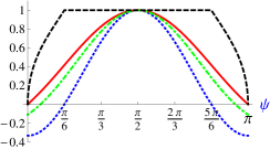
Figure 1: Color online. Parameters describing entanglement of a two–qubit pure state $\left|\Psi\right\rangle_{AB}$ as a function of the Schmidt angle $\psi$. We plot the minimal (blue/dotted), the average (green/dashed–dotted) and the maximal (red) values of the rescaled collectibility $\left[16Y_{\theta}\left(\psi\right)-1\right]/3$. Positive values identify entanglement. The black, dashed line shows the probability $P_{Y}$ that the entanglement of $\left|\Psi\right\rangle_{AB}$ is detected in a particular random measurement.

In order to characterize various possibilities to detect the entanglement we analyze four quantities. Consider first the minimal ($\theta=0$) and the maximal ($\theta=\pi/2$) value of the collectibility $Y_{\theta}\left(\psi\right)$ with respect to the detector parameters $\left(\theta,\phi\right)$,

$$Y^{min}\left(\psi\right)=\frac{\sin^{2}\left(\psi\right)}{4},\qquad Y^{max}\left(\psi\right)=\frac{\left(1+\sin\left(\psi\right)\right)^{2}}{16}.$$

Then define the mean collectibility $\overline{Y}=\langle Y_{a}\rangle_{a}$, averaged over the set of the detector parameters $a=\left(\theta,\phi\right)$ with the measure $d\Omega=\sin\left(\theta\right)d\theta\,d\phi/\left(4\pi\right)$. This case, corresponding to the average over a random choice of the detector parameters, $\overline{Y}\left(\psi\right)=\int_{\mathcal{S}^{2}}d\Omega\,Y_{\theta}\left(\psi\right)$, yields the result

$$\overline{Y}\left(\psi\right)=\frac{11-7\cos\left(2\psi\right)+3(\pi-2\psi)\tan\left(\psi\right)}{96}.$$ (16)

Furthermore, we study the probability that the entanglement is detected in a measurement with a random choice of the detector angle $\theta$, $P_{Y}\left(\psi\right)=\int_{\mathcal{P}}d\Omega$, where $\mathcal{P}=\left\{\left(\theta,\phi\right)\in\mathcal{S}^{2}:\,Y_{\theta}\left(\psi\right)>1/16\right\}$:

$$P_{Y}\left(\psi\right)=\begin{cases}\frac{\sqrt{2\sin\left(\psi\right)-\sin^{2}\left(\psi\right)}}{\left|\cos\left(\psi\right)\right|}&\textrm{ for }\psi\in\left[0,\frac{\pi}{6}\right]\cup\left[\frac{5\pi}{6},\pi\right]\\ 1&\textrm{ for }\psi\in\left[\frac{\pi}{6},\frac{5\pi}{6}\right]\end{cases}.$$ (17)

Analytical results for a pure state of the $2\times 2$ system are presented in Fig. 1. In the case of the optimal choice of the detector parameters (red curve) the entanglement is detected for any entangled state. More importantly, in the case of the worst possible choice of the measurement parameters represented by the blue/dotted curve, the entanglement is detected for $\psi\in\left[\pi/6,5\pi/6\right]$. This coincides with the fact that the probability of entanglement detection with a single random measurement is equal to unity (cf. (17) and the black, dashed curve). The average collectibility $\overline{Y}$ corresponds to an average obtained by a sequence of measurements with a random choice of the detector parameters.

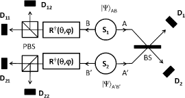
Figure 2: Determination of the Gram matrix via conditional overlapping in the case of two polarization–entangled photon pairs. Each source produces a pair of photons in a polarization state $\left|\Psi\right\rangle_{AB}$. On the left side $B$ the statistics of pairs of clicks after two PBS–elements are measured. On the right side $A$ the Hong–Ou–Mandel interference is performed. The number $|G_{12}|^{2}$ is equal to the probability of the pair of the clicks at $B$ multiplied by that of double click at $A$.

Looking at the expression (13) we see that to compute the collectibility $Y_{a}$ it is enough to determine the elements of the Gram matrix. Assume first that we analyze a two–photon polarization entangled state. The diagonal element $G_{jj}$ represents an amplitude of the state $|\varphi_{j}\rangle$ in the first subspace ${\cal H}^{A}$, under the assumption that the second photon was measured by the detector in the state $|a^{B}_{j}\rangle$. To determine the absolute value of the off diagonal element, $|G_{12}|^{2}=|\langle\varphi_{1}|\varphi_{2}\rangle|^{2}$, of the two–photon state $\left|\Psi\right\rangle_{AB}$ one projects the ${\cal H}^{B}$ part of the first copy onto the state $|a^{B}_{1}\rangle$, the same part of the second copy onto $|a^{B}_{2}\rangle$, and performs a kind of the Hong–Ou–Mandel interference experiment HOM87 with the remaining two photons of the first subsystem ${\cal H}^{A}$. A specific scheme of this kind is depicted in Fig.2.

Apart from two sources of pure entanglement (which may base on type–I PDS sources modified by dumping one of the polarization components) it involves the 50:50 beamsplitter (BS), two polarization rotators $R^{\dagger}(\theta,\phi)$ in the same setting and the polarized beamsplitters (PBS). If by $p_{ij}(+,+)$ we denote the probability of double click after the beamsplitter, and by $p_{1i}\equiv p_{1}\left((-1)^{i+1}\right)$ ($p_{2i}\equiv p_{2}\left((-1)^{i+1}\right)$) the probability of click in the $D_{1,i}$-th detector ($D_{2,i}$-th detector) i.e. one of the detectors located after upper PBS (lower PBS) then all the Gram matrix elements are:

$$|G_{ij}|^{2}=p_{1i}p_{2j}(1-2p_{ij}(+,+)).$$ (18)

Alternatively one can apply the following network designed to measure all three quantities (see Fig.3).

Figure 3: Quantum network exploiting two copies of an analyzed state $|\Psi\rangle_{AB}$, a control qubit $|c\rangle$ initially in state $|0\rangle$, controlled SWAP gate (cf. HE02 ) and two Hadamard gates. The mean value of Pauli $\sigma_{z}$ matrix of $|c\rangle$ is measured under the condition that the chosen pair $(i,j)$ of results is obtained in measurement of the same observables performed on both qubits at the bottom of the scheme.

Measuring the $\sigma_{z}$ component of the first qubit, conditioned by pair of the results $(i,j)$ (coming with probabilities $p_{1}((-1)^{i+1})$, $p_{2}((-1)^{j+1})$) of the measurements of the same ($\sigma_{z}$) observable on the last two qubits one gets an estimation of the parameter $|G_{ij}|^{2}=p_{1}((-1)^{i+1})p_{2}((-1)^{j+1})\langle\sigma_{z}\rangle_{ij}$. Without going into detailed analysis here we only mention that the purity assumption may be dropped at a price of performing two variants of the experiment each with one of two complementary (in Heisenberg sense) settings $R^{\dagger}(\theta,\phi)$, $R^{\dagger}(\theta^{\prime},\phi^{\prime})$. Then the discrimination parameter $\alpha_{K,N}=\alpha_{2,2}=1/16$ in the inequality (11) may be successfully corrected to take into account noise in Hong–Ou–Mandel interference occurring in both variants. Explicit derivation of such correction is rather complicated and will be considered in details elsewhere.

Three qubits —

Now let us investigate the case of a three qubit state ($K=3$). In this case the separability discrimination parameter is equal to $\alpha_{3,2}=1/64$. We compare a bi–separable state $|BS\rangle=|\Psi\rangle_{AB}\otimes|\phi\rangle_{C}$ and two the most important representatives, the GHZ-state and the W-state:

$$\left|GHZ\right\rangle=\frac{\left|000\right\rangle+\left|111\right\rangle}{\sqrt{2}},\quad\left|W\right\rangle=\frac{\left|001\right\rangle+\left|010\right\rangle+\left|100\right\rangle}{\sqrt{3}}.$$

Numerical results for the collectibility are compared in Table 1. We can see that the maximal and average collectibilities detect entanglement of all three states. The maximum value is attained for the GHZ-state, $Y^{\rm max}[|GHZ\rangle]=16/64$ while $Y^{\rm max}[|W\rangle]=9/64$. As this quantity for the bi–separable state reads $Y^{\rm max}[|BS\rangle]=4/64$ and $Y^{\rm max}[|\Psi_{\rm sep}\rangle]=1/64$, the collectibility offers an experimentally accessible measure capable to distinguish the genuine three–parties entanglement.

entanglement test	GHZ-state	W-state	BS-state
minimal $Y^{min}$	$0$	$0$	$0$
maximal $Y^{max}$	$0.250$	$0.141$	$0.063$
average $\overline{Y}$	$0.053$	$0.049$	$0.021$
detection probability $P_{Y}$	$0.807$	$0.807$	$0.500$

Table 1: Comparison between the GHZ-state the W-state and the bi–separable state $|BS\rangle$. We present numerical values for the minimal, maximal and average collectibilities and the probabilities $P_{Y}$ of entanglement detection in a particular, random measurement. If the values of the collectibility are larger than $1/64\approx 0.016$ then the entanglement is detected.

Acknowledgements.- It is a pleasure to thank K. Banaszek, O. Gühne, M. Kuś and M. Żukowski for fruitful discussions and helpful remarks. Financial support by the grant number N N202 174039, N N202 090239 and N N202 261938 of Polish Ministry of Science and Higher Education is gratefully acknowledged.

References

• (1) F. Mintert et al., Phys. Rep. 415, 207 (2005).
• (2) I. Bengtsson and K. Życzkowski, Geometry of quantum states: An introduction to quantum entanglement (Cambridge University Press, Cambridge, 2006).
• (3) R. Horodecki, P. Horodecki, M. Horodecki and K. Horodecki, Rev. Mod. Phys. 81, 865 (2009).
• (4) O. Gühne and G. Tóth, Phys. Rep. 474, 1 (2009).
• (5) J. Hald et al., Phys. Rev. Lett. 83, 1319 (1999); H. F. Hofmann, and S. Takeuchi, Phys. Rev. A 68, 032103 (2003); O. Gühne, Phys. Rev. Lett. 92, 117903 (2004); O. Gühne, M. Lewenstein, Phys. Rev. A 70, 022316 (2004).
• (6) M. B. Plenio, S. Virmani, Quant. Inf. Comp. 7, 1 (2007).
• (7) A. Salles et al., Phys. Rev. A 78, 022322 (2008).
• (8) P. Horodecki and A. Ekert, Phys. Rev. Lett. 89, 127902 (2002).
• (9) P. Horodecki, Phys. Rev. Lett. 90, 167901 (2003).
• (10) F. A. Bovino et al., Phys. Rev. Lett. 95, 240407 (2005).
• (11) F. Mintert et al., Phys. Rev. Lett. 95, 260502 (2005).
• (12) S.P. Walborn et al., Nature 440, 1022 (2006).
• (13) R. Augusiak and M. Lewenstein, Quantum Inf. Process. 8, 493 (2009).
• (14) H. Maassen and J. B. M. Uffink, Phys. Rev. Lett. 60, 1103 (1988).
• (15) T.-Ch. Wei et al., Phys. Rev. A 68, 042307 (2003).
• (16) D. Deutsch, Phys. Rev. Lett. 50, 631 (1983).
• (17) C. K. Hong et al., Phys. Rev. Lett. 59, 2044 (1987).