The effect of water-water hydrogen bonding on the hydrophobic hydration of macroscopic particles and its temperature dependence

Abstract.

A theoretical model for the effect of water hydrogen bonding on the thermodynamics of hydrophobic hydration is proposed as a combination of the classical density functional theory with the recently developed probabilistic approach to water hydrogen bonding in the vicinity of a hydrophobic surface. The former allows one to determine the distribution of water molecules in the vicinity of a macroscopic hydrophobic particle and calculate the thermodynamic quantities of hydrophobic hydration as well as their temperature dependence, whereas the latter allows one to implement the effect of the hydrogen bonding ability of water molecules on their interaction with the hydrophobic surface into the DFT formalism. This effect arises because the number and energy of hydrogen bonds that a water molecule forms near a hydrophobic surface differ from their bulk values. Such an alteration gives rise to a hydrogen bond contribution to the external potential field whereto a water molecule is subjected in that vicinity. This contribution is shown to play a dominant role in the interaction of a water molecule with the surface. Our approach predicts that the free energy of hydration of a planar hydrophobic surface in a model liquid water decreases with increasing temperature in the range from 293 K to 333 K. This result is indirectly supported by the counter-intuitive experimental observation that under some conditions the hydration of a molecular hydrophobe is entropically favorable as well as by the molecular dynamics simulations predicting positive hydration entropy for sufficiently large (nanoscale) hydrophobes.

1 Introduction

Particles exhibiting resistance to being either wetted by liquid water (case of meso/macroscopic ones) or dissolved therein (case of molecules) are generally referred to as hydrophobic solutes. The transfer of a hydrophobic solute into liquid water is accompanied by an increase in the free energy of the system, which results from the structural modifications of liquid water around the solute. This phenomenon is referred to as hydrophobic hydration. When two solute particles are close enough to each other, the total volume of water thus affected by both particles is smaller than when they are far apart. This gives rise to an effective, solvent-mediated (often referred to as hydrophobic) attraction between particles.

It is believed that hydrogen bonding between neighboring water molecules^1-3 constitutes a key element of hydrophobic effects ^4-7 (hydration and attraction) which, in turn, play a crucial role in many physical, chemical, and biological phenomena.^7-11 The development of predictive models capable of estimating the temperature and pressure dependence of hydrophobic phenomena is therefore quite important.

In attempts to understand hydrophobic effects at a fundamental level and to develop a generally satisfactory theory of hydrophobicity,^12,13 various mechanisms have been suggested^4-7,14-21 (mostly involving the hydrogen bonding ability of water molecules). Despite many remaining controversies, the dependence of hydrophobic phenomena on the length scales of hydrophobic particles involved appears to be out of contention.^22-25

Small hydrophobic molecules (whereof the linear size is comparable to that of a water molecule) can fit into the water hydrogen-bond network without destroying any bonds.¹⁵ One one hand, this results in a negligible enthalpy of hydration; on the other hand, the presence of the solute is thought to constrain some degrees of freedom of the neighboring water molecules which should give rise to a negative entropy of hydration proportional to the solute excluded volume. Consequently, the hydration free energy is positive and increases with temperature and solute excluded volume.

Since the hydration of small hydrophobic molecules is entropically “driven”, so is their solvent-mediatated interaction.^12,13 At small enough separations, the two hydrophobic molecules affect fewer solvent molecules than when they are far apart. Therefore, bringing two hydrophobic molecules sufficiently close enough to each other should result in a positive change of the entropy and should thereby lower the free energy of the solution (small enthalpy changes are neglected).

Although attractive owing to its simplicity, such a mechanism of small scale hydrophobicity appears to be somewhat inaccurate.^12,13 Simulations^26,27 and theory¹⁶ showed that two inert gas molecules (such as argon) would not be driven together to form a dimer; a solvent-separated pair would be a more likely state than a contact pair. This leads to a surprising suggestion that the hydration of small hydrophobic molecules is actually entropically favorable (the entropy of the system increases) which contradicts the conventional wisdom.

The hydration of large hydrophobic particles is believed to occur via a different mechanism.^12,13,27-29 When inserted into liquid water, such a particle breaks some hydrogen bonds in its immediate vicinity. This results in a large positive enthalpy of hydration and hence in a free energy change proportional to the solute surface area (as opposed to being proportional to the solute volume for small hydrophobes).

Thus, in contrast to entropically driven small-scale hydrophobicity, the hydration of large hydrophobic particles is expected to be enthalpically driven and so is their hydrophobic interaction. Fewer water hydrogen bonds have to be broken when two large hydrophobes are “in contact” than when they are far from each other, so there is a negative enthalpy change when such particles aproach each other from larger separations. The free energy change (dominated by the enthalpy change) will be hence negative and will constitute a thermodynamic driving force for their attraction.

Among theoretical means for studying hydrophobic phenomena (as well as many others including phase transitions and phase equilibria), the methods of density functional theory^30,31 (DFT) have been particularly efficient. The DFT formalism has been widely used for studying the density profiles and thermodynamic properties of fluids near rigid surfaces of various sizes, shapes, and nature.^32,33

In DFT the interaction of fluid molecules with a foreign surface is usually treated in the mean-field approximation: every fluid molecule is considered to be subjected to an external potential that arises due to its pairwise interactions with the molecules of the impenetrable substrate. This external potential gives rise to a specific contribution to the free energy functional. The minimization of the free energy functional with respect to the number density of fluid molecules (as a function of the spatial coordinate ${\bf r}$) provides their equilibrium spatial distribution. However, the effect of the impenetrable surface on the ability of fluid (water) molecules to form hydrogen bonds near the surface had been ignored so far in the conventional DFT formalism.

In the present work (that can be considered as a sequel of our recently published paper³⁴), we attempt to fill in this gap and clarify some issues concerning the hydration of large hydrophobic particles by combining the density functional theory with the recently developed probabilistic appraoch^35,36 to hydrogen bonding between water molecules in the vicinity of a foreign surface. This approach provides an analytic expression for the average number of hydrogen bonds that a water molecule can form as a function of its distance to the surface. Knowing this expression, one can implement the effect of the hydrogen bonding of water molecules on their interaction with the hydrophobic surface into DFT, which is then employed to determine the distribution of water molecules near a macroscopic hydrophobic particle and to calculate the thermodynamic quantities of hydrophobic hydration and their temperature dependence.

2 The outline of a probabilistic approach to water–water hydrogen bonding near a hydrophobic surface

Let us first briefly describe the probabilistic hydrogen bond (PHB) model^35,36 for the hydrogen bonding ability of water molecules. It considers a water molecule, whereof the location is determined by its center, to have four hydrogen-bonding (hb) arms (each capable of forming a single hydrogen bond) of rigid and symmetric (tetrahedral) configuration with the inter-arm angles $\alpha=109.47^{\circ}$. Each hb-arm can adopt a continuum of orientations. For a water molecule to form a hydrogen bond with another molecule, it is necessary that the tip of any of its hb-arms coincide with the second molecule. The length of an hb-arm thus equals the length $\eta$ of a hydrogen bond.

The hydrogen bond length $\eta$ is assumed to be independent of whether the molecules are in the bulk or near a hydrophobic surface. The characteristic length $\widetilde{\eta}$ of pairwise interactions between water and molecules constituting the substrate (flat and large enough to neglect edge effects, with its location determined by the loci of the centers of its outermost, surface molecules) plays a simple role in the hydrogen bond contribution to hydration or hydrophobic interaction.^35,36 It ($\widetilde{\eta}$) only determines the reference point for measuring the distance between water molecule and substrate, so it will be set equal to $\eta$.

Consider a “boundary” water molecule (BWM) in the vicinity of a hydrophobic substrate S (immersed in liquid water) at a distance $x$ therefrom. Such a molecule forms a smaller number of hydrogen bonds (hereafter referred to as “boundary hydrogen bonds”) than in bulk water because the hydrophobic surface restricts the configurational space available to other water molecules that are necessary for a BWM to form hydrogen bonds. The actual number of hydrogen bonds, that a particular BWM can form, depends on both its location and its orientation. A probabilistic hydrogen bond model allows one to obtain an analytic expression for the average number of bonds that a BWM can form as a function of its distance to the surface (“average” with respect to all possible orientations of the water molecule).^35,36

Note that a boundary hydrogen bond (BHB), involving at least one boundary water molecule, may be slightly altered energetically compared to the bulk one. Such alteration is still a subject of contention³⁷ as different authors suggest opposite effects, i.e., both enhancement ^18,38 and weakening^3a of the boundary hydrogen bonds. In the PHB approach, there is no restriction on the energy of a bulk (water-water) hydrogen bond, $\epsilon_{b}<0$, so that the approach is valid independent of whether $\epsilon_{b}<\epsilon_{s}$ or $\epsilon_{b}=\epsilon_{s}$, or $\epsilon_{b}>\epsilon_{s}$, where $\epsilon_{s}<0$ is the energy of a BHB.

2.1 The average number of BHB’s per water molecule

Let us choose a Cartesian coordinate system so that its $x$-axis is normal to the plate $P$ located at $x=0$. Denote the number of hydrogen bonds per bulk water molecule by $n_{b}$ and the average number of hydrogen bonds per BWM by $n_{s}$. The latter is a function of distance $x$ between the water molecule and the hydrophobic surface (assumed to be smooth on a molecular scale): $n_{s}\equiv n_{s}(x)$. If $x$ is larger than $2\eta$, the number of hydrogen bonds that the molecule can form is not affected by the presence of the surface. Therefore, $n_{s}(x)=n_{b}$ for $x\geq 2\eta$. On the other hand, the function $n_{s}(x)$ attains its minimum at the minimal distance between the water molecule and the plate, i.e., at $x=\eta$, because at this distance the configurational space available for the neighboring water molecules (to form a bond with the selected one) is restricted (compared to the bulk water) by the plate the most. The layer of thickness $\eta$ from $x=\eta$ to $x=2\eta$ is referred to as the surface hydration layer (SHL).

The function $n_{s}=n_{s}(x)$ can be shown^35,36 to have the form

$$n_{s}=k_{1}b_{1}+k_{2}b_{1}^{2}+k_{3}b_{1}^{3}+k_{4}b_{1}^{4}.$$ (1)

where $b_{1}$ is the probability that one of the hb-arms (of a bulk water molecule) can form a hydrogen bond and $k_{1}\equiv k_{1}(x),\;k_{2}\equiv k_{2}(x),\;k_{3}\equiv k_{3}(x)$, and $k_{4}\equiv k_{4}(x)$ are coefficient-functions that can be evaluated by using geometric considerations (with their dependence on the BWM orientations being averaged). The functions $k_{1}(x),k_{2}(x),k_{3}(x)$, and $k_{4}(x)$ are presented in Figure 2a of ref.36. They all become equal to $1$ at $x\geq 1$ where eq.(1) reduces to its bulk analog, $n_{b}=b_{1}+b_{1}^{2}+b_{1}^{3}+b_{1}^{4}$ (see ref.39). Since experimental data on $n_{b}$ (and even its temperature dependence) are readily available, the latter equation allows one to determine the probability $b_{1}$ as its positive solution satisfying the condition $0<b_{1}<1$. Thus, equation (1) provides an efficient pathway to $n_{s}$ as a function of $x$. Figure 2b in ref.36 presents this function for a hydrophobic flat surface immersed in water at temperature $T=293.15$ K, which corresponds to $n_{b}=3.65$ hence $b_{1}=0.963707$.

The above expression for $n_{s}$ takes into account the constraint that some orientations of the hb-arms of a BWM cannot lead to the formation of hydrogen bonds because of the proximity to the hydrophobic particle. The severity of this constraint depends on the distance of the BWM to the surface, hence the $x$-dependence of $k_{1},k_{2},k_{3},$ and $k_{4}$. It assumes that the intrinsic hydrogen-bonding ability of a BWM (i.e., the tetrahedral configuration of its hb-arms and their lengths and energies) are unaffected by its proximity to the hydrophobic surface so that the latter only restricts the configurational space available to other water molecules necessary for this BWM to form hydrogen bonds.

2.2 Hydrogen bond contribution to the interaction of a water molecule with a hydrophobic plate

Knowing the function $n_{s}(x)$, one can examine the effect of water hydrogen bonding on the hydration of hydrophobic (and even composite) particles as well as on their solvent-mediated interaction. For example, let us derive an expression for $U_{\mbox{\tiny ext}}^{\mbox{\tiny hb}}\equiv U_{\mbox{\tiny ext}}^{\mbox{\tiny hb}}(x)$, water-water hydrogen bond contribution to the total external potential field $U_{\mbox{\tiny ext}}^{\mbox{\tiny}}\equiv U_{\mbox{\tiny ext}}^{\mbox{\tiny}}(x)$ whereto a water molecule is subjected in the vicinity of a hydrophobic surface. The latter is needed for the application of DFT methods to the thermodynamics of hydrophobic phenomena.

The hydrogen bond contribution $U_{\mbox{\mbox{\tiny ext}}}^{\mbox{\mbox{\tiny hb}}}$ is due to the deviation of $n_{s}$ from $n_{b}$ (see refs.35 and 36) and the (possible) deviation of $\epsilon_{s}$ from $\epsilon_{b}$. It can be determined as

$$U_{\mbox{\tiny ext}}^{\mbox{\tiny hb}}\equiv U_{\mbox{\tiny ext}}^{\mbox{\tiny hb}}(x)=\epsilon_{s}(x)n_{s}(x)-\epsilon_{b}n_{b}\;\;\;\;\;\;\;\;\;(\eta\leq x<\infty).$$ (2)

The first term on the RHS of this equation represents the total energy of hydrogen bonds of a water molecule at a distance $x$ from the surface, whereas the second term is the energy of its hydrogen bonds in bulk (i.e., at $x\rightarrow\infty$. Note that the dependence of $U_{\mbox{\tiny ext}}^{\mbox{\tiny hb}}$ on $x$ may be due not only to the function $n_{s}(x)$, but also to the $x$-dependence of the hydrogen bond energy in the vicinity of the hydrophobic surface, $\epsilon_{s}\equiv\epsilon_{s}(x)$. In the PHB model $n_{s}(x)=n_{b}$ for $x\geq 2\eta$ hence it is reasonable to assume that $\epsilon_{s}(x)=\epsilon_{b}$ for $x\geq 2\eta$ as well. Thus, $U_{\mbox{\tiny ext}}^{\mbox{\tiny hb}}(x)$ is a very short-ranged function of $x$, such that $U_{\mbox{\tiny ext}}^{\mbox{\tiny hb}}(x)=0$ for $x\geq 2\eta$.

3 The outline of the methods of density functional theory

The effect of water-water hydrogen bonding on the density profile of (liquid) water molecules in the vicinity of a hydrophobic surface can be now examined by using DFT.^30-33 In this formalism, the grand thermodynamic potential $\Omega$ of a nonuniform single component fluid, subjected to an external potential $U_{\mbox{\tiny ext}}$, can be represented as a functional of the number density $\rho(\bf{r})$ of fluid molecules

$$\Omega[\rho({\bf r})]=\int_{V}d{\bf r}\,f_{h}(\rho({\bf r}))+\frac{1}{2}\int\int d{\bf r}d{\bf r^{\prime}}\,\rho({\bf r})\rho({\bf r^{\prime}})\phi_{\mbox{\tiny at}}(|{\bf r}-{\bf r^{\prime}}|)+\int d{\bf r}\,U_{\mbox{\tiny ext}}({\bf r})\rho({\bf r})-\mu\int d{\bf r}\,\rho({\bf r}),$$ (3)

where $V$ is the volume of the system, $\mu$ is the equilibrium chemical potential, and $\phi_{\mbox{\tiny at}}(|\bf{r}-\bf{r^{\prime}}|)$ is the attractive part of the interaction potential between two fluid molecules located at ${\bf r}$ and ${\bf r^{\prime}}$. In this expression, the contribution to the free energy due to the short range repulsive interactions (the first term on the RHS of the equation) is modeled by the hard sphere free energy in a local density approxiamtion (LDA), with $f_{h}$ at ${\bf r}$ being the Helmholtz free energy density of a hard sphere fluid of uniform density equal to $\rho({\bf r})$. The longer ranged attractive interactions are treated in a mean-field (van der Waals) approximation and represented by the second term on the RHS of eq.(3). (Note that the LDA neglects short-ranged correlations which leads to the absence of oscillations in the density profile of a fluid near a hard wall. Although more accurate, nonlocal approximations are also available,^31,40,41 we preferred the LDA to ensure the transparency of presentation and to put the emphasis on the idea of combining the DFT methods with the PHB model).

In an open thermodynamic system under conditions of constant chemical potential $\mu$, volume $V$, and temperature $T$ (grand canonical ensemble), the equilibrium density profile is obtained by minimizing the functional $\Omega[\rho(\bf{r})]$ with respect to $\rho({\bf r})$, i.e., by solving the Euler-Lagrange equation $\delta\Omega/\delta\rho=0$, which takes the form

$$\mu=\mu_{h}(\rho({\bf r}))+\int_{V}d{\bf r^{\prime}}\,\rho({\bf r^{\prime}})\phi_{\mbox{\tiny at}}(|\bf{r}-\bf{r^{\prime}}|)+U_{\mbox{\tiny ext}}({\bf r}),$$ (4)

where $\mu_{h}(\rho)\equiv df_{h}(\rho)/d\rho$ is the chemical potential of the uniform reference (hard sphere) fluid of density $\rho$. The substitution of the equilibrium density profile $\rho({\bf r})$ into eq.(3) provides the grand thermodynamic potential $\Omega$ of the fluid.

As already mentioned, the term $U_{\mbox{\tiny ext}}$ on the RHS of eq.(4) (and the corresponding term on the RHS of eq.(3)) had been conventionally meant to represent the external potential exerted by all the molecules constituting the hydrophobic substrate on a fluid molecule. Various models for the external potential were designed to take into account pairwise interactions of a fluid molecule with the molecules of the substrate^32,33 as well as the effect of the latter on the pairwise interactions between fluid molecules themselves.⁴² The contribution of these (pairwise) effects into $U_{\mbox{\tiny ext}}$ will be denoted by $U_{\mbox{\tiny ext}}^{\mbox{\tiny pw}}$ to distinguish it from the hydrogen bond contribution, $U_{\mbox{\tiny ext}}^{\mbox{\tiny hb}}$. Thus, the overall external potential whereto a water molecule is subjected near a hydrophobic surface can be represented as

$$U_{\mbox{\tiny ext}}({\bf r})=U_{\mbox{\tiny ext}}^{\mbox{\tiny pw}}({\bf r})+U_{\mbox{\tiny ext}}^{\mbox{\tiny hb}}({\bf r}).$$ (5)

In a closed thermodynamic system with constant number of molecules $N$, volume $V$, and temperature $T$ (canonical ensemble), the chemical potential $\mu$, appearing in eqs.(3) and (4), is not known in advance. Instead, it plays the role of a Lagrange multiplier corresponding to the constraint of fixed number of molecules in the system:

$$N=\int_{V}d{\bf r}\,\rho(r).$$

This equation can be used to determine the Lagrange multiplier $\mu$, i.e., chemical potential in the system, as follows (see, e.g., ref.43). Introducing the “configurational” part of the hard sphere chemical potential as $\widetilde{\mu_{h}}(\rho({\bf r}))\equiv\mu_{h}(\rho({\bf r}))-k_{B}T\ln\rho({\bf r})$, one can rewrite equation (3) in the form

$$\rho({\bf r})=\exp\Big{\{}\frac{1}{k_{B}T}\Big{[}\mu-U_{\mbox{\tiny ext}}({\bf r})-\widetilde{\mu}(\rho({\bf r^{\prime}}))-\int d{\bf r^{\prime}}\rho({\bf r^{\prime}})\phi_{\mbox{\tiny at}}(|{\bf r}-{\bf r^{\prime}}|)\Big{]}\Big{\}}.$$

Integrating this equation over the volume of the system and using the constraint on $N$, one obtains

$$\mu=k_{B}T\ln N-k_{B}T\ln\left(\int d{\bf r}\exp\Big{\{}\frac{1}{k_{B}T}\Big{[}-U_{\mbox{\tiny ext}}({\bf r})-\widetilde{\mu}(\rho({\bf r^{\prime}}))-\int d{\bf r^{\prime}}\rho({\bf r^{\prime}})\phi_{\mbox{\tiny at}}(|{\bf r}-{\bf r^{\prime}}|)\Big{]}\Big{\}}\right),$$

whereof the substitution into eq.(3) yields the Euler-Lagrange equation for the density profile in the canonical ensemble:

$$\mu_{h}(\rho({\bf r})) = k_{B}T\ln N-k_{B}T\ln\left(\int d{\bf r}\exp\Big{\{}\frac{1}{k_{B}T}\Big{[}-U_{\mbox{\tiny ext}}({\bf r})-\widetilde{\mu}(\rho({\bf r^{\prime}}))-\int d{\bf r^{\prime}}\rho({\bf r^{\prime}})\phi_{\mbox{\tiny at}}(|{\bf r}-{\bf r^{\prime}}|)\Big{]}\Big{\}}\right)$$ (6)

$$- U_{\mbox{\tiny ext}}({\bf r})-\int d{\bf r^{\prime}}\rho({\bf r^{\prime}})\phi_{\mbox{\tiny at}}(|{\bf r}-{\bf r^{\prime}}|),$$

The Helholtz free energy $F$ of the canonical ensemble can then be obtained by substituting the solution of eq.(6) into the corresponding functional of $\rho({\bf r})$:

$$F[\rho({\bf r})]=\int_{V}d{\bf r}\,f_{h}(\rho({\bf r}))+\frac{1}{2}\int\int d{\bf r}d{\bf r^{\prime}}\,\rho({\bf r})\rho({\bf r^{\prime}})\phi_{\mbox{\tiny at}}(|{\bf r}-{\bf r^{\prime}}|)+\int d{\bf r}\,U_{\mbox{\tiny ext}}({\bf r})\rho({\bf r}),$$ (7)

In the particular case of (fluid) water near a flat hydrophobic surface, one can use the planar symmetry of the system and choose the Cartesian coordinates so that the surface is located in the $y-z$ plane at $x=0$ with the molecules of the fluid occupying the “half-space” $x>0$. The eqilibrium density profile obtained from eqs.(4) or (6) is then a function of a single variable $x$, i.e., $\rho({\bf r})=\rho(x)$.

4 Free energy of hydration and its temperature dependence

In a canonical ensemble, the free energy $\Delta F_{\mbox{\tiny}}$ of hydration of a hydrophobic particle can be determined as the difference

$$\Delta F_{\mbox{\tiny}}=F-F_{0},$$ (8)

where $F$ and $F_{0}$ are the Helmholtz free energies of the system (liquid water) with and without a hydrophobic particle therein, respectively. Likewise, the free energy of hydrophobic hydration in a grand canonical ensemble can be determined as

$$\Delta\Omega_{\mbox{\tiny}}=\Omega-\Omega_{0},$$ (9)

where $\Omega$ and $\Omega_{0}$ are the values of the grand thermodynamic potential of the system (liquid water) with and without a hydrophobic particle therein, respectively.

Knowing the free energy of hydrophobic hydration, one can find $\Phi_{\mbox{\tiny S}}$ and $\Phi_{\mbox{\tiny E}}$, the entropic and energetic contributions to $\Delta F$, as

$$\Phi_{\mbox{\tiny S}}\equiv-T\Delta S_{\mbox{\tiny}}=T(\partial\Delta F_{\mbox{\tiny}}/\partial T)_{\mbox{\tiny V,N}},\;\;\;\;\;\Phi_{\mbox{\tiny E}}\equiv\Delta E_{\mbox{\tiny}}=(\partial(\Delta F_{\mbox{\tiny}}/T)/\partial(1/T))_{\mbox{\tiny V,N}},$$ (10)

respectively, such that $\Delta F_{\mbox{\tiny}}=\Phi_{\mbox{\tiny E}}+\Phi_{\mbox{\tiny S}}$ (in eq.(10) the subscripts of the partial derivatives indicate the thermodynamic variables held constant upon taking the derivatives). Clearly, for the decomposition of $\Delta F_{\mbox{\tiny}}$ into energetic and entropic components it is necessary to know its temperature dependence. (Note that a similar decomposition can be carried out for $\Delta\Omega_{\mbox{\tiny}}$.)

In the combined PHB/DFT-based model presented above, the temperature dependence of $\Delta F_{\mbox{\tiny}}$ contains a contribution from the temperature dependence of $U_{\mbox{\tiny ext}}^{\mbox{\tiny hb}}$, hydrogen bond contribution to the overall external field exerted by the hydrophobic surface on water molecules in its vicinity. As clear from eq.(2), the dependence of $U_{\mbox{\tiny ext}}^{\mbox{\tiny hb}}$ on $T$ is due to the temperature dependence of four quantities: $n_{s},\,n_{b},\,\epsilon_{s}$, and $\epsilon_{b}$. The functions $\epsilon_{b}\equiv\epsilon_{b}(T)$ and $n_{b}\equiv n_{b}(T)$ are either readily available or can be constructed on the basis of available data. On the other hand, $n_{s}$ is unambiguously related to $n_{b}$, hence its dependence on $T$ can be considered to be known as well. Finally, it is reasonable to assume that, whether in the bulk or in the surface hydration layer, the energy of a hydrogen bond depends on temperature in such a way that the ratio $\epsilon_{s}(T)/\epsilon_{b}(T)$ is independent of $T$. One can thus consider $U_{\mbox{\tiny ext}}^{\mbox{\tiny hb}}$ to be a known function of not only $x$ but also $T$, $U_{\mbox{\tiny ext}}^{\mbox{\tiny hb}}=U_{\mbox{\tiny ext}}^{\mbox{\tiny hb}}(x,T)$. This allows one to numerically determine the temperature dependence of $\Delta F_{\mbox{\tiny}}$ and to subsequently use interpolation procedure to find an accurate analytical fit thereof which then can be used in eq.(10).

5 Numerical evaluations

In order to illustrate the above model with numerical calculations, we have considered the hydration of a flat, macroscopic hydrophobic surface in a model liquid water. The pairwise interactions between two water molecules 1 and 2 were modeled with the Lennard-Jones (LJ) potential,

$$\phi_{\mbox{\tiny ww}}=4\epsilon_{\mbox{\tiny ww}}\Big{[}\Big{(}\frac{d}{r_{12}}\Big{)}^{12}-\Big{(}\frac{d}{r_{12}}\Big{)}^{6}\Big{]},$$

where $r_{12}$ is the distance between molecules 1 and 2, $\epsilon_{\mbox{\tiny ww}}$ is the energy parameter and $d$ is the diameter of a model molecule. The parameter $\epsilon_{\mbox{\tiny ww}}$ was adjusted to be $3.79\times 10^{-14}$, which differs from its values used in the computer simulations (Monte Carlo or molecular dynamics) of various water models, in which $\epsilon_{\mbox{\tiny ww}}$ ranges^3b from $5.31\times 10^{-15}$ erg (ST2 model) to $1.47\times 10^{-14}$ erg (SWM4-NDPmodel) to $2.54\times 10^{-13}$ erg (SSD model). Such a modification was needed to ensure that the phase diagram of model water more or less resembles that of real water. In the DFT formalism this can be achieved only by adjusting the single intermolecular potential describing water-water interactions , whereas in computer simulations water-water interactions are usually described by the combination of LJ and electrostatic potentials; hence the difference in the energy parameters of the respective LJ potentials. The parameter $d$ of the LJ potential also has different values in different water models^3b in the range from $3.02$ Å (SSD model) to $3.18$ Å (SWM4-NDP model). On the other hand, the length $\eta$ of the hydrogen bond (i.e., the distance between the oxygen atoms of two hydrogen-bonded water molecules) is reported^3b to be about $2.98$ Å. Since $d$’s (of various water models) and $\eta$ are so close to each other, we assumed for our model $d\simeq\eta$.

To find the equilibrium density profile of (model) water molecules in the vicinity of the hydrophobic surface, it is necessary to solve eq.(4) using, e.g., an iterative procedure.³³ Namely, the density profile $\rho_{i}(x)$at the $i^{\mbox{\tiny th}}$ iteration is found from the previous one, $\rho_{i-1}(x)$ via

$$\mu_{h}(\rho_{i}(x))=\mu-\int_{V}d{\bf r^{\prime}}\,\rho_{i-1}(x)\phi_{\mbox{\tiny at}}(|{\bf r}-{\bf r^{\prime}}|)-U_{\mbox{\tiny ext}}(x).$$ (11)

A similar iterative procedure can be used to solve equation (6),

$$\mu_{h}(\rho_{i}(x)) = k_{B}T\ln N-k_{B}T\ln\left(\int d{\bf r}\exp\Big{\{}\Big{[}-U_{\mbox{\tiny ext}}(x)-\widetilde{\mu}(\rho_{i-1}(x^{\prime}))-\int d{\bf r^{\prime}}\rho_{i-1}(x^{\prime})\phi_{\mbox{\tiny at}}(|{\bf r}-{\bf r^{\prime}}|)\Big{]}\Big{\}}\right)$$ (12)

$$- U_{\mbox{\tiny ext}}(x)-\int d{\bf r^{\prime}}\rho_{i-1}(x^{\prime})\phi_{\mbox{\tiny at}}(|\bf{r}-\bf{r^{\prime}}|).$$

For the chemical potential $\mu_{h}(\rho)\equiv\mu_{h}(\rho,T)$ of a hard sphere fluid we have adopted the well-known Carnaham-Starling approximation^32,33,44

$$\mu_{h}(\rho,T)=k_{B}T\Big{(}\ln(\Lambda^{3}\rho)+\xi\frac{8-9\xi+3\xi^{2}}{(1-\xi)^{3}}\Big{)}$$

where $\xi=(\pi d^{3}/6)\rho$ and $\Lambda=(h^{2}/2\pi mk_{B}T)^{1/2}$ is the thermal de Broglie wavelength of a model molecule of mass $m$ (with $h$ and $k_{B}$ being Planck’s and Boltzmann’s constants, respectively). Since $\mu_{h}$ is a single-valued (monotonically increasing) function of $\rho$, one can extract $\rho_{i}(x)$ from the LHS of eq.(11) or (12) and continue iterations. The attractive part $\phi_{\mbox{\tiny at}}$ of the pairwise water-water interactions was modeled by using a well-known perturbation scheme:⁴⁵

$$\phi_{\mbox{\tiny at}}(r_{12})=\left\{\begin{array}[]{ll}-\epsilon_{\mbox{\tiny ww}}&(r_{12}<2^{1/6}\eta),\\ \phi_{\mbox{\tiny ww}},&(r_{12}>2^{1/6}\eta).\end{array}\right.$$

Figure 1 presents the typical behaviour of $U_{\mbox{\tiny ext}}$ and its components. The thick dashed curve shows $U_{\mbox{\tiny ext}}$, while the lower and upper thin solid curves are for $U_{\mbox{\tiny ext}}^{\mbox{\tiny pw}}$ and $U_{\mbox{\tiny ext}}^{\mbox{\tiny hb}}$, respectively. The function $U_{\mbox{\tiny ext}}^{\mbox{\tiny pw}}(x)$ was modeled as suggested in refs.32 and 33,

$$U_{\mbox{\tiny ext}}^{\mbox{\tiny pw}}(x)=\left\{\begin{array}[]{ll}\infty&(x<\eta),\\ -\epsilon_{\mbox{\tiny sw}}\exp[-\lambda_{\mbox{\tiny sw}}\,(x-\eta)]&(x>\eta),\end{array}\right.$$ (13)

where the energy parameter $\epsilon_{\mbox{\tiny sw}}$ was taken to be equal to $k^{\mbox{\tiny}}_{\mbox{\tiny p}}\epsilon_{\mbox{\tiny ww}}$ with $k_{\mbox{\tiny p}}=2.1$ and the inverse length parameter $\lambda_{\mbox{\tiny sw}}$ was set equal to $1/\eta$ (the ratio $k^{\mbox{\tiny}}_{\mbox{\tiny p}}\equiv\epsilon_{\mbox{\tiny sw}}/\epsilon_{\mbox{\tiny ww}}$ characterizes the degree of hydrophobicity of the surface as the energy of a water molecule attraction to the surface at the distance $\eta$ between them relative to $-\epsilon_{\mbox{\tiny ww}}$). In $U_{\mbox{\tiny ext}}^{\mbox{\tiny hb}}(x)$ (see eq.(2)), the $x$-dependence of $\epsilon_{s}$ was approximated by a linear function increasing from its minimum value of $k^{\mbox{\mbox{\tiny}}}_{\mbox{\mbox{\tiny h}}}\epsilon_{b}$ at $x=\eta$ (with $k^{\mbox{\mbox{\tiny}}}_{\mbox{\mbox{\tiny h}}}=1.1$ corresponding to slightly enhanced hydrogen bonds^18,38 for molecules closest to the hydrophobic surface) to its maximum (bulk) value $\epsilon_{b}$ for $x\geq 2\eta$. This results in $U_{\mbox{\tiny ext}}^{\mbox{\tiny hb}}(x)=\epsilon_{b}n_{b}[(k^{\mbox{\mbox{\tiny}}}_{\mbox{\mbox{\tiny h}}}-(k^{\mbox{\mbox{\tiny}}}_{\mbox{\mbox{\tiny h}}}-1)(x-\eta)/\eta)n_{s}(x)/n_{b}-1]$ for $\eta\leq x<2\eta$ and $U_{\mbox{\tiny ext}}^{\mbox{\tiny hb}}(x)=0$ for $x\geq 2\eta$.

As clear from Figure 1, the hydrogen bonding contribution to the external potential has a repulsive character unlike the conventional pairwise contribution that has an attractive character (note also that the former dominates the latter in the most part of the range $\eta<x<2\eta$). The repulsive character of $U_{\mbox{\tiny ext}}^{\mbox{\tiny hb}}$ arises because that the total energy of hydrogen bonds per molecule near the hydrophobic surface is smaller (in absolute value) than in the bulk, which in turn is due to $n_{s}(x)\leq n_{b}$ and $\epsilon_{s}(x)\approx\epsilon_{b}$ for any $x$.

At a given temperature, the evaluation of the free energy of hydration is simpler in a grand canonical esemble, i.e., by solving eq.(11), substituting the resulting equilibrium density profile in eq.(3), and then calculating $\Delta\Omega_{\mbox{\tiny}}$ according to eq.(9). This procedure was applied to the hydration of an infinitely large flat hydrophobic surface in the model liduid water at temperature $T=293.15$ K and chemical potential $\mu=-11.5989$ $k_{B}T$ corresponding to the vapor-liquid equilibrium of the model fluid. The liquid state of the bulk water was ensured by imposing the appropriate boundary condition $\rho(x)\rightarrow\rho_{l}$ as $x\rightarrow\infty$ onto eq.(11), with $\rho_{l}$ being the bulk liquid density. The densities $\rho_{v}$ and $\rho_{l}$ of coexisting vapor and liquid, respectively, were found by solving a pair of equations expressing the conditions of phase equilibrium at a given $T$,

$$\left.\mu(\rho,T)\right|_{\rho=\rho_{v}}=\left.\mu(\rho,T)\right|_{\rho=\rho_{l}},\;\;\;\;\;\;\;\;\left.p(\rho,T)\right|_{\rho=\rho_{v}}=\left.p(\rho,T)\right|_{\rho=\rho_{l}},$$

where³⁴ $\mu(\rho,T)=\mu_{h}(\rho,T)-\alpha\rho$ and $p(\rho,T)=p_{h}(\rho,T)-\frac{1}{2}\alpha\rho^{2}$ and positive constant $\alpha=-\int dr\,\phi_{\mbox{\tiny at}}(r)$. The pressure of a uniform hard sphere fluid $p_{h}=p_{h}(\rho,T)$ is related to the corresponding chemical potential $\mu_{h}$ via $\partial p_{h}/\partial\rho=\rho\partial\mu_{h}/\partial\rho$. In the Carnahan-Starling approximation^34,35,41

$$p_{h}(\rho,T)=\rho k_{B}T\frac{1+\xi+\xi^{2}-\xi^{3}}{(1-\xi)^{3}}.$$

To clarify the effect of the two different contributions to $U_{\mbox{\tiny ext}}(x)$ on the water density distribution near the hydrophobe, the density profiles were obtained³⁴ by solving eq.(11) with the overall external potential a) including both pairwise and hydrogen bond contributions (i.e., $U_{\mbox{\tiny ext}}(x)=U_{\mbox{\tiny ext}}^{\mbox{\tiny pw}}(x)+U_{\mbox{\tiny ext}}^{\mbox{\tiny hb}}(x)$) and b) including only the pairwise component (i.e., with $U_{\mbox{\tiny ext}}(x)=U_{\mbox{\tiny ext}}^{\mbox{\tiny pw}}(x)$). In both cases the ratio $k^{\mbox{\tiny}}_{\mbox{\tiny p}}$ was taken to be $2.1$. It was clearly demonstrated³⁶ that the hydrogen bond contribution to the external potential plays a crucial role in the formation of a thin, “strong depletion” layer (of density much lower than liquid and of thickness of a molecular diameter, in agreement with previous suggestions^12,13) between liquid water and hydrophobic surface even for weakly hydrophobic surfaces (with high $k^{\mbox{\tiny}}_{\mbox{\tiny p}}$). It was also shown that, as expected, even for a relatively strong hydrophobic surface (with low $k^{\mbox{\tiny}}_{\mbox{\tiny p}}$) the conventional contribution to the external potential (due to pairwise interactions between a water molecule and those of the substrate) cannot cause the formation of a vapor-like layer near the surface, although it does lead to a weak decrease in the vicinal fluid denstity compared to the bulk one.

Figure 2 presents the grand canonical free energy of hydrophobic hydration $\Delta\Omega_{\mbox{\tiny}}$, expressed in units of $k_{B}T$ per $\eta^{2}$, as a function of the energetic alteration ratio $k^{\mbox{\mbox{\tiny}}}_{\mbox{\mbox{\tiny h}}}$ of hydrogen bonds (in the SHL compared to the bulk), at a constant ratio $k^{\mbox{\tiny}}_{\mbox{\tiny p}}$ (characterizing the degree of the hydrophobicity of the surface). Due to the model character of the hydrophobic surface, we considered several values of $k^{\mbox{\tiny}}_{\mbox{\tiny p}}$ (each curve in Figure 2a corresponds to a constant $k^{\mbox{\tiny}}_{\mbox{\tiny p}}=2.0,2.1,2.2$ and $2.3$ from bottom to top). As clear, the hydrophobic hydration is hardly sensitive to the hydrogen bond energy alteration ratio, $k^{\mbox{\tiny}}_{\mbox{\tiny h}}$, but quite sensitive to the degree of hydrophobicity of the surface, $k^{\mbox{\tiny}}_{\mbox{\tiny p}}$. The latter effect is also demonstrated in Figure 2b, where the dependence of $\Delta\Omega_{\mbox{\tiny}}$ on $k^{\mbox{\tiny}}_{\mbox{\tiny p}}$ is shown for the case where in eqs.(3) and (11) only the pairwise component was included in the external potential, i.e., $U_{\mbox{\tiny ext}}(x)=U_{\mbox{\tiny ext}}^{\mbox{\tiny pw}}(x)$.

The temperature effect on the strength of solvent-mediated part of hydrophobic attraction is demonstrated by Figure 3 that presents the Helmholtz free energy of hydrophobic hydration, $\Delta F_{\mbox{\tiny}}$, and its energetic and entropic components, $\Phi_{\mbox{\tiny E}}$ and $\Phi_{\mbox{\tiny S}}$, as functions of $T$. The solid curve represents $\Delta F_{\mbox{\tiny}}$ itself, while the long-dashed and short-dashed curves are for $\Phi_{\mbox{\tiny E}}$ and $\Phi_{\mbox{\tiny S}}$, respectively. All the potentials are in units of $k_{B}T$ per $\eta^{2}$. The results in Figure 3a correspond to the overall external potential in eqs.(7) and (12) that includes both the pairwise and hydrogen bond contributions (i.e., $U_{\mbox{\tiny ext}}(x)=U_{\mbox{\tiny ext}}^{\mbox{\tiny pw}}(x)+U_{\mbox{\tiny ext}}^{\mbox{\tiny hb}}(x)$), whereas Figure 3b shows the results obtained by solving eq.(12) and (7) with only the pairwise component included in the external potential (i.e., with $U_{\mbox{\tiny ext}}(x)=U_{\mbox{\tiny ext}}^{\mbox{\tiny pw}}(x)$). Both Figures 3a and 3b are for a hydrophobic surface with $k^{\mbox{\tiny}}_{\mbox{\tiny p}}=2.1$. As clear, the water hydrogen bonding plays an important role in the hydrophobic hydration by making the process thermodynamically more unfavorable (i.e.,significantly increasing the unfavorable free energy of hydration).

As shown in Figure 3, the combined PHB/DFT model predicts the free energy of hydration of a large hydrophobic particle to decrease with increasing temperature and suggests that the hydration process is enthalpically unfavorable (i.e., the enthalpic contribution to the hydration free energy is positive), but entropically favorable (i.e., the entropic contribution to the hydration free energy is negative), with the latter effect being dominant. Currently, no experimental data on the thermodynamics of hydration of large hydrophobes are available in literature. However, the enthalpic impediment to the hydration of a large hydrophobe is quite expected^12,13,27-29 (being due to the breaking of vicinal hydrogen bonds). On the other hand, while the entropic enhancement of such hydration seems somewhat counter-intuitive, there are indirect experimental and simulational indications of its physical soundness. For example, ref.44 reported experimental observation that dissolving an argon molecule in hot liquid water leads to an increase in entropy (i.e., the hydration of an argon molecule is entropically favorable), although the transfer of the same molecule into cold liquid water causes a decrease in entropy (i.e., its hydration is entropically unfavorable). These experiments are supported by a theoretical model (the two-dimensional Mercedes-Benz model with one fitting parameter)⁴⁶ as well as by the molecular dynamics simulations of SPC/E water model.⁴⁷

Furthermore, studying the lengthscale dependence of hydrophobic hydration (under various thermodynamic conditions) by means of MD simulations of SPC/E water model, it was demonstrated²³ that the hydration thermodynamics changes its character from “entropy dominated” to “enthalpy dominated” near the crossover region as the length scale of a hydrophobe increases. At $T=300$ K and pressure $-1000$ atm, the crossover region was found to be around $R=3$ nm ($R$ being the radius of a spherical hydrophobe). As reported,²³ the hydration is predominantly entropic ($\Phi_{\mbox{\tiny S}}>\Phi_{\mbox{\tiny E}}>0$), for solutes of radii smaller than $3$ nm, whereas it is predominantly enthalpic ($\Phi_{\mbox{\tiny E}}>\Phi_{\mbox{\tiny S}}>0$) for solutes of radii larger than $3$ nm. As the radius of the solute increases, the enthalpic contribution $\Phi_{\mbox{\tiny E}}$ increases whereas the entropic contribution $\Phi_{\mbox{\tiny S}}$ decreases and is expected to become negative “for sufficiently large solutes” (see ref.23). Qualitatively, this can be interpreted as the result of breaking the tetrahedrally ordered structure of water-water hydrogen bond network by the foreign hydrophobic particle; breaking the ordered structure of the hydrogen bond network is equivalent to increasing the disorder in the system which leads to an increase in its entropy.

6 Concluding remarks

In order to clarify some aspects of the effect of water-water hydrogen bonding on the thermodynamics of hydrophobic hydration, we have proposed a combination of our previously developed probabilistic approach to water-water hydrogen bonding with the classical density functional theory. The latter allows one to accurately determine the distribution of water molecules in the vicinity of a hydrophobic particle and calculate the thermodynamic quantities of hydrophobic hydration as well as their temperature dependence. The former allows one to implement the effect of the hydrogen bonding ability of water molecules on their interaction with the hydrophobic surface into the DFT formalism.

The hydrogen bond network of water molecules affects their interaction with the hydrophobic surface because the number and energy of hydrogen bonds that a water molecule forms in the the surface differ from their bulk values. Such an alteration gives rise to a short-range hydrogen bond contribution to the external potential field whereto a water molecule is subjected in that vicinity. This contribution is a dominant component of the interactions of a water molecule with the surface at distances between one and two hydrogen bond length. As we previously showed,³⁴ it plays a crucial role in the formation of a thin depletion layer (of thickness of a molecular diameter and of very low density, in agreement with previous suggestions^12,13) between liquid water and hydrophobic surface.

The combined PHB/DFT approach to hydrophobic hydration predicts that the free energy of hydration of a model hydrophobic surface in a model liquid water decreases with increasing temperature in the range from 293 K to 333 K. It also corroborates the counter-intuitive experimental, simulational, and theoretical observation that under some thermodynamic conditions the hydrophobic hydration may be entropically favorable. As a possible explanation, one can conjecture that the destruction of the tetrahedrally ordered structure of water hydrogen bond network by a hydrophobic particle results in an increased disorder in the system which leads to an increase in its entropy.

Acknowledgement - The author thanks Dr. E. Ruckenstein and Dr. G. Berim for many helpful discussions.

References

• $(1)$ Pimental, C.G.; McCellan, A.L. The Hydrogen Bond; W.H.Freeman: San Francisco, 1960.

• $(2)$ P.Schuster, G.Zindel, and C. Sandorfy (eds), The Hydrogen Bond: Recent Developments in Theory and Experiments, 3 vols (North Holland, Amsterdam, 1976).

• $(3)$ a) Chaplin, M.F. In Water of Life: The unique properties of H₂0; Lynden-Bell, R.M.; Morris, S.C.; Barrow, J.D.; Finney, J.L.; Harper, C., Eds; CRC Press, Boca Raton, 2010; p.69; b) M.F.Chaplin, Water Structure and Science, (e-Book, http://www.lsbu.ac.uk/water/index.html).

• $(4)$ Sharp, K.A. Curr. Opin. Struct. Biol. 1991, 1, 171.

• $(5)$ Soda, K. Adv. Biophys. 1993, 29, 1.

• $(6)$ Paulaitis, M.E.; Garde, S.; Ashbaugh, H.S. Curr. Opin. Colloid Interface Sci. 1996, 1, 376.

• $(7)$ Blokzijl, W.; Engberts, J.B.F.N. Angew. Chem. Int. Ed. Engl. 1993, 32, 1545-1579.

• $(8)$ Anfinsen, C.B. Science 1973, 181, 223-230.

• $(9)$ Ghelis, C.; Yan, J. Protein Folding; Academic Press: New York, 1982.

• $(10)$ Kauzmann, W. Adv.Prot.Chem. 1959, 14, 1-63.

• $(11)$ Privalov, P.L. Crit.Rev.Biochem.Mol.Biol. 1990, 25, 281-305.

• $(12)$ Ball, P. Chem.Rev. 2008, 108, 74-108.

• $(13)$ Berne, B.J.; Weeks, J.D.; Zhou, R. Annu.Rev.Phys.Chem. 2009, 60, 85-103.

• $(14)$ Frank, H.; Evans, M. J.Chem.Phys. 1945, 13, 507-532.

• $(15)$ Stillinger, F.H. J.Solut.Chem. 1973, 2, 141-158.

• $(16)$ Pratt, L.R.; D.Chandler, D. J.Chem.Phys. 1977, 67, 3683-3704.

• $(17)$ Müller, N. Accounts Chem.Res. 1990, 23, 23-28.

• $(18)$ Lee, B.; Graziano, G. J.Am.Chem.Soc. 1996, 118, 5163-5168.

• $(19)$ Widom, B.; Bhimulaparam, P.; Koga, K. Phys.Chem.Chem.Phys. 2003, 5, 3085-3093.

• $(20)$ Pratt, L.R. Annu. Rev. Phys. Chem. 2002, 53, 409-436.

• $(21)$ Lum, K.; Chandler, D.; Weeks, J.D. J.Phys.Chem.B 1999, 103, 4570-4577.

• $(22)$ Southall, N.T.; Dill, K.A. J.Phys.Chem.B 2000, 104, 1326-1331.

• $(23)$ Rajamani, S.; Truskett, T.M.; Garde, S. Proc.Natl.Acad.Sci.USA 2005, 102 9475-9480.

• $(24)$ Chandler, D. Nature 2005, 437, 640-647.

• $(25)$ Pangali, C.; Rao, M.; Berne, B.J. J.Chem.Phys. 1979, 71, 2982-2990.

• $(26)$ Watanabe, K.; Andersen, H.C. J.Phys.Chem. 1986, 90, 795-802.

• $(27)$ Lee, C.Y.; McCammon, J.A.; Rossky, P.J. J.Chem.Phys. 1984, 80, 4448-4455.

• $(28)$ Choudhury, N.; Pettitt, B.M. Mol.Simul. 2005, 31, 457-463.

• $(29)$ Choudhury, N.; Pettitt, B.M. J.Am.Chem.Soc. 2007, 129, 4847-4852.

• $(30)$ Evans, R. Adv. Phys. 1979, 28, 143-200.

• $(31)$ Evans, R. In Fundamentals of inhomogeneous fluids; Henderson, D., Ed.; Marcel Dekker: New York, 1992.

• $(32)$ Sullivan, D.E. Phys.Rev. B 1979, 20, 3991-4000.

• $(33)$ Tarazona, P.; Evans, R. Mol.Phys. 1983, 48, 799-831.

• $(34)$ Ruckenstein, E.; Djikaev, Y.S. J. Phys. Chem. Lett. 2011, 2, 1382-1386.

• $(35)$ Djikaev, Y.S.; Ruckenstein, E. J.Chem.Phys. 2010, 133, 194105.

• $(36)$ Djikaev, Y.S.; E. Ruckenstein, Curr. Opin. Colloid Interface Sci. doi:10.1016/j.cocis.2010.10.002 (2010).

• $(37)$ Meng, E.C.; Kollman, P.A. J.Phys.Chem. 1996, 110, 11460-11470.

• $(38)$ Silverstein, K.A.T.; Haymet, A.D.J.; Dill, K.A. J.Chem.Phys. 1999, 111, 8000-8009.

• $(39)$ Djikaev, Y.S.; Ruckenstein, E. J.Chem.Phys. 2009, 130, 124713.

• $(40)$ Tarazona, P. Phys. Rev. A 1985, 31, 2672-2679.

• $(41)$ Curtin, W.A.; Ashcroft, N.W. Phys. Rev. A 1985, 32, 2909-2919.

• $(42)$ Nakanishi, H.; Fisher, M.E. Phys.Rev.Lett. 1982, 49, 1565-1568.

• $(43)$ Lee, D.J.; Telo da Gama, M.M.; Gubbins, K.E. J.Chem.Phys. 1986, 85, 490-499.

• $(44)$ Carnahan, N.F.; Starling, K.E. J.Chem.Phys. 1969, 51, 635-636.

• $(45)$ Weeks, J.D.; Chandler, D.; Anderson, H.C. J.Chem.Phys. 1971, 54, 5237-5247.

• $(46)$ Xu, H.; Dill, K.A. J.Chem.Phys. 2005, 109, 23611-23617.

• $(47)$ Guillot, B.; Guissani, Y. J.Chem.Phys. 1993, 99, 8075-8094.

Captions

to Figures 1 to 3 of the manuscript “The effect of water-water hydrogen bonding on hydrophobic hydration and its temperature dependence” by Y. S. Djikaev and E. Ruckenstein.

Figure 1. The typical behaviour of the overall external potential $U_{\mbox{\tiny ext}}$ (exerted by a hydrophobic surface on water molecules in its vicinity), shown as a thick dash-dotted curve, and its components, $U_{\mbox{\tiny ext}}^{\mbox{\tiny pw}}$ (lower thin solid curve) and $U_{\mbox{\tiny ext}}^{\mbox{\tiny hb}}$ (upper thin solid curve).
Figure 2. The grand canonical free energy of hydrophobic hydration $\Delta\Omega_{\mbox{\tiny}}$, expressed in units of $k_{B}T$ per $\eta^{2}$: a) as a function of the bond energy alteration ratio $k^{\mbox{\mbox{\tiny}}}_{\mbox{\mbox{\tiny h}}}$ at a constant $k^{\mbox{\tiny}}_{\mbox{\tiny p}}$. Different curves correspond to different degrees of hydrophobicity ($k^{\mbox{\tiny}}_{\mbox{\tiny p}}=2.0,\,2.1,\,2.2$, and $2.3$ from bottom to top); b) as a function of $k^{\mbox{\tiny}}_{\mbox{\tiny p}}$ for the case where $U_{\mbox{\tiny ext}}(x)=U_{\mbox{\tiny ext}}^{\mbox{\tiny pw}}(x)$.
Figure 3. The Helmholtz free energy of hydrophobic hydration, $\Delta F_{\mbox{\tiny}}$, and its energetic and entropic components, $\Phi_{\mbox{\tiny E}}$ and $\Phi_{\mbox{\tiny S}}$, as functions of $T$ for a hydrophobic surface with $k^{\mbox{\tiny}}_{\mbox{\tiny p}}=2.1$ and a) $U_{\mbox{\tiny ext}}(x)=U_{\mbox{\tiny ext}}^{\mbox{\tiny pw}}(x)$) and b) $U_{\mbox{\tiny ext}}(x)=U_{\mbox{\tiny ext}}^{\mbox{\tiny pw}}(x)+U_{\mbox{\tiny ext}}^{\mbox{\tiny hb}}(x)$. The solid curves represent $\Delta F_{\mbox{\tiny}}$ itself, while the long-dashed and short-dashed curves are for $\Phi_{\mbox{\tiny E}}$ and $\Phi_{\mbox{\tiny S}}$, respectively.

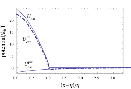
Figure 1:

$$\begin{array}[]{c@{\hspace{0.3cm}}c}\leavevmode\vspace{1.3cm}\leavevmode\hbox{a) \vspace{3cm}}\hfil\hskip 8.5359pt&\includegraphics[width=236.15796pt]{drJCPwhbdft_f5b.eps}\\[54.06006pt] \vspace{1.7cm}\leavevmode\hbox{b) \vspace{3cm}}\hfil\hskip 8.5359pt&\vspace{0.0cm}\includegraphics[width=236.15796pt]{drJCPwhbdft_f5a.eps}\\[19.91684pt] \end{array}$$

Figure 2:

$$\begin{array}[]{c@{\hspace{0.3cm}}c}\leavevmode\vspace{1.3cm}\leavevmode\hbox{a) \vspace{3cm}}\hfil\hskip 8.5359pt&\includegraphics[width=236.15796pt]{drJCPwhbdft_f4a.eps}\\[54.06006pt] \vspace{1.7cm}\leavevmode\hbox{b) \vspace{3cm}}\hfil\hskip 8.5359pt&\vspace{0.0cm}\includegraphics[width=236.15796pt]{drJCPwhbdft_f4b.eps}\\[19.91684pt] \end{array}$$

Figure 3: