Uniform Stability of a Particle Approximation of the Optimal Filter Derivative

Abstract

Sequential Monte Carlo methods, also known as particle methods, are a widely used set of computational tools for inference in non-linear non-Gaussian state-space models. In many applications it may be necessary to compute the sensitivity, or derivative, of the optimal filter with respect to the static parameters of the state-space model; for instance, in order to obtain maximum likelihood model parameters of interest, or to compute the optimal controller in an optimal control problem. In Poyiadjis et al. (2011) an original particle algorithm to compute the filter derivative was proposed and it was shown using numerical examples that the particle estimate was numerically stable in the sense that it did not deteriorate over time. In this paper we substantiate this claim with a detailed theoretical study. $\mathbb{L}_{p}$ bounds and a central limit theorem for this particle approximation of the filter derivative are presented. It is further shown that under mixing conditions these $\mathbb{L}_{p}$ bounds and the asymptotic variance characterized by the central limit theorem are uniformly bounded with respect to the time index. We demonstrate the performance predicted by theory with several numerical examples. We also use the particle approximation of the filter derivative to perform online maximum likelihood parameter estimation for a stochastic volatility model.

Some key words: Hidden Markov Models, State-Space Models, Sequential Monte Carlo, Smoothing, Filter derivative, Recursive Maximum Likelihood.

1 Introduction

State-space models are a very popular class of non-linear and non-Gaussian time series models in statistics, econometrics and information engineering; see for example Cappé et al. (2005), Doucet et al. (2001), Durbin and Koopman (2001). A state-space model is comprised of a pair of discrete-time stochastic processes, $\left\{X_{n}\right\}_{n\mathbb{\geq}0}$ and $\left\{Y_{n}\right\}_{n\geq 0}$, where the former is an $\mathcal{X}$-valued unobserved process and the latter is a $\mathcal{Y}$-valued process which is observed. The hidden process $\left\{X_{n}\right\}_{n\mathbb{\geq}0}$ is a Markov process with initial law $dx\pi_{\theta}\left(x\right)$ and time homogeneous transition law $dx^{\prime}f_{\theta}\left(\left.x^{\prime}\right|x\right)$, i.e.

$$X_{0}\sim dx_{0}\pi_{\theta}\left(x_{0}\right)\text{ and }\left.X_{n}\right|\left(X_{n-1}=x_{n-1}\right)\sim dx_{n}f_{\theta}\left(\left.x_{n}\right|x_{n-1}\right),\qquad n\geq 1.$$ (1.1)

It is assumed that the observations $\left\{Y_{n}\right\}_{n\geq 0}$ conditioned upon $\left\{X_{n}\right\}_{n\mathbb{\geq}0}$ are statistically independent and have marginal laws

$$\left.Y_{n}\right|\left(\left\{X_{k}\right\}_{k\geq 0}=\left\{x_{k}\right\}_{k\geq 0}\right)\sim dy_{n}g_{\theta}\left(\left.y_{n}\right|x_{n}\right).$$ (1.2)

Here $\pi_{\theta}\left(x\right)$, $f_{\theta}\left(\left.x\right|x^{\prime}\right)$ and $g_{\theta}\left(\left.y\right|x\right)$ are densities with respect to (w.r.t.) suitable dominating measures denoted generically as $dx$ and $dy$. For example, if $\mathcal{X}\subseteq\mathbb{R}^{p}$ and $\mathcal{Y}\subseteq\mathbb{R}^{q}$ then the dominating measures could be the Lebesgue measures. The variable $\theta$ in the densities are the particular parameters of the model. The set of possible values for $\theta$, denoted $\Theta$, is assumed to be an open subset of $\mathbb{R}^{d}$. The model (1.1)-(1.2) is also often referred to as a hidden Markov model in the literature Cappé et al. (2005).

For a sequence $\left\{z_{n}\right\}_{n\geq 0}$ and integers $i$, $j$, let $z_{i:j}$ denote the set $\left\{z_{i},z_{i+1},...,z_{j}\right\}$, which is empty if $j<i$. Equations (1.1) and (1.2) define the law of $\left(X_{0:n},Y_{0:n-1}\right)$ which is given by the measure

$$dx_{0}\pi_{\theta}\left(x_{0}\right)\prod\limits_{k=1}^{n}dx_{k}f_{\theta}\left(\left.x_{k}\right|x_{k-1}\right)\prod\limits_{k=0}^{n-1}dy_{k}g_{\theta}\left(\left.y_{k}\right|x_{k}\right),$$ (1.3)

from which the probability density of the observed process, or likelihood, is obtained

$$p_{\theta}\left(y_{0:n-1}\right)=\int dx_{0}\pi_{\theta}\left(x_{0}\right)\prod\limits_{k=1}^{n}dx_{k}f_{\theta}\left(\left.x_{k}\right|x_{k-1}\right)\prod\limits_{k=0}^{n-1}g_{\theta}\left(\left.y_{k}\right|x_{k}\right).$$ (1.4)

For a realization of observations $Y_{0:n-1}=y_{0:n-1}$, let $\mathbb{Q}_{\theta,n}$ denote the law of $X_{0:n}$ conditioned on this sequence of observed variables, i.e.

$$\mathbb{Q}_{\theta,n}(dx_{0:n})=\frac{1}{p_{\theta}\left(y_{0:n-1}\right)}\left(dx_{0}\pi_{\theta}\left(x_{0}\right)g_{\theta}\left(\left.y_{0}\right|x_{0}\right)\prod\limits_{k=1}^{n-1}dx_{k}f_{\theta}\left(\left.x_{k}\right|x_{k-1}\right)g_{\theta}\left(\left.y_{k}\right|x_{k}\right)\right)dx_{n}f_{\theta}\left(\left.x_{n}\right|x_{n-1}\right)$$

Let $\eta_{\theta,n}$ denote the time $n$ marginal of $\mathbb{Q}_{\theta,n}$. This marginal, which we call the filter, may be computed recursively using Bayes’ formula:

$$\eta_{\theta,n+1}(dx_{n+1})=\mathbb{Q}_{\theta,n+1}\left(dx_{n+1}\right)=\frac{dx_{n+1}\int\eta_{\theta,n}\left(dx_{n}\right)g_{\theta}\left(\left.y_{n}\right|x_{n}\right)f_{\theta}\left(\left.x_{n+1}\right|x_{n}\right)}{\int\eta_{\theta,n}\left(dx_{n}^{\prime}\right)g_{\theta}\left(\left.y_{n}\right|x_{n}^{\prime}\right)},\quad n\geq 0$$

and $\eta_{\theta,0}=\pi_{\theta}$ by convention. Except for simple models such the linear Gaussian state-space model or when $\mathcal{X}$ is a finite set, it is impossible to compute $p_{\theta}\left(y_{0:n}\right)$, $\mathbb{Q}_{\theta,n}$ or $\eta_{\theta,n}$ exactly. Particle methods have been applied extensively to approximate these quantities for general state-space models of the form (1.1)–(1.2); see Cappé et al. (2005), Doucet et al. (2001).

The particle approximation of $\mathbb{Q}_{\theta,n}$ is the empirical measure corresponding to a set of $N\geq 1$ random samples termed particles, that is

$$\mathbb{Q}_{\theta,n}^{\text{p},N}\left(dx_{0:n}\right)=\frac{1}{N}\sum_{i=1}^{N}\delta_{X_{0:n}^{\left(i\right)}}\left(dx_{0:n}\right)$$ (1.5)

where $\delta_{z}\left(dz\right)$ denotes the Dirac delta mass located at $z$. This approximation is referred to as the path space approximation Del Moral (2004) and it is denoted by the superscript ‘p’. The particle approximation of $\eta_{\theta,n}$ is obtained from $\mathbb{Q}_{\theta,n}^{\text{p},N}$ by marginalization

$$\eta_{\theta,n}^{N}(dx_{n})=\frac{1}{N}\sum_{i=1}^{N}\delta_{X_{n}^{\left(i\right)}}\left(dx_{n}\right).$$

These particles are propagated in time using importance sampling and resampling steps; see Doucet et al. (2001) and Cappé et al. (2005) for a review of the literature. Specifically, $\mathbb{Q}_{\theta,n+1}^{\text{p},N}$ is the empirical measure constructed from $N$ independent samples from

$$\frac{\mathbb{Q}_{\theta,n}^{\text{p},N}\left(dx_{0:n}\right)dx_{n+1}f_{\theta}\left(\left.x_{n+1}\right|x_{n}\right)g_{\theta}\left(\left.y_{n}\right|x_{n}\right)}{\int\mathbb{Q}_{\theta,n}^{\text{p},N}\left(dx_{0:n}\right)g_{\theta}\left(\left.y_{n}\right|x_{n}\right)}.$$ (1.6)

It is a well known fact that the particle approximation of $\mathbb{Q}_{\theta,n}$ becomes progressively impoverished as $n$ increases because of the successive resampling steps (Del Moral and Doucet, 2003; Olsson et al., 2008). That is, the number of distinct particles representing the marginal $\mathbb{Q}_{\theta,n}^{\text{p},N}(dx_{0:k})$ for any fixed $k<n$ diminishes as $n$ increases until it collapses to a single particle – this is known as the particle path degeneracy problem.

The focus of this paper is on the convergence properties of particle methods which have been recently proposed to approximate the derivative of the measures $\{\eta_{\theta,n}(dx_{n})\}_{n\geq 0}$ w.r.t. $\theta=[\theta_{1},\ldots\theta_{d}]^{\text{T}}\in\mathbb{R}^{d}$:

$$\zeta_{\theta,n}=\nabla\eta_{\theta,n}=\left[\frac{\partial\eta_{\theta,n}}{\partial\theta_{1}},\ldots,\frac{\partial\eta_{\theta,n}}{\partial\theta_{d}}\right]^{\text{T}}.$$

(See Section 2 for a definition.) References Cérou et al. (2001) and Doucet and Tadić (2003) present particle methods which have a computational complexity that scales linearly with the number $N$ of particles. It was shown in Poyiadjis et al. (2011) (see also Poyiadjis et al. (2009) for a more detailed numerical study) that the performance of these $\mathcal{O}(N)$ methods, which inherently rely on the particle approximations of $\{\mathbb{Q}_{\theta,n}\}_{n\geq 0}$ constructed as in (1.6) above, degraded over time and it was conjectured that this may be attributed to the particle path degeneracy problem. In contrast, the alternative method of Poyiadjis et al. (2005) was shown in numerical examples to be stable. The method of Poyiadjis et al. (2005) is a non-standard particle implementation that avoids the particle path degeneracy problem at the expense of a computational complexity per time step which is quadratic in the number of particles, i.e. $\mathcal{O}(N^{2})$; see Section 2 for more details. Supported by numerical examples, it was conjectured in Poyiadjis et al. (2011) that even under strong mixing assumptions, the variance of the estimate of the filter derivative computed with the $\mathcal{O}(N)$ methods increases at least linearly in time while that of the $\mathcal{O}(N^{2})$ is uniformly bounded w.r.t. the time index. This conjecture is confirmed in this paper. Specifically, we analyze the $\mathcal{O}(N^{2})$ implementation of Poyiadjis et al. (2005) in Section 3 and obtain results on the errors of the approximation, in particular, $\mathbb{L}_{p}$ bounds and a Central Limit Theorem (CLT) are presented. We show that these $\mathbb{L}_{p}$ bounds and asymptotic variances appearing in the CLT are uniformly bounded w.r.t. the time index when the state-space model satisfies certain mixing assumptions. In contrast, the asymptotic variance of the $\mathcal{O}(N)$ implementations, which is also captured through the CLT, is shown to increase linearly. To the best of our knowledge, these are the first results of this kind.

An important application of our results, which is discussed in detail in Section 4, is to the problem of estimating the parameters of the model (1.1)–(1.2) from observed data. The estimates of the model parameters are found by maximizing the likelihood function $p_{\theta}(y_{0:n})$ with respect to $\theta$ using a gradient ascent algorithm which relies on the particle approximation of the filter derivative. The results we present in Section 3 have bearing on the performance of the parameter estimation algorithm, which we illustrate with numerical examples in Section 4. The Appendix contains the proofs of the main results as well as that of some supporting auxiliary results. As a final remark, although the algorithms and theoretical results are presented for a state-space model, they may be reinterpreted for Feynman-Kac models as well.

1.1 Notation and definitions

We give some basic definitions from probability and operator semigroup theory. For a measurable space $(E,\mathcal{E})$ let $\mathcal{M}(E)$ denote the set of all finite signed measures and $\mathcal{P}(E)$ the set of all probability measures on $E$. The $n$-fold product space $E\times\cdots\times E$ is denoted by $E^{n}$. Let $\mathcal{B}(E)$ denote the Banach space of all bounded real-valued and measurable functions $\varphi:E\rightarrow\mathbb{R}$ equipped with the uniform norm $\|\varphi\|=\text{sup}_{x\in E}|\varphi(x)|$. For $\nu\in\mathcal{M}(E)$ and $\varphi\in\mathcal{B}(E)$, let $\nu(\varphi)=\int~{}\nu(dx)~{}\varphi(x)$ be the Lebesgue integral of $\varphi$ w.r.t. $\nu$. If $\nu$ is a density w.r.t. some dominating measure $dx$ on $E$ then, $\nu(\varphi)=\int dx$ $\nu(x)~{}\varphi(x)$. We recall that a bounded integral kernel $M(x,dx^{\prime})$ from a measurable space $(E,\mathcal{E})$ into an auxiliary measurable space $(E^{\prime},\mathcal{E}^{\prime})$ is an operator $\varphi\mapsto M(\varphi)$ from $\mathcal{B}(E^{\prime})$ into $\mathcal{B}(E)$ such that the functions

$$x\mapsto M(\varphi)(x):=\int_{E^{\prime}}M(x,dx^{\prime})\varphi(x^{\prime})$$

are $\mathcal{E}$-measurable and bounded for any $\varphi\in\mathcal{B}(E^{\prime})$. The kernel $M$ also generates a dual operator $\nu\mapsto\nu M$ from $\mathcal{M}(E)$ into $\mathcal{M}(E^{\prime})$ defined by

$$(\nu M)(\varphi):=\nu(M(\varphi)).$$

Given a pair of bounded integral operators $(M_{1},M_{2})$, we let $(M_{1}M_{2})$ the composition operator defined by $(M_{1}M_{2})(\varphi)=M_{1}(M_{2}(\varphi))$.

A Markov kernel is a positive and bounded integral operator $M$ such that $M(1)\left(x\right)=1$ for any $x\in E$. For $\varphi\in\mathcal{B}(E)$, let

$${\mbox{{\rm osc}}(}\varphi)=\sup_{x,x^{\prime}\in E}\left|\varphi(x)-\varphi(x^{\prime})\right|$$

and let

$$\mbox{Osc}_{1}(E)=\{\varphi\in\mathcal{B}(E):{\mbox{{\rm osc}}(}\varphi)\leq 1\}.$$

Let $\beta(M)\in[0,1]$ denote the Dobrushin coefficient of the Markov kernel $M$ which is defined by the formula (Del Moral, 2004, Prop. 4.2.1):

$$\beta(M):=\sup{\ \{\mbox{{\rm osc}}(M(\varphi))\;;\;\;\varphi\in\mbox{{\rm Osc}}_{1}(E^{\prime})\}.}$$

If there exists a positive constant $\rho$ such that the Markov kernel $M$ satisfies

$$M(x,dz)\geq\rho M(x^{\prime},dz)\;\text{for all}\;\,x,x^{\prime}\in E\ \,\;\text{then}\;\beta\left(M\right)\leq 1-\rho.$$

For two Markov kernels $M_{1},M_{2}$, $\beta(M_{1}M_{2})\leq\beta(M_{1})\beta(M_{2})$.

Given a positive function $G$ on $E$, let $\Psi_{G}:\nu\in\mathcal{P}(E)\mapsto\Psi_{G}(\nu)\in\mathcal{P}(E)$ be the probability distribution defined by

$$\Psi_{G}(\nu)(dx):=\frac{\nu(dx)G(x)}{\nu(G)}$$

provided $\infty>\nu(G)>0$. The definitions above also apply if $\nu$ is a density and $M$ is a transition density. In this case all instances of $\nu(dx)$ should be replaced with $dx\nu(x)$ and $M(x,dx^{\prime})$ by $dx^{\prime}M(x,x^{\prime})$ where $dx$ and $dx^{\prime}$ is generic notation for the dominating measures.

It is convenient to introduce the following transition kernels:

$$Q_{\theta,n}(x_{n-1},dx_{n}) =g_{\theta}(y_{n-1}|x_{n-1})dx_{n}f_{\theta}(x_{n}|x_{n-1})=dx_{n}q_{\theta}(x_{n}|x_{n-1}),\quad n>0,$$

$$Q_{\theta,k,n}(x_{k},dx_{n}) =\left(Q_{\theta,k+1}Q_{\theta,k+2}\cdots Q_{\theta,n}\right)(x_{k},dx_{n}),\quad 0\leq k\leq n,$$

with the convention that $Q_{\theta,n,n}=Id$, the identity operator. Note that $Q_{\theta,k,n}(1)\left(x_{k}\right)$ is the density of the law of $Y_{k:n-1}$ given $X_{k}=x_{k}$. For $0\leq p\leq n$, define the potential function $G_{\theta,p,n}$ on $\mathcal{X}$ to be

$$G_{\theta,p,n}(x_{p})=Q_{\theta,p,n}(1)(x_{p})/\eta_{\theta,p}Q_{\theta,p,n}(1).$$ (1.7)

Let the mapping $\Phi_{\theta,k,n}:\mathcal{P}(\mathcal{X})\rightarrow\mathcal{P}(\mathcal{X})$, $0\leq k\leq n$, be defined as follows

$$\Phi_{\theta,k,n}(\nu)(dx_{n})=\frac{\nu Q_{\theta,k,n}(dx_{n})}{\nu Q_{\theta,k,n}(1)}.$$

It follows that $\eta_{\theta,n}=\Phi_{\theta,k,n}(\eta_{\theta,k})$. For conciseness, we also write $\Phi_{\theta,n-1,n}$ as $\Phi_{\theta,n}$.

A key quantity that facilitates the recursive computation of the derivative of $\eta_{\theta,n}$ is the following collection of backward Markov transition kernels:

$$M_{\theta,n}(x_{n},dx_{n-1})=\frac{\eta_{\theta,n-1}(dx_{n-1})q_{\theta}(x_{n}|x_{n-1})}{\eta_{\theta,n-1}(q_{\theta}(x_{n}|\cdot))},\quad n>0.$$ (1.8)

Their particle approximations are

$$M_{\theta,n}^{N}(x_{n},dx_{n-1})=\frac{\eta_{\theta,n-1}^{N}(dx_{n-1})q_{\theta}(x_{n}|x_{n-1})}{\eta_{\theta,n-1}^{N}(q_{\theta}(x_{n}|\cdot))}.$$ (1.9)

These backward Markov kernels are convenient for computing certain conditional expectations and probability measures. In particular, for $\varphi\in\mathcal{B}(\mathcal{X}^{2})$, we have

$$\mathbb{E}_{\theta}\left[\left.\varphi\left(X_{n-1},X_{n}\right)\right|y_{0:n-1},x_{n}\right]=\int M_{\theta,n}(x_{n},dx_{n-1})\varphi\left(x_{n-1},x_{n}\right),$$

and the law of $X_{0:n-1}$ given $X_{n}=x_{n}$ and $Y_{0:n-1}=y_{0:n-1}$ is $M_{\theta,n}(x_{n},dx_{n-1})\cdots M_{\theta,1}(x_{1},dx_{0})$.

Finally, the following two definitions are needed for the CLT of the particle approximation of the derivative of $\eta_{\theta,n}$. The bounded integral operator $D_{\theta,k,n}$ from $\mathcal{X}$ into $\mathcal{X}^{n+1}$ is defined for any $F_{n}\in\mathcal{B}(\mathcal{X}^{n+1})$ by

$$D_{\theta,k,n}(F_{n})(x_{k}):=\int\left(\prod\limits_{j=k}^{1}M_{\theta,j}(x_{j},dx_{j-1})\right)\left(\prod\limits_{j=k}^{n-1}Q_{\theta,j+1}(x_{j},dx_{j+1})\right)F_{n}(x_{0:n}),\quad 0\leq k\leq n,$$ (1.10)

with the convention that $\prod\emptyset=1$. The particle approximation, $D_{\theta,k,n}^{N}$, is defined to be

$$D_{\theta,k,n}^{N}(F_{n})(x_{k}):=\int\left(\prod\limits_{j=k}^{1}M_{\theta,j}^{N}(x_{j},dx_{j-1})\right)\left(\prod\limits_{j=k}^{n-1}Q_{\theta,j+1}(x_{j},dx_{j+1})\right)F_{n}(x_{0:n}).$$ (1.11)

To be concise we write

$$\eta_{\theta,k}(dx_{k})D_{\theta,k,n}(x_{k},dx_{0:k-1},dx_{k+1:n})\quad\text{as}\quad\eta_{\theta,k}D_{\theta,k,n}(dx_{0:n}).$$

(And similarly for the particle versions.) Although convention dictates that $\eta_{\theta,k}D_{\theta,k,n}$ should be understood as the measure $(\eta_{\theta,k}D_{\theta,k,n})(dx_{0:k-1},dx_{k+1:n})$, when we mean otherwise it should be clear from the infinitesimal neighborhood.

2 Computing the filter derivative

For any $F_{n}\in\mathcal{B}(\mathcal{X}^{n+1})$, we have

$$\nabla\mathbb{Q}_{\theta,n}(F_{n})$$

$$=\frac{1}{p_{\theta}\left(y_{0:n-1}\right)}\int dx_{0:n}\nabla\left(\pi_{\theta}\left(x_{0}\right)\prod\limits_{k=1}^{n}f_{\theta}\left(\left.x_{k}\right|x_{k-1}\right)\quad\prod\limits_{k=0}^{n-1}g_{\theta}\left(\left.y_{k}\right|x_{k}\right)\right)F_{n}(x_{0:n})$$

$$\quad-\frac{1}{p_{\theta}\left(y_{0:n-1}\right)}\mathbb{E}_{\theta}\left\{\left.F_{n}(X_{0:n})\right|y_{0:n-1}\right\}\int dx_{0:n}\nabla\left(\pi_{\theta}\left(x_{0}\right)\prod\limits_{k=1}^{n}f_{\theta}\left(\left.x_{k}\right|x_{k-1}\right)\quad\prod\limits_{k=0}^{n-1}g_{\theta}\left(\left.y_{k}\right|x_{k}\right)\right)$$

$$=\mathbb{E}_{\theta}\left\{\left.F_{n}(X_{0:n})T_{\theta,n}(X_{0:n})\right|y_{0:n-1}\right\}-\mathbb{E}_{\theta}\left\{\left.F_{n}(X_{0:n})\right|y_{0:n-1}\right\}\mathbb{E}_{\theta}\left\{\left.T_{\theta,n}(X_{0:n})\right|y_{0:n-1}\right\}$$ (2.1)

where

$$T_{\theta,n}(x_{0:n}) =\sum_{k=0}^{n}t_{\theta,k}(x_{k-1},x_{k})$$ (2.2)

$$t_{\theta,k}(x_{k-1},x_{k}) =\nabla\log\left(g_{\theta}\left(\left.y_{k-1}\right|x_{k-1}\right)f_{\theta}\left(\left.x_{k}\right|x_{k-1}\right)\right),\quad k>0,$$ (2.3)

$$t_{\theta,0}(x_{-1},x_{0}) =t_{\theta,0}(x_{0})=\nabla\log\pi_{\theta}\left(x_{0}\right).$$ (2.4)

The first equality in (2.1) follows from the definition of $\mathbb{Q}_{\theta,n}$ and interchanging the order of differentiation and integration. The interchange is permissible under certain regularity conditions (Pflug, 1996); e.g. a sufficient condition would be the main assumption in Section 3 under which the uniform stability results are proved. The second equality follows from a change of measure, which then permits an importance sampling based estimator for the derivative of $\mathbb{Q}_{\theta,n}$; this is the well known score method, e.g. see Pflug (1996, Section 4.2.1). For any $\varphi_{n}\in\mathcal{B}(\mathcal{X})$, it follows by setting $F_{n}(x_{0:n})=\varphi_{n}(x_{n})$ in (2.1) that

$$\nabla\int\eta_{\theta,n}(dx_{n})\varphi_{n}(x_{n})$$

$$=\mathbb{E}_{\theta}\left\{\left.\varphi_{n}(X_{n})T_{\theta,n}(X_{0:n})\right|y_{0:n-1}\right\}-\mathbb{E}_{\theta}\left\{\left.\varphi_{n}(X_{n})\right|y_{0:n-1}\right\}\mathbb{E}_{\theta}\left\{\left.T_{\theta,n}(X_{0:n})\right|y_{0:n-1}\right\}$$

$$=\int\zeta_{\theta,n}(dx_{n})\varphi_{n}(x_{n})$$

where

$$\zeta_{\theta,n}(dx_{n})=\eta_{\theta,n}(dx_{n})\left(\mathbb{E}_{\theta}\left[\left.T_{\theta,n}\left(X_{0:n}\right)\right|y_{0:n-1},x_{n}\right]-\mathbb{E}_{\theta}\left[\left.T_{\theta,n}\left(X_{0:n}\right)\right|y_{0:n-1}\right]\right).$$ (2.5)

We call $\zeta_{\theta,n}$ the derivative of $\eta_{\theta,n}$.

Given the particle approximation (1.5) of $\mathbb{Q}_{\theta,n}$, it is straightforward to construct a particle approximation of $\zeta_{\theta,n}$:

$$\zeta_{\theta,n}^{\text{p},N}(dx_{n})=\sum_{i=1}^{N}\frac{1}{N}\left(T_{\theta,n}(X_{0:n}^{(i)})-\frac{1}{N}\sum_{j=1}^{N}T_{\theta,n}(X_{0:n}^{(j)})\right)\delta_{X_{n}^{\left(i\right)}}\left(dx_{n}\right).$$ (2.6)

This approximation is also referred to as the path space method. Such approximations were implicitly proposed in Cérou et al. (2001) and Doucet and Tadić (2003) and there are several reasons why this estimate appears attractive. Firstly, even with the resampling steps in the construction of $\mathbb{Q}_{\theta,n}^{\text{p},N}$, $\zeta_{\theta,n}^{\text{p},N}$ can be computed recursively. Secondly, there is no need to store the entire ancestry of each particle, i.e. $\left\{X_{0:n}^{\left(i\right)}\right\}_{1\leq i\leq N}$, and thus the memory requirement to construct $\zeta_{\theta,n}^{\text{p},N}$ is constant over time. Thirdly, the computational cost per time is $\mathcal{O}(N)$. However, as $\mathbb{Q}_{\theta,n}^{\text{p},N}$ suffers from the particle path degeneracy problem, we expect the approximation $\zeta_{\theta,n}^{\text{p},N}$ to worsen over time. This was indeed observed in numerical examples in Poyiadjis et al. (2011) and it was conjectured that the asymptotic variance (i.e. as $N\rightarrow\infty$) of $\zeta_{\theta,n}^{\text{p},N}$ for bounded integrands would increase linearly with $n$ even under strong mixing assumptions. This is now proven in this article.

An alternative particle method to approximate $\{\zeta_{\theta,n}\}_{n\geq 0}$ has been proposed in Poyiadjis et al. (2005, 2011). We now reinterpret this method using the representation in (2.5) and a different particle approximation of $\mathbb{Q}_{\theta,n}$ that avoids the path degeneracy problem.

The measure $\mathbb{Q}_{\theta,n}$ admits the following backward representation

$$\mathbb{Q}_{\theta,n}(dx_{0:n})=\eta_{\theta,n}(dx_{n})\prod\limits_{k=n}^{1}M_{\theta,k}(x_{k},dx_{k-1})$$

and the corresponding particle approximation of $\mathbb{Q}_{\theta,n}$ is given by

$$\mathbb{Q}_{\theta,n}^{N}(dx_{0:n})=\eta_{\theta,n}^{N}(dx_{n})\prod\limits_{k=n}^{1}M_{\theta,k}^{N}(x_{k},dx_{k-1})$$

where $M_{\theta,k}^{N}$ was defined in (1.9). This now gives rise to the following particle approximation of $\zeta_{\theta,n}$ (Poyiadjis et al., 2005, 2011):

$$\zeta_{\theta,n}^{N}(\varphi_{n})=\int\mathbb{Q}_{\theta,n}^{N}(dx_{0:n})T_{\theta,n}(x_{0:n})\left(\varphi_{n}(x_{n})-\eta_{\theta,n}^{N}(\varphi_{n})\right)$$

and indeed $\eta_{\theta,n}^{N}(\varphi_{n})=\int\mathbb{Q}_{\theta,n}^{N}(dx_{0:n})\varphi_{n}(x_{n})$. It is apparent that $\mathbb{Q}_{\theta,n}^{N}$ constructed using this backward method avoids the degeneracy in paths. It is even possible to compute $\zeta_{\theta,n}^{N}$ recursively as detailed in Algorithm 1; since a recursion for $\eta_{\theta,n}$ is already available, it is apparent from (2.5) that what remains is to specify a recursion for $\mathbb{E}_{\theta}\left[\left.T_{\theta,n}\left(X_{0:n}\right)\right|y_{0:n-1},x_{n}\right]$. Let $\overline{T}_{\theta,n}(x_{n})$ denote this term, then for $n\geq 1$,

$$\overline{T}_{\theta,n}(x_{n}) =\mathbb{E}_{\theta}\left[\left.T_{\theta,n}\left(X_{0:n}\right)\right|y_{0:n-1},x_{n}\right]$$

$$=\mathbb{E}_{\theta}\left[\left.T_{\theta,n-1}\left(X_{0:n-1}\right)\right|y_{0:n-1},x_{n}\right]+\mathbb{E}_{\theta}\left[\left.t_{\theta,n}\left(X_{n-1},X_{n}\right)\right|y_{0:n-1},x_{n}\right]$$

$$=\int M_{\theta,n}(x_{n},dx_{n-1})\left(\mathbb{E}_{\theta}\left[\left.T_{\theta,n-1}\left(X_{0:n-1}\right)\right|y_{0:n-2},x_{n-1}\right]+t_{\theta,n}\left(x_{n-1},x_{n}\right)\right)$$

$$=\int M_{\theta,n}(x_{n},dx_{n-1})\left(\overline{T}_{\theta,n-1}(x_{n-1})+t_{\theta,n}\left(x_{n-1},x_{n}\right)\right)$$

where $\overline{T}_{\theta,0}(x_{0})=t_{\theta,0}(x_{0})$. Algorithm 1 computes $\zeta_{\theta,n}^{N}$ recursively in time by computing $\left(\overline{T}_{\theta,n},\eta_{\theta,n}\right)$ and is initialized with $\overline{T}_{\theta,0}^{(i)}=t_{\theta,0}(X_{0}^{(i)})$ (see (2.2)) where $\left\{X_{0}^{\left(i\right)}\right\}_{1\leq i\leq N}$ are samples from $\pi_{\theta}(x_{0})$.

Algorithm 1: A Particle Method to Compute the Filter Derivative

$\bullet$ Assume at time $n-1$ that approximate samples $\left\{X_{n-1}^{\left(i\right)}\right\}_{1\leq i\leq N}$ from $\eta_{\theta,n-1}$ and approximations $\left\{\overline{T}_{\theta,n-1}^{(i)}\right\}_{1\leq i\leq N}$ of $\left\{\overline{T}_{\theta,n-1}\left(X_{n-1}^{\left(i\right)}\right)\right\}_{1\leq i\leq N}$ are available.

$\bullet$ At time $n$, sample $\left\{X_{n}^{\left(i\right)}\right\}_{1\leq i\leq N}$ independently from the mixture

$$\frac{\sum_{j=1}^{N}f_{\theta}\left(x_{n}|X_{n-1}^{(j)}\right)g_{\theta}\left(\left.y_{n-1}\right|X_{n-1}^{(j)}\right)}{\sum_{j=1}^{N}g_{\theta}\left(\left.y_{n-1}\right|X_{n-1}^{(j)}\right)}$$ (2.7)

and then compute $\left\{\overline{T}_{\theta,n}^{(i)}\right\}_{1\leq i\leq N}$ and $\zeta_{\theta,n}^{N}$ as follows:

$$\overline{T}_{\theta,n}^{(i)}=\frac{\sum_{j=1}^{N}\left(\overline{T}_{\theta,n-1}^{(j)}+t_{\theta,n}\left(X_{n-1}^{(j)},X_{n}^{(i)}\right)\right)f_{\theta}\left(X_{n}^{(i)}|X_{n-1}^{(j)}\right)g_{\theta}\left(\left.y_{n-1}\right|X_{n-1}^{(j)}\right)}{\sum_{j=1}^{N}f_{\theta}\left(X_{n}^{(i)}|X_{n-1}^{(j)}\right)g_{\theta}\left(\left.y_{n-1}\right|X_{n-1}^{(j)}\right)},$$ (2.8)

$$\zeta_{\theta,n}^{N}(dx_{n})=\frac{1}{N}\sum_{i=1}^{N}\left(\overline{T}_{\theta,n}^{(i)}-\frac{1}{N}\sum_{j=1}^{N}\overline{T}_{\theta,n}^{(j)}\right)\delta_{X_{n}^{\left(i\right)}}(dx_{n}).$$ (2.9)

Algorithm 1 uses the bootstrap particle filter of Gordon et al. (1993). Note that any SMC implementation of $\{\eta_{\theta,n}\}_{n\geq 0}$ may be used, e.g. the auxiliary SMC method of Pitt and Shephard (1999) or sequential importance resampling with a tailored proposal distribution (Doucet et al., 2001). It was conjectured in Poyiadjis et al. (2011) that the asymptotic variance of $\zeta_{\theta,n}^{N}(\varphi)$ for bounded integrands $\varphi$ is uniformly bounded w.r.t. $n$ under mixing assumptions. This is established in this article.

3 Stability of the particle estimates

The convergence analysis of $\zeta_{\theta,n}^{N}$ (and $\zeta_{\theta,n}^{\text{p},N}$ for performance comparison) will largely focus on the convergence analysis of the $N$-particle measures $\mathbb{Q}_{\theta,n}^{N}$ (and correspondingly $\mathbb{Q}_{\theta,n}^{\text{p},N}$) towards their limiting values $\mathbb{Q}_{\theta,n}$, as $N\rightarrow\infty$, which is in turn intimately related to the convergence of the flow of particle measures $\left\{\eta_{\theta,n}^{N}\right\}_{n\geq 0}$ towards their limiting measures $\left\{\eta_{\theta,n}\right\}_{n\geq 0}$. The $\mathbb{L}_{r}$ error bounds and the central limit theorem presented here have been derived using the techniques developed in Del Moral (2004) for the convergence analysis of the particle occupation measures $\eta_{\theta,n}^{N}$ . One of the central objects in this analysis is the local sampling errors defined as

$$V_{\theta,n}^{N}=\sqrt{N}\left(\eta_{\theta,n}^{N}-\Phi_{\theta,n}(\eta_{\theta,n-1}^{N})\right)$$ (3.1)

The fluctuation and the deviations of these centered random measures can be estimated using non-asymptotic Kintchine’s type $\mathbb{L}_{r}$-inequalities, as well as Hoeffding’s or Bernstein’s type exponential deviations (Del Moral, 2004; Del Moral and Rio, 2009). In Del Moral and Miclo (2000) it is proved that these random perturbations behave asymptotically as Gaussian random perturbations; see Lemma 7.10 in the Appendix for more details. In the proof of Theorem 7.11 (a supporting theorem) in the Appendix we provide some key decompositions expressing the deviation of the particle measures $\mathbb{Q}_{\theta,n}^{N}$ around its limiting value $\mathbb{Q}_{\theta,n}$ in terms of the local sampling errors $(V_{\theta,0}^{N},\ldots,V_{\theta,n}^{N})$. These decompositions are key to deriving the $\mathbb{L}_{r}$-mean error bounds and central limit theorems for the filter derivative.

The following regularity conditions are assumed.

(A) The dominating measures $dx$ on $\mathcal{X}$ and $dy$ on $\mathcal{Y}$ are finite, and there exist constants $0<\rho,\delta,c<\infty$ such that for all $(x,x^{\prime},y,\theta)\in\mathcal{X}^{2}\times\mathcal{Y}\times\Theta$, the derivatives of $\pi_{\theta}(x)$, $f_{\theta}\left(x^{\prime}|x\right)$ and $g_{\theta}\left(y|x\right)$ with respect to $\theta$ exists and

$$\rho^{-1}\leq f_{\theta}\left(x^{\prime}|x\right)\leq\rho,\quad\delta^{-1}\leq g_{\theta}\left(y|x\right)\leq\delta,$$ (3.2)

$$\left|\nabla\log\pi_{\theta}\left(x\right)\right|\vee\left|\nabla\log f_{\theta}\left(x^{\prime}|x\right)\right|\vee\left|\nabla\log g_{\theta}\left(y|x\right)\right|\leq c.$$ (3.3)

Admittedly, these conditions are restrictive and fail to hold for many models in practice. (Exceptions would include applications with a compact state-space.) However, they are typically made to establish the time uniform stability of particle approximations of the filter (Del Moral, 2004; Cappé et al., 2005) as they lead to simpler and more transparent proofs. Also, we observe that the behaviors predicted by the Theorems below seem to hold in practice even in cases where the state-space models do not satisfy these assumptions; see Section 4. Thus the results in this paper can be seen to provide a qualitative guide to the behavior of the particle approximation even in the more general setting.

For each parameter vector $\theta\in\Theta$, realization of observations $y=\{y_{n}\}_{n\geq 0}$ and particle number $N$, let $(\Omega,\mathcal{F},\mathbb{P}_{\theta}^{y})$ be the underlying probability space of the random process $\{(X_{n}^{(1)},\ldots,X_{n}^{(N)})\}_{n\geq 0}$ comprised of the particle system only. Let $\mathbb{E}_{\theta}^{y}$ the corresponding expectation operator computed with respect to $\mathbb{P}_{\theta}^{y}$. The first of the two main results in this section is a time uniform non-asymptotic error bound.

Theorem 3.1

Assume (A). For any $r\geq 1$, there exists a constant $C_{r}$ such that for all $\theta\in\Theta$, $y=\{y_{n}\}_{n\geq 0}$, $n\geq 0$, $N\geq 1$, and $\varphi_{n}\in\mbox{Osc}_{1}(\mathcal{X})$,

$$\sqrt{N}\mathbb{E}_{\theta}^{y}\left\{\left|\zeta_{\theta,n}^{N}(\varphi_{n})-\zeta_{\theta,n}(\varphi_{n})\right|^{r}\right\}^{\frac{1}{r}}\leq C_{r}$$

Let $\{V_{\theta,n}\}_{n\geq 0}$ be a sequence of independent centered Gaussian random fields defined as follows. For any sequence $\{\varphi_{n}\}_{n\geq 0}$ in $\mathcal{B}(\mathcal{X})$ and any $p\geq 0$, $\{V_{\theta,n}(\varphi_{n})\}_{n=0}^{p}$ is a collection of independent zero-mean Gaussian random variables with variances given by

$$\eta_{\theta,n}(\varphi_{n}^{2})-\eta_{\theta,n}(\varphi_{n})^{2}.$$ (3.4)

Theorem 3.2

Assume (A). There exists a constant $C<\infty$ such that for any $\theta\in\Theta$, $y=\{y_{n}\}_{n\geq 0}$, $n\geq 0$ and $\varphi_{n}\in\mbox{Osc}_{1}(\mathcal{X})$, $\sqrt{N}\left(\zeta_{\theta,n}^{N}-\zeta_{\theta,n}\right)(\varphi_{n})$ converges in law, as $N\rightarrow\infty$, to the centered Gaussian random variable

$$\sum_{p=0}^{n}V_{\theta,p}\left(G_{\theta,p,n}~{}\frac{D_{\theta,p,n}(F_{\theta,n}-\mathbb{Q}_{\theta,n}(F_{\theta,n}))}{D_{\theta,p,n}(1)}\right)$$ (3.5)

whose variance is uniformly bounded above by $C$ where

$$F_{\theta,n}=\left(\varphi_{n}-\mathbb{Q}_{\theta,n}(\varphi_{n})\right)\left(T_{\theta,n}-\mathbb{Q}_{\theta,n}(T_{\theta,n})\right).$$

The proofs of both these results are in the Appendix.

As a comparison, we quantify the variance of the particle estimate of the filter derivative computed using the path-based method (see (2.6).) Consider the following simplified example that serves to illustrate the point. Let $g_{\theta}\left(\left.y\right|x\right)=g\left(\left.y\right|x\right)$ (that is $\theta$-independent), $f_{\theta}\left(\left.x_{n}\right|x_{n-1}\right)=\pi_{\theta}(x_{n})$, where $\pi_{\theta}$ is the initial distribution. (Note that $f_{\theta}$ in this case satisfies a rephrased version of (3.2) under which the conclusion of Theorem 3.2 also holds.) Also, consider the sequence of repeated observations $y_{0}=y_{1}=\cdots$ where $y_{0}$ is arbitrary. Applying Lemma 7.12 (in the Appendix) that characterizes the limiting distribution of $\sqrt{N}(\mathbb{Q}_{\theta,n}^{\text{p},N}-\mathbb{Q}_{\theta,n})$ to this special case results in $\sqrt{N}(\zeta_{\theta,n}^{\text{p},N}-\zeta_{\theta,n})(\varphi)$ (see (2.6)) having an asymptotic distribution which is Gaussian with mean zero and variance

$$n\ \times\pi_{\theta}(\overline{\varphi}^{2})\pi_{\theta}^{\prime}\left[(\nabla\log\pi_{\theta})^{2}\right]+\pi_{\theta}\left[\overline{\varphi}^{2}(\nabla\log\pi_{\theta})^{2}\right]-\nabla\pi_{\theta}(\varphi)^{2}$$

where $\overline{\varphi}=\varphi-\pi_{\theta}(\varphi)$, $\pi_{\theta}^{\prime}(x)=\pi_{\theta}(x)g\left(\left.y_{0}\right|x\right)/\pi_{\theta}\left(g\left(\left.y_{0}\right|\cdot\right)\right)$. This variance increases linearly with time in contrast to the time bounded variance of Theorem 3.2.

4 Application to recursive parameter estimation

Being able to compute $\{\zeta_{\theta,n}\}_{n\geq 0}$ is particularly useful when performing online static parameter estimation for state-space models using Recursive Maximum Likelihood (RML) techniques (Le Gland and Mevel, 1997; Poyiadjis et al., 2005, 2011); see also Kantas et al. (2009) for a general review of available particle methods based solutions, including Bayesian ones, for this problem. The computed filter derivative may also be useful in other areas; e.g. see Coquelin et al. (2008) for an application in control.

4.1 Recursive Maximum Likelihood

Let $\theta^{\ast}$ be the true static parameter generating the observed data $\{y_{n}\}_{n\geq 0}$. Given a finite record of observations $y_{0:T}$, the log-likelihood may be maximized with the following steepest ascent algorithm:

$$\theta_{k}=\theta_{k-1}+\gamma_{k}\left.\nabla\log p_{\theta}(y_{0:T})\right|_{\theta=\theta_{k-1}},\quad k\geq 1,$$ (4.1)

where $\theta_{0}$ is some arbitrary initial guess of $\theta^{\ast}$, $\left.\nabla\log p_{\theta}(y_{0:T})\right|_{\theta=\theta_{k-1}}$ denotes the gradient of the log-likelihood evaluated at the current parameter estimate and $\{\gamma_{k}\}_{k\geq 1}$ is a decreasing positive real-valued step-size sequence, which should satisfy the following constraints:

$$\sum_{k=1}^{\infty}\gamma_{k}=\infty,\qquad\sum_{k=1}^{\infty}\gamma_{k}^{2}<\infty.$$

Although $\nabla\log p_{\theta}(y_{0:T})$ can be computed using (4.3), the computation cost can be prohibitive for a long data record since each iteration of (4.1) would require a complete browse through the $T+1$ data points. A more attractive alternative would be a recursive procedure in which the data is run through once only sequentially. For example, consider the following update scheme:

$$\theta_{n}=\theta_{n-1}+\gamma_{n}\left.\nabla\log p_{\theta}(y_{n}|y_{0:n-1})\right|_{\theta=\theta_{n-1}}$$ (4.2)

where $\left.\nabla\log p_{\theta}(y_{n}|y_{0:n-1})\right|_{\theta=\theta_{n-1}}$ denotes the gradient of $\log p_{\theta}(y_{n}|y_{0:n-1})$ evaluated at the current parameter estimate; that is upon receiving $y_{n}$, $\theta_{n-1}$ is updated in the direction of ascent of the conditional density of this new observation. Since we have

$$\left.\nabla\log p_{\theta}(y_{n}|y_{0:n-1})\right|_{\theta=\theta_{n-1}}=\frac{\int dx_{n}\eta_{\theta_{n-1},n}(x_{n})\left.\nabla g_{\theta}\left(\left.y_{n}\right|x_{n}\right)\right|_{\theta_{n-1}}+\int dx_{n}\left(\left.y_{n}\right|x_{n}\right)\zeta_{\theta_{n-1},n}(x_{n})g_{\theta_{n-1}}}{\int dx_{n}\eta_{\theta_{n-1},n}(x_{n})g_{\theta_{n-1}}\left(\left.y_{n}\right|x_{n}\right)},$$ (4.3)

this clearly requires the filter derivative $\zeta_{\theta,n}$. The algorithm in the present form is not suitable for online implementation as it requires re-computing the filter and its derivative at the value $\theta=\theta_{n-1}$ from time zero. The RML procedure uses an approximation of (4.3) which is obtained by updating the filter and its derivative using the parameter value $\theta_{n-1}$ at time $n$; we refer the reader to Le Gland and Mevel (1997) for details. The asymptotic properties of the RML algorithm, i.e. the behavior of $\theta_{n}$ in the limit as $n$ goes to infinity, has been studied in the case of an i.i.d. hidden process by Titterington (1984) and Le Gland and Mevel (1997) for a finite state-space hidden Markov model. It is shown in Le Gland and Mevel (1997) that under regularity conditions this algorithm converges towards a local maximum of the average log-likelihood and that this average log-likelihood is maximized at $\theta^{\ast}$. A particle version of the RML algorithm of Le Gland and Mevel (1997) that uses Algorithm 1’s estimate of $\eta_{\theta,n}$ is presented as Algorithm 2.

Algorithm 2: Particle Recursive Maximum Likelihood

$\bullet$ At time $n-1$ we are given $y_{0:n-1}$, the previous estimate $\theta_{n-1}$ of $\theta^{\ast}$ and $\{(X_{n-1}^{\left(i\right)},\overline{T}_{n-1}^{(i)})\}_{i=1}^{N}$.

$\bullet$ At time $n$, upon receiving $y_{n}$, sample $\left\{X_{n}^{\left(i\right)}\right\}_{1\leq i\leq N}$ independently from (2.7) using parameter $\theta=\theta_{n-1}$ to obtain

$$\eta_{n}^{N}(dx_{n})=\frac{1}{N}\sum_{i=1}^{N}\delta_{X_{n}^{\left(i\right)}}(dx_{n})$$

and then compute

$$\overline{T}_{n}^{(i)}=\frac{\sum_{j=1}^{N}\left(\overline{T}_{n-1}^{(j)}+t_{\theta_{n-1},n}\left(X_{n-1}^{(j)},X_{n}^{(i)}\right)\right)f_{\theta_{n-1}}\left(X_{n}^{(i)}|X_{n-1}^{(j)}\right)g_{\theta_{n-1}}\left(\left.y_{n-1}\right|X_{n-1}^{(j)}\right)}{\sum_{j=1}^{N}f_{\theta_{n-1}}\left(X_{n}^{(i)}|X_{n-1}^{(j)}\right)g_{\theta_{n-1}}\left(\left.y_{n-1}\right|X_{n-1}^{(j)}\right)},$$ (4.4)

$$\zeta_{n}^{N}(dx_{n})=\frac{1}{N}\sum_{i=1}^{N}\left(\overline{T}_{n}^{(i)}-\frac{1}{N}\sum_{j=1}^{N}\overline{T}_{n}^{(j)}\right)\delta_{X_{n}^{\left(i\right)}}(dx_{n}),$$ (4.5)

and

$$\widehat{\nabla}\log p\left(\left.y_{n}\right|y_{0:n-1}\right)=\frac{\int\eta_{n}^{N}(dx_{n})\left.\nabla g_{\theta}\left(\left.y_{n}\right|x_{n}\right)\right|_{\theta_{n-1}}+\int\zeta_{n}^{N}(dx_{n})g_{\theta_{n-1}}\left(\left.y_{n}\right|x_{n}\right)}{\int\eta_{n}^{N}(dx_{n})g_{\theta_{n-1}}\left(\left.y_{n}\right|x_{n}\right)}.$$

Finally update the parameter:

$$\theta_{n}=\theta_{n-1}+\gamma_{n}\widehat{\nabla}\log p\left(\left.y_{n}\right|y_{0:n-1}\right).$$ (4.6)

Under Assumption A, the particle approximation of the filter is stable (Del Moral, 2004); see also Lemma 7.4 in the Appendix. This combined with the proven stability of the particle approximation of the filter derivative implies that the particle estimate of the derivative of $\log p\left(\left.y_{n}\right|y_{0:n-1}\right)$ is also stable.

4.2 Simulations

The RML algorithm is applied to the following stochastic volatility model (Pitt and Shephard, 1999):

$$X_{0} \sim\mathcal{N}\left(0,\frac{\sigma^{2}}{1-\phi^{2}}\right),\text{ }X_{n+1}=\phi X_{n}+\sigma V_{n+1},$$

$$Y_{n} =\beta\exp\left(X_{n}/2\right)W_{n},$$

where $\mathcal{N}\left(m,s\right)$ denotes a Gaussian random variable with mean $m$ and variance $s$, $V_{n}\overset{\text{i.i.d.}}{\sim}\mathcal{N}\left(0,1\right)$ and $W_{n}\overset{\text{i.i.d.}}{\sim}\mathcal{N}\left(0,1\right)$ are two mutually independent sequences, both independent of the initial state $X_{0}$. The model parameters, $\theta=\left(\phi,\sigma,\beta\right)$, are to be estimated.

Our first example demonstrates the theoretical results in Section 3. The estimate of $\partial/\partial\sigma$ $\log p\left(\left.y_{n:n+L-1}\right|y_{0:n-1}\right)$ at $\theta^{\ast}=(0.8,\sqrt{0.1},1)$  was computed using Algorithm 1 with 500 particles and using the path-space method (see (2.6)) with $2.5\times 10^{5}$ particles for the stochastic volatility model. The block size $L$ was 500. Shown in Figure 1 is the variance of these particle estimates for various values of $n$ derived from many independent random replications of the simulation. The linear increase of the variance of the path-space method as predicted by theory is evident although Assumption A is not satisfied.

For the path-space method, because the variance of the estimate of the filter derivative grows linearly in time, the eventual high variance in the gradient estimate can result in the divergence of the parameter estimates. To illustrate this point, (4.6) was implemented with the path-space estimate of the filter derivative (2.6) computed with 10000 particles and constant step-size sequence, $\gamma_{n}=10^{-4}$ for all $n$. $\theta_{0}$ was initialized at the true parameter value. A sequence of two million observations was simulated with $\theta^{\ast}=(0.8,\sqrt{0.1},1)$. The results are shown in Figure 3.

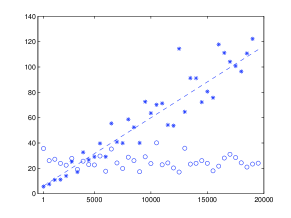
Figure 1: Variance of the particle estimates of $\partial/\partial\sigma\log p\left(\left.y_{n:n+500-1}\right|y_{0:n-1}\right)$ for various values of $n$ for the stochastic volatility model. Circles are variance of Algorithm 1’s estimate with 500 particles. Stars indicate the variance of the estimate of the path-space method with $2.5\times 10^{5}$ particles. Dotted line is best fitting straight line to path-space method’s variance to indicate trend.

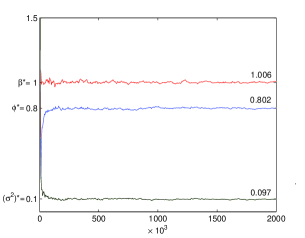
Figure 2: Sequence of recursive parameter estimates, $\theta_{n}=\left(\sigma_{n},\phi_{n},\beta_{n}\right)$, computed using (4.6) with $N=500$. From top to bottom: $\beta_{n}$, $\phi_{n}$ and $\sigma_{n}$ and marked on the right are the “converged values” which were taken to be the empirical average of the last 1000 values.

For the same value of $\theta^{\ast}$ and sequence of observations used in the previous example, Algorithm 2 was executed with 500 particles and $\gamma_{n}=0.01$, $n\leq 10^{5}$, $\gamma_{n}=(n-5\times 10^{4})^{-0.6}$, $n>10^{5}$. As it can be seen from the results in Figure 2 the estimate converges to a value in the neighborhood of the true parameter.

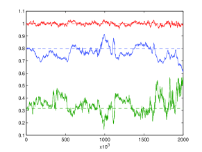
Figure 3: RML for stochastic volatility with path-space gradient estimate with 10,000 particles, constant step-size and initialized at the true parameter values which are indicated by the dashed lines. From top to bottom, $\phi$, $\beta$ and $\sigma$.

5 Conclusion

We have presented theoretical results establishing the uniform stability of the particle approximation of the optimal filter derivative proposed in Poyiadjis et al. (2005, 2009). While these results have been presented in the context of state-space models, they can also be applied to Feynman-Kac models (Del Moral, 2004) which could potentially enlarge the range of applications. For example, if $dx^{\prime}f_{\theta}\left(\left.x^{\prime}\right|x\right)$ is reversible w.r.t. to some probability measure $\mu_{\theta}$ and if we replace $g_{\theta}\left(\left.y_{n}\right|x_{n}\right)$ with a time-homogeneous potential function $g_{\theta}\left(x_{n}\right)$ then $\eta_{\theta,n}$ converges, as $n\rightarrow\infty$, to the probability measure $\mu_{\theta,h}$ defined as

$$\mu_{\theta,h}(dx):=\frac{1}{\mu_{\theta}(h_{\theta}\text{ }\int dx^{\prime}f_{\theta}\left(\left.x^{\prime}\right|\cdot\right)h_{\theta}(x^{\prime}))}\mu_{\theta}(dx)~{}h_{\theta}(x)~{}\int dx^{\prime}f_{\theta}\left(\left.x^{\prime}\right|x\right)h_{\theta}(x^{\prime})$$

where $h_{\theta}$ is a positive eigenmeasure associated with the top eigenvalue of the integral operator $Q_{\theta}(x,dx^{\prime})=g_{\theta}(x)dx^{\prime}f_{\theta}\left(\left.x^{\prime}\right|x\right)$ (see section 12.4 of Del Moral (2004)). The measure $\mu_{\theta,h}$ is the invariant measure of the $h$-process defined as the Markov chain with transition kernel $M_{\theta}\left(x,dx^{\prime}\right)\propto dx^{\prime}f_{\theta}\left(\left.x^{\prime}\right|x\right)h_{\theta}(x^{\prime})$. The particle algorithm described here can be directly used to approximate the derivative of this invariant measure w.r.t to $\theta$. It would also be of interest to weaken Assumption A and there are several ways this might be approached. For example for non-ergodic signals using ideas in Oudjane and Rubenthaler (2005); Heine and Crisan (2008) or via Foster-Lyapunov conditions as in Beskos et al. (2011); Whiteley (2011).

6 Acknowledgement

We are grateful to Sinan Yildirim for carefully reading this report.

7 Appendix

The statement of the results in this section hold for any $\theta$ and any sequence of observations $y=\{y_{n}\}_{n\geq 0}$. All mathematical expectations are taken with respect to the law of the particle system only for the specific $\theta$ and $y$ under consideration. While $\theta$ is retained in the statement of the results, it is omitted in the proofs. The superscript $y$ of the expectation operator is also omitted in the proofs.

This section commences with some essential definitions in addition to those in Section 1.1. Let

$$P_{\theta,k,n}(x_{k},dx_{n})=\frac{Q_{\theta,k,n}(x_{k},dx_{n})}{Q_{\theta,k,n}(1)(x_{k})},$$

and

$$\mathcal{M}_{\theta,p}(x_{p},dx_{0:p-1})=\prod\limits_{k=p}^{1}M_{\theta,k}(x_{k},dx_{k-1}),\quad p>0,$$

and its corresponding particle approximation is

$$\mathcal{M}_{\theta,p}^{N}(x_{p},dx_{0:p-1})=\prod\limits_{k=p}^{1}M_{\theta,k}^{N}(x_{k},dx_{k-1})$$

To make the subsequent expressions more terse, let

$$\widetilde{\eta}_{\theta,n}^{N}=\Phi_{\theta,n}(\eta_{\theta,n-1}^{N}),\quad n\geq 0,$$ (7.1)

where $\widetilde{\eta}_{\theta,0}^{N}=\Phi_{\theta,0}(\eta_{-1}^{N})=\eta_{\theta,0}=\pi_{\theta}$ by convention. (Recall $\Phi_{\theta,n}=\Phi_{\theta,n-1,n}$.) Let

$$\mathcal{F}_{n}^{N}=\sigma\left(\left\{X_{k}^{(i)};0\leq k\leq n,1\leq i\leq N\right\}\right),\quad n\geq 0,$$

be the natural filtration associated with the $N$-particle approximation model and let $\mathcal{F}_{-1}^{N}$ be the trivial sigma field.

The following estimates are a straightforward consequence of Assumption (A). For all $\theta$ and time indices $0\leq k<q\leq n$,

$$b_{\theta,k,n}=\sup_{x_{k},x_{k}^{\prime}}{\frac{Q_{\theta,k,n}(1)(x_{k})}{Q_{\theta,k,n}(1)(x_{k}^{\prime})}}\leq\rho^{2}\delta^{2},\quad\beta\left(\frac{Q_{\theta,k,q}(x_{k},dx_{q})Q_{\theta,q,n}(1)(x_{q})}{Q_{\theta,k,q}(Q_{\theta,q,n}(1))(x_{k})}\right)\leq\left(1-\rho^{-4}\right)^{(q-k)}=\overline{\rho}^{q-k},$$ (7.2)

and for $\theta$, $0<k\leq q$,

$$M_{\theta,k}^{N}(x,dz)\leq\rho^{4}~{}M_{\theta,k}^{N}(x^{\prime},dz)\Longrightarrow\beta\left(M_{\theta,q}^{N}\cdots M_{\theta,k}^{N}\right)\leq\left(1-\rho^{-4}\right)^{q-k+1}.$$ (7.3)

Note that setting $q=n$ in (7.2) yields an estimate for $\beta(P_{\theta,k,n})$

Several auxiliary results are now presented, all of which hinge on the following Kintchine type moment bound proved in Del Moral (2004, Lem. 7.3.3).

Lemma 7.1

Del Moral (2004, Lemma 7.3.3)Let $\mu$ be a probability measure on the measurable space $(E,\mathcal{E})$. Let $G$ and $h$ be $\mathcal{E}$-measurable functions satisfying $G(x)\geq cG(x^{\prime})>0$ for all $x,x^{\prime}\in E$ where $c$ is some finite positive constant. Let $\{X^{(i)}\}_{1\leq i\leq N}$ be a collection of independent random samples from $\mu$. If $h$ has finite oscillation then for any integer $r\geq 1$ there exists a finite constant $a_{r}$, independent of $N$, $G$ and $h$, such that

$$\sqrt{N}\mathbb{E}\left\{\left|\frac{\sum_{i=1}^{N}G(X^{(i)})h(X^{(i)})}{\sum_{i=1}^{N}G(X^{(i)})}-\frac{\mu(Gh)}{\mu(G)}\right|^{r}\right\}^{\frac{1}{r}}\leq c^{-1}\mbox{\rm osc}(h)a_{r}.$$

Proof:
The result for $G=1$ and $c=1$ is proved in Del Moral (2004). The case stated here can be established using the representation

$$\frac{\mu^{N}(Gh)}{\mu^{N}(G)}-\frac{\mu(Gh)}{\mu(G)}=\frac{\mu(G)}{\mu^{N}(G)}\left(\mu^{N}-\mu\right)\left[\frac{G}{\mu(G)}\left(h-\frac{\mu(Gh)}{\mu(G)}\right)\right]$$

where $\mu^{N}(dx)=N^{-1}\sum_{i=1}^{N}\delta_{X^{(i)}}(dx)$.

Remark 7.2

For $k\geq 0$, let $h_{k-1}^{N}$ be a $\mathcal{F}_{k-1}^{N}\$measurable function satisfying $h_{k-1}^{N}\in\mbox{Osc}_{1}(\mathcal{X})$ almost surely. Then Lemma 7.1 can be invoked to establish

$$\sqrt{N}\mathbb{E}_{\theta}^{y}\left\{\left|\frac{\eta_{\theta,k}^{N}(Gh_{k-1}^{N})}{\eta_{\theta,k}^{N}(G)}-\frac{\Phi_{\theta,k}(\eta_{\theta,k-1}^{N})(Gh_{k-1}^{N})}{\Phi_{\theta,k}(\eta_{\theta,k-1}^{N})(G)}\right|^{r}\right\}^{\frac{1}{r}}\leq c^{-1}a_{r}$$

where $G$ is defined as in Lemma 7.1.

Lemma 7.3 to Lemma 7.6 are a consequence of Lemma 7.1 and the estimates in (7.2).

Lemma 7.3

For any $r\geq 1$ there exist a finite constant $a_{r}$ such that the following inequality holds for all $\theta$, $y$, $0\leq k\leq n$ and $\mathcal{F}_{k-1}^{N}\$measurable function $\varphi_{n}^{N}$ satisfying$\ \varphi_{n}^{N}\in\mbox{Osc}_{1}(\mathcal{X})$
almost surely,

$$\sqrt{N}\mathbb{E}_{\theta}^{y}\left(\left|\Phi_{\theta,k,n}(\eta_{\theta,k}^{N})(\varphi_{n}^{N})-\Phi_{\theta,k-1,n}(\eta_{\theta,k-1}^{N})(\varphi_{n}^{N})\right|^{r}~{}~{}\right)^{\frac{1}{r}}\leq a_{r}~{}b_{\theta,k,n}~{}\beta\left(P_{\theta,k,n}\right),$$

where, by convention $\Phi_{\theta,-1,n}(\eta_{\theta,-1}^{N})=\eta_{\theta,n}$, and the constants $~{}b_{\theta,k,n}~{}$and $\beta\left(P_{\theta,k,n}\right)$ were defined in (7.2).

Proof:

$$\Phi_{k,n}(\eta_{k}^{N})(\varphi_{n}^{N})-\Phi_{k-1,n}(\eta_{k-1}^{N})(\varphi_{n}^{N})$$

$$=\int\left(\frac{\eta_{k}^{N}(dx_{k})Q_{k,n}(1)(x_{k})}{\eta_{k}^{N}Q_{k,n}(1)}-\frac{\Phi_{k}(\eta_{k-1}^{N})(dx_{k})Q_{k,n}(1)(x_{k})}{\Phi_{k}(\eta_{k-1}^{N})Q_{k,n}(1)}\right)P_{k,n}(\varphi_{n}^{N})(x_{k})$$

where $\Phi_{0}(\eta_{-1}^{N})=\eta_{0}$ by convention. Applying Lemma 7.1 with the estimates in (7.2) we have

$$\sqrt{N}\mathbb{E}\left(\left|\Phi_{k,n}(\eta_{k}^{N})(\varphi_{n}^{N})-\Phi_{k-1,n}(\eta_{k-1}^{N})(\varphi_{n}^{N})\right|^{r}~{}\left|~{}\mathcal{F}_{k-1}^{N}\right.\right)^{\frac{1}{r}}\leq a_{r}~{}b_{k,n}~{}\beta\left(P_{k,n}\right)$$

almost surely.

Lemma 7.3 may be used to derive the following error estimate (Del Moral, 2004, Theorem 7.4.4).

Lemma 7.4

For any $r\geq 1$, there exists a constant $c_{r}$ such that the following inequality holds for all $\theta$, $y$, $n\geq 0$ and $\varphi\in\mbox{Osc}_{1}(\mathcal{X})$,

$$\sqrt{N}\mathbb{E}_{\theta}^{y}\left(\left|[\eta_{\theta,n}^{N}-\eta_{\theta,n}](\varphi)\right|^{r}\right)^{\frac{1}{r}}\leq c_{r}~{}\sum_{k=0}^{n}~{}b_{\theta,k,n}~{}\beta\left(P_{\theta,k,n}\right).$$ (7.4)

Assume (A). For any $r\geq 1$, there exists a constant $c_{r}^{\prime}$ such that for all $\theta$, $y$, $n\geq 0$, $\varphi\in\mbox{Osc}_{1}(\mathcal{X})$, $G\in\mathcal{B}(\mathcal{X})$ such that $G$ is positive and satisfies $G(x)\geq c_{G}G(x^{\prime})$ for all $x,x^{\prime}\in\mathcal{X}$ for some positive constant $c_{G}$,

$$\sqrt{N}\mathbb{E}_{\theta}^{y}\left(\left|\left[\frac{\eta_{\theta,n}^{N}(dx_{n})G(x_{n})}{\eta_{\theta,n}^{N}(G)}-\frac{\eta_{\theta,n}(dx_{n})G(x_{n})}{\eta_{\theta,n}(G)}\right]\left(\varphi\right)\right|^{r}\right)^{\frac{1}{r}}\leq c_{r}^{\prime}(1+c_{G}^{-1}).$$ (7.5)

Proof:
The first part follows from applying Lemma 7.3 to the telescopic sum (Del Moral, 2004, Theorem 7.4.4):

$$\left(\eta_{n}^{N}-\eta_{n}\right)(\varphi)=\sum\limits_{k=0}^{n}\Phi_{k,n}(\eta_{k}^{N})(\varphi)-\Phi_{k-1,n}(\eta_{k-1}^{N})(\varphi)$$

with the convention that $\Phi_{-1,n}(\eta_{-1}^{N})=\eta_{n}$. For the second part, use the same telescopic sum but with the $k$-th term being

$$\frac{\Phi_{k,n}(\eta_{k}^{N})(\varphi G)}{\Phi_{k,n}(\eta_{k}^{N})(G)}-\frac{\Phi_{k-1,n}(\eta_{k-1}^{N})(\varphi G)}{\Phi_{k-1,n}(\eta_{k-1}^{N})(G)}$$

$$=\int\left(\frac{\eta_{k}^{N}(dx_{k})Q_{k,n}(G)(x_{k})}{\eta_{k}^{N}Q_{k,n}(G)}-\frac{\Phi_{k}(\eta_{k-1}^{N})(dx_{k})Q_{k,n}(G)(x_{k})}{\Phi_{k}(\eta_{k-1}^{N})Q_{k,n}(G)}\right)\frac{Q_{k,n}(G\varphi)(x_{k})}{Q_{k,n}(G)(x_{k})}.$$

Apply Lemma 7.1 using the same estimates in (7.2), i.e. the same estimates hold with $G$ replacing $1$ in the definition of $b_{k,n}$ and with $G$ replacing $Q_{q,n}(1)$ in the argument of $\beta$.

The following result is a consequence of Lemma 7.4.

Lemma 7.5

Assume (A). For any $r\geq 1$, there exists a constant $c_{r}$ such that the following inequality holds for all $\theta$, $y$, $0\leq k\leq n$, $N>0$ and $\varphi_{n}\in\mbox{Osc}_{1}(\mathcal{X})$,

$$\sqrt{N}\mathbb{E}_{\theta}^{y}\left(\left|\left[\Phi_{\theta,k,n}(\eta_{\theta,k}^{N})-\Phi_{\theta,k,n}(\eta_{\theta,k})\right]\left(\varphi_{n}\right)\right|^{r}\right)^{\frac{1}{r}}\leq c_{r}\overline{\rho}^{n-k}$$

Proof:
The result is established by expressing $\Phi_{k,n}(\eta_{k}^{N})$ as

$$\Phi_{k,n}(\eta_{k}^{N})(dx_{n})=\int\frac{\eta_{k}^{N}(dx_{k})Q_{k,n}(1)(x_{k})}{\eta_{k}^{N}Q_{k,n}(1)}P_{k,n}(x_{k},dx_{n}),$$

expressing $\Phi_{k,n}(\eta_{k})$ similarly, setting $G$ in (7.5) to $Q_{k,n}(1)$, $\varphi=P_{k,n}(\varphi_{n})$ and using the estimates in (7.2).

Lemma 7.6

For each $r\geq 1$, there exists a finite constant $c_{r}$ such that for all $\theta$, $y$, $0\leq k\leq q\leq n$, and $\mathcal{F}_{k-1}^{N}\$measurable functions $\varphi_{q}^{N}$ satisfying $\varphi_{q}\in\mbox{Osc}_{1}(\mathcal{X})$ almost surely,

$$\sqrt{N}\mathbb{E}_{\theta}^{y} \left(\left|\int\left(\frac{\Phi_{\theta,k,q}(\eta_{\theta,k}^{N})(dx_{q})Q_{\theta,q,n}(1)(x_{q})}{\Phi_{\theta,k,q}(\eta_{\theta,k}^{N})Q_{\theta,q,n}(1)}-\frac{\Phi_{\theta,k-1,q}(\eta_{\theta,k-1}^{N})(dx_{q})Q_{\theta,q,n}(1)(x_{q})}{\Phi_{\theta,k-1,q}(\eta_{\theta,k-1}^{N})Q_{\theta,q,n}(1)}\right)\varphi_{q}^{N}(x_{q})\right|^{r}~{}~{}\right)^{\frac{1}{r}}$$

$$\leq c_{r}~{}b_{\theta,k,n}~{}\beta\left(\frac{Q_{\theta,k,q}(x_{k},dx_{q})Q_{\theta,q,n}(1)(x_{q})}{Q_{\theta,k,q}(Q_{\theta,q,n}(1))(x_{k})}\right)$$

Proof:
This results is established by noting that

$$\frac{\Phi_{k,q}(\eta_{k}^{N})(dx_{q})Q_{q,n}(1)(x_{q})}{\Phi_{k,q}(\eta_{k}^{N})Q_{q,n}(1)}-\frac{\Phi_{k-1,q}(\eta_{k-1}^{N})(dx_{q})Q_{q,n}(1)(x_{q})}{\Phi_{k-1,q}(\eta_{k-1}^{N})Q_{q,n}(1)}$$

$$=\int\left(\frac{\eta_{k}^{N}(dx_{k})Q_{k,n}(1)(x_{k})}{\eta_{k}^{N}Q_{k,n}(1)}-\frac{\Phi_{k}(\eta_{k-1}^{N})(dx_{k})Q_{k,n}(1)(x_{k})}{\Phi_{k}(\eta_{k-1}^{N})Q_{k,n}(1)}\right)\frac{Q_{k,q}(x_{k},dx_{q})Q_{q,n}(1)(x_{q})}{Q_{k,n}(1)(x_{k})}.$$

Now Lemma 7.1 is applied using the estimates in (7.2).

Lemma 7.7

Assume (A). There exists a collection of a pair of finite positive constants, $a_{i},c_{i}$, $i\geq 1$, such that the following bounds hold for all $r\geq 1$, $\theta$, $y$, $0\leq p\leq n$, $N\geq 1$, $x_{p}\in\mathcal{X}$, $F_{p}\in\mathcal{B(X}^{p+1}\mathcal{)}$, $F_{n}\in\mathcal{B(X}^{n+1}\mathcal{)}$,

$$\sqrt{N}\mathbb{E}_{\theta}^{y}\left(\left|\mathcal{M}_{\theta,p}^{N}\left(F_{p}(.,x_{p})\right)(x_{p})-\mathcal{M}_{\theta,p}\left(F_{p}(.,x_{p})\right)(x_{p})\right|^{r}~{}~{}\right)^{\frac{1}{r}} \leq\left\|F_{p}\right\|a_{r}p,$$

$$\sqrt{N}\mathbb{E}_{\theta}^{y}\left(\left|D_{\theta,p,n}^{N}(F_{n})(x_{p})-D_{\theta,p,n}(F_{n})(x_{p})\right|^{r}~{}~{}\right)^{\frac{1}{r}} \leq a_{r}c_{n}\left\|F_{n}\right\|.$$

Proof:
For each $x_{p}$, let $x_{0:p-1}\rightarrow G_{p-1,x_{p}}(x_{0:p-1})=F_{p}(x_{0:p})q(x_{p}|x_{p-1})$. Adopting the convention $\widetilde{\eta}_{0}^{N}=\eta_{0}$,

$$\mathcal{M}_{p}^{N}\left(F_{p}(.,x_{p})\right)(x_{p})-\mathcal{M}_{p}\left(F_{p}(.,x_{p})\right)(x_{p})$$

$$=\sum_{k=1}^{p}\int\left(\frac{\eta_{p-k}^{N}D_{p-k,p-1}^{N}(dx_{0:p-1})q(x_{p}|x_{p-1})}{\eta_{p-k}^{N}D_{p-k,p-1}^{N}(q(x_{p}|.))}-\frac{\widetilde{\eta}_{p-k}^{N}D_{p-k,p-1}^{N}(dx_{0:p-1})q(x_{p}|x_{p-1})}{\widetilde{\eta}_{p-k}^{N}D_{p-k,p-1}^{N}(q(x_{p}|.))}\right)F_{p}(x_{0:p})$$

$$=\sum_{k=1}^{p}\int\left(\frac{\eta_{p-k}^{N}(dx_{p-k})Q_{p-k,p-1}(q(x_{p}|.))(x_{p-k})}{\eta_{p-k}^{N}Q_{p-k,p-1}(q(x_{p}|.))}-\frac{\widetilde{\eta}_{p-k}^{N}(dx_{p-k})Q_{p-k,p-1}(q(x_{p}|.))(x_{p-k})}{\widetilde{\eta}_{p-k}^{N}Q_{p-k,p-1}(q(x_{p}|.))}\right)$$

$$\qquad\qquad\times\frac{G_{p-k,p-1,x_{p}}^{N}(x_{p-k})}{Q_{p-k,p-1}(q(x_{p}|.))(x_{p-k})}$$

where $G_{p-k,p-1,x_{p}}^{N}(x_{p-k})=D_{p-k,p-1}^{N}(G_{p-1,x_{p}})(x_{p-k})$, which is a $\mathcal{F}_{p-k-1}^{N}$-measurable function with norm

$$\sup_{x_{p-k}}\left|\frac{G_{p-k,p-1,x_{p}}^{N}(x_{p-k})}{Q_{p-k,p-1}(q(x_{p}|.))(x_{p-k})}\right|\leq\left\|F_{p}\right\|.$$

The result is established upon applying Lemma 7.1 (see Remark 7.2) to each term in the sum separately and using the estimates in (7.2). To establish the second result, let

$$F_{p,n}(x_{0:p})=\int Q_{p+1}(x_{p},dx_{p+1})\cdots Q_{n}(x_{n-1},dx_{n})F_{n}(x_{0:n}).$$

Then,

$$D_{p,n}^{N}(F_{n})(x_{p})-D_{p,n}(F_{n})(x_{p})=\mathcal{M}_{p}^{N}\left(F_{p,n}(.,x_{p})\right)(x_{p})-\mathcal{M}_{p}\left(F_{p,n}(.,x_{p})\right)(x_{p}).$$

The result follows by setting $c_{n}=p\sup_{\theta}\left\|Q_{\theta,p,n}(1)\right\|$ and it follows from Assumption (A) that $c_{n}$ is finite.

Lemma 7.8 and Lemma 7.9 both build on the previous results and are needed for the proof of Theorem 3.1.

Lemma 7.8

Assume (A). For any $r\geq 1$ there exists a constant $C_{r}$ such that for all $\theta$, $y$, $0\leq k<n$, $N\geq 1$, $\varphi_{n}\in\mbox{Osc}_{1}(\mathcal{X})$,

$$\sqrt{N}\mathbb{E} {}_{\theta}^{y}\left\{\left|\int\mathbb{Q}_{\theta,n}^{N}(dx_{0:n})t_{\theta,k}\left(x_{k-1},x_{k}\right)\left(\varphi_{n}(x_{n})-\eta_{\theta,n}^{N}(\varphi_{n})\right)\right.\right.$$

$$\quad\left.\left.-\int\frac{\eta_{\theta,k}^{N}D_{\theta,k,n}^{N}(dx_{0:n})}{\eta_{\theta,k}^{N}D_{\theta,k,n}^{N}(1)}t_{\theta,k}\left(x_{k-1},x_{k}\right)\left(\varphi_{n}(x_{n})-\frac{\eta_{\theta,k}^{N}D_{\theta,k,n}^{N}(\varphi_{n})}{\eta_{\theta,k}^{N}D_{\theta,k,n}^{N}(1)}\right)\right|^{r}\right\}^{\frac{1}{r}}$$

$$\leq 2(n-k)C_{r}\overline{\rho}^{n-k}$$ (7.6)

Proof:
The term (7.6) can be further expanded as

$$\int\frac{\eta_{k}^{N}D_{k,n}^{N}(dx_{0:n})}{\eta_{k}^{N}D_{k,n}^{N}(1)}t_{k}\left(x_{k-1},x_{k}\right)\left(\varphi_{n}(x_{n})-\frac{\eta_{k}^{N}D_{k,n}^{N}(\varphi_{n})}{\eta_{k}^{N}D_{k,n}^{N}(1)}\right)$$

$$\quad-\int\mathbb{Q}_{n}^{N}(dx_{0:n})t_{k}\left(x_{k-1},x_{k}\right)\left(\varphi_{n}(x_{n})-\eta_{n}^{N}(\varphi_{n})\right)$$

$$=\sum_{p=k}^{n-1}\int\frac{\eta_{p}^{N}D_{p,n}^{N}(dx_{0:n})}{\eta_{p}^{N}D_{p,n}^{N}(1)}t_{k}\left(x_{k-1},x_{k}\right)\left(\varphi_{n}(x_{n})-\frac{\eta_{p}^{N}D_{p,n}^{N}(\varphi_{n})}{\eta_{p}^{N}D_{p,n}^{N}(1)}\right)$$

$$\quad-\sum_{p=k}^{n-1}\int\frac{\eta_{p+1}^{N}D_{p+1,n}^{N}(dx_{0:n})}{\eta_{p+1}^{N}D_{p+1,n}^{N}(1)}t_{k}\left(x_{k-1},x_{k}\right)\left(\varphi_{n}(x_{n})-\frac{\eta_{p+1}^{N}D_{p+1,n}^{N}(\varphi_{n})}{\eta_{p+1}^{N}D_{p+1,n}^{N}(1)}\right)$$

$$=\sum_{p=k}^{n-1}\int\left(\frac{\eta_{p}^{N}D_{p,n}^{N}(dx_{0:n})}{\eta_{p}^{N}D_{p,n}^{N}(1)}-\frac{\eta_{p+1}^{N}D_{p+1,n}^{N}(dx_{0:n})}{\eta_{p+1}^{N}D_{p+1,n}^{N}(1)}\right)t_{k}\left(x_{k-1},x_{k}\right)\left(\varphi_{n}(x_{n})-\frac{\eta_{p}^{N}D_{p,n}^{N}(\varphi_{n})}{\eta_{p}^{N}D_{p,n}^{N}(1)}\right)$$

$$\quad-\sum_{p=k}^{n-1}\left(\frac{\eta_{p}^{N}D_{p,n}^{N}(\varphi_{n})}{\eta_{p}^{N}D_{p,n}^{N}(1)}-\frac{\eta_{p+1}^{N}D_{p+1,n}^{N}(\varphi_{n})}{\eta_{p+1}^{N}D_{p+1,n}^{N}(1)}\right)\left(\frac{\eta_{p+1}^{N}D_{p+1,n}^{N}(t_{k})}{\eta_{p+1}^{N}D_{p+1,n}^{N}(1)}-\frac{\eta_{p}^{N}D_{p,n}^{N}(t_{k})}{\eta_{p}^{N}D_{p,n}^{N}(1)}\right)$$

$$\quad-\sum_{p=k}^{n-1}\left(\frac{\eta_{p}^{N}D_{p,n}^{N}(\varphi_{n})}{\eta_{p}^{N}D_{p,n}^{N}(1)}-\frac{\eta_{p+1}^{N}D_{p+1,n}^{N}(\varphi_{n})}{\eta_{p+1}^{N}D_{p+1,n}^{N}(1)}\right)\frac{\eta_{p}^{N}D_{p,n}^{N}(t_{k})}{\eta_{p}^{N}D_{p,n}^{N}(1)}$$

$$\begin{split}&=\sum_{p=k}^{n-1}\int\left(\frac{\eta_{p}^{N}D_{p,n}^{N}(dx_{0:n})}{\eta_{p}^{N}D_{p,n}^{N}(1)}-\frac{\eta_{p+1}^{N}D_{p+1,n}^{N}(dx_{0:n})}{\eta_{p+1}^{N}D_{p+1,n}^{N}(1)}\right)\\ &\qquad\qquad\times\left(t_{k}\left(x_{k-1},x_{k}\right)-\frac{\eta_{p}^{N}D_{p,n}^{N}(t_{k})}{\eta_{p}^{N}D_{p,n}^{N}(1)}\right)\left(\varphi_{n}(x_{n})-\frac{\eta_{p}^{N}D_{p,n}^{N}(\varphi_{n})}{\eta_{p}^{N}D_{p,n}^{N}(1)}\right)\end{split}$$ (7.7)

$$\quad-\sum_{p=k}^{n-1}\left(\frac{\eta_{p}^{N}D_{p,n}^{N}(\varphi_{n})}{\eta_{p}^{N}D_{p,n}^{N}(1)}-\frac{\eta_{p+1}^{N}D_{p+1,n}^{N}(\varphi_{n})}{\eta_{p+1}^{N}D_{p+1,n}^{N}(1)}\right)\left(\frac{\eta_{p+1}^{N}D_{p+1,n}^{N}(t_{k})}{\eta_{p+1}^{N}D_{p+1,n}^{N}(1)}-\frac{\eta_{p}^{N}D_{p,n}^{N}(t_{k})}{\eta_{p}^{N}D_{p,n}^{N}(1)}\right)$$ (7.8)

For the first equality, note that $\eta_{n}^{N}D_{n,n}^{N}(dx_{0:n})=\mathbb{Q}_{n}^{N}(dx_{0:n}).$ It is straightforward to establish that

$$\eta_{p}^{N}D_{p,n}^{N}(dx_{0:n})/\eta_{p}^{N}\left(g(\left.y_{p}\right|\cdot)\right)=\widetilde{\eta}_{p+1}^{N}D_{p+1,n}^{N}(dx_{0:n}),$$ (7.9)

which is due to

$$\frac{\eta_{p}^{N}(dx_{p})}{\eta_{p}^{N}(g(\left.y_{p}\right|\cdot))}\prod\limits_{j=p}^{n-1}Q_{j+1}(x_{j},dx_{j+1})$$

$$=\frac{\eta_{p}^{N}(dx_{p})g(\left.y_{p}\right|x_{p})f(\left.x_{p+1}\right|x_{p})}{\eta_{p}^{N}\left(g(\left.y_{p}\right|\cdot)f(\left.x_{p+1}\right|\cdot)\right)}\frac{dx_{p+1}\eta_{p}^{N}\left(g(\left.y_{p}\right|\cdot)f(\left.x_{p+1}\right|\cdot)\right)}{\eta_{p}^{N}\left(g(\left.y_{p}\right|\cdot)\right)}\prod\limits_{j=p+1}^{n-1}Q_{j+1}(x_{j},dx_{j+1})$$

$$=M_{p+1}^{N}(x_{p+1},dx_{p})\widetilde{\eta}_{p+1}^{N}(dx_{p+1})\prod\limits_{j=p+1}^{n-1}Q_{j+1}(x_{j},dx_{j+1}).$$

Thus

$$\frac{\eta_{p}^{N}D_{p,n}^{N}(dx_{0:p+1},dx_{n})}{\eta_{p}^{N}D_{p,n}^{N}(1)}-\frac{\eta_{p+1}^{N}D_{p+1,n}^{N}(dx_{0:p+1},dx_{n})}{\eta_{p+1}^{N}D_{p+1,n}^{N}(1)}\\ =\frac{\widetilde{\eta}_{p+1}^{N}D_{p+1,n}^{N}(dx_{0:p+1},dx_{n})}{\widetilde{\eta}_{p+1}^{N}D_{p+1,n}^{N}(1)}-\frac{\eta_{p+1}^{N}D_{p+1,n}^{N}(dx_{0:p+1},dx_{n})}{\eta_{p+1}^{N}D_{p+1,n}^{N}(1)}\\ =\left(\frac{\widetilde{\eta}_{p+1}^{N}(dx_{p+1})Q_{p+1,n}(1)(x_{p+1})}{\widetilde{\eta}_{p+1}^{N}Q_{p+1,n}(1)}-\frac{\eta_{p+1}^{N}(dx_{p+1})Q_{p+1,n}(1)(x_{p+1})}{\eta_{p+1}^{N}Q_{p+1,n}(1)}\right)\mathcal{M}_{p+1}^{N}(x_{p+1},dx_{0:p})\frac{Q_{p+1,n}(x_{p+1},dx_{n})}{Q_{p+1,n}(1)(x_{p+1})}.$$

In the first line, variables $x_{p+2:n-1}$ of the measures $\eta_{p}D_{p,n}^{N}(dx_{0:n})$ and $\eta_{p+1}D_{p+1,n}^{N}(dx_{0:n})$ are integrated out while the second line follows from (7.9). Using (7), the term (7.7) can be expressed as

$$\sum_{p=k}^{n-1} \int\left(\frac{\widetilde{\eta}_{p+1}^{N}(dx_{p+1})Q_{p+1,n}(1)(x_{p+1})}{\widetilde{\eta}_{p+1}^{N}Q_{p+1,n}(1)}-\frac{\eta_{p+1}^{N}(dx_{p+1})Q_{p+1,n}(1)(x_{p+1})}{\eta_{p+1}^{N}Q_{p+1,n}(1)}\right)$$

$$\times P_{p+1,n}\left(\varphi_{n}-\frac{\eta_{p}^{N}D_{p,n}^{N}(\varphi_{n})}{\eta_{p}^{N}D_{p,n}^{N}(1)}\right)(x_{p+1})\mathcal{M}_{p+1}^{N}\left(t_{k}-\frac{\widetilde{\eta}_{p+1}^{N}D_{p+1,n}^{N}(t_{k})}{\widetilde{\eta}_{p+1}^{N}D_{p+1,n}^{N}(1)}\right)(x_{p+1})$$

Note that by (3.3),  (7.2) and (7.3),

$$\left|P_{p+1,n}\left(\varphi_{n}-\frac{\eta_{p}^{N}D_{p,n}^{N}(\varphi_{n})}{\eta_{p}^{N}D_{p,n}^{N}(1)}\right)(x_{p+1})\right|\leq\beta\left(\frac{Q_{p+1,n}(x_{p+1},dx_{n})}{Q_{p+1,n}(1)(x_{p+1})}\right),$$

$$\left|\mathcal{M}_{p+1}^{N}\left(t_{k}-\frac{\widetilde{\eta}_{p+1}^{N}D_{p+1,n}^{N}(t_{k})}{\widetilde{\eta}_{p+1}^{N}D_{p+1,n}^{N}(1)}\right)(x_{p+1})\right|\leq C\beta\left(M_{p+1}^{N}\ldots M_{k+1}^{N}\right).$$

Thus by (7.2) and Lemma 7.6, we conclude that there exists a finite constant $C_{r}$ (depending only on $r$)

$$\sum_{p=k}^{n-1}\sqrt{N}\mathbb{E}\left\{\left|\int\left(t_{k}\left(x_{k-1},x_{k}\right)-\frac{\eta_{p}^{N}D_{p,n}^{N}(t_{k})}{\eta_{p}^{N}D_{p,n}^{N}(1)}\right)\left(\varphi_{n}(x_{n})-\frac{\eta_{p}^{N}D_{p,n}^{N}(\varphi_{n})}{\eta_{p}^{N}D_{p,n}^{N}(1)}\right)\right.\right.\\ \times\left.\left.\left(\frac{\eta_{p}^{N}D_{p,n}^{N}(dx_{0:n})}{\eta_{p}^{N}D_{p,n}^{N}(1)}-\frac{\eta_{p+1}^{N}D_{p+1,n}^{N}(dx_{0:n})}{\eta_{p+1}^{N}D_{p+1,n}^{N}(1)}\right)\right|^{r}\right\}^{\frac{1}{r}}\leq(n-k)C_{r}\overline{\rho}^{n-k}$$ (7.10)

For the term (7.8), it follows from (7)

$$\frac{\eta_{p+1}^{N}D_{p+1,n}^{N}(t_{k})}{\eta_{p+1}^{N}D_{p+1,n}^{N}(1)}-\frac{\eta_{p}^{N}D_{p,n}^{N}(t_{k})}{\eta_{p}^{N}D_{p,n}^{N}(1)}$$

$$=\int\frac{\eta_{p+1}^{N}(dx_{p+1})Q_{p+1,n}(1)(x_{p+1})}{\eta_{p+1}^{N}Q_{p+1,n}(1)}\left(\mathcal{M}_{p+1}^{N}\left(t_{k}\right)(x_{p+1})-\frac{\widetilde{\eta}_{p+1}^{N}\left(Q_{p+1,n}(1)\mathcal{M}_{p+1}^{N}\left(t_{k}\right)\right)}{\widetilde{\eta}_{p+1}^{N}Q_{p+1,n}(1)}\right).$$

Thus, using (3.3) and (7.3), there exists some non-random constant $C$ such that the following bound holds almost surely for all integers $k\leq p<n$, $N$:

$$\left|\frac{\eta_{p+1}^{N}D_{p+1,n}^{N}(t_{k})}{\eta_{p+1}^{N}D_{p+1,n}^{N}(1)}-\frac{\eta_{p}^{N}D_{p,n}^{N}(t_{k})}{\eta_{p}^{N}D_{p,n}^{N}(1)}\right|\leq C\overline{\rho}^{p-k+1}.$$

Combine this bound with Lemma 7.3 to conclude that there exists a finite (non-random) constant $C_{r}$ (depending only on $r$) such that for all integers $k\leq p<n$, $N$:

$$\sqrt{N}\mathbb{E}{\left\{\left|\left(\frac{\eta_{p}^{N}D_{p,n}^{N}(\varphi_{n})}{\eta_{p}^{N}D_{p,n}^{N}(1)}-\frac{\eta_{p+1}^{N}D_{p+1,n}^{N}(\varphi_{n})}{\eta_{p+1}^{N}D_{p+1,n}^{N}(1)}\right)\left(\frac{\eta_{p+1}^{N}D_{p+1,n}^{N}(t_{k})}{\eta_{p+1}^{N}D_{p+1,n}^{N}(1)}-\frac{\eta_{p}^{N}D_{p,n}^{N}(t_{k})}{\eta_{p}^{N}D_{p,n}^{N}(1)}\right)\right|^{r}\right\}}^{\frac{1}{r}}\leq C_{r}\overline{\rho}^{n-k}$$ (7.11)

The result now follows from (7.10) and (7.11).

Lemma 7.9

Assume (A). For any $r\geq 1$ there exists a constant $C_{r}$ such that for all $\theta$, $y$, $0\leq k<n$, $N\geq 1$, $\varphi_{n}\in\mbox{Osc}_{1}(\mathcal{X})$,

$$\sqrt{N}\mathbb{E}_{\theta}^{y}\left\{\left|\int\frac{\eta_{\theta,k}^{N}D_{\theta,k,n}^{N}(dx_{0:n})}{\eta_{\theta,k}^{N}D_{\theta,k,n}^{N}(1)}t_{\theta,k}\left(x_{k-1},x_{k}\right)\left(\varphi_{n}(x_{n})-\frac{\eta_{\theta,k}^{N}D_{\theta,k,n}^{N}(\varphi_{n})}{\eta_{\theta,k}^{N}D_{\theta,k,n}^{N}(1)}\right)\right.\right.\\ \left.\left.-\int\mathbb{Q}_{\theta,n}(dx_{0:n})t_{\theta,k}\left(x_{k-1},x_{k}\right)\left(\varphi_{n}(x_{n})-\eta_{\theta,n}(\varphi_{n})\right)\right|^{r}\right\}^{\frac{1}{r}}\leq C_{r}\overline{\rho}^{n-k}$$ (7.12)

Proof:

$$\int\frac{\eta_{k}^{N}D_{k,n}^{N}(dx_{0:n})}{\eta_{k}^{N}D_{k,n}^{N}(1)}t_{k}\left(x_{k-1},x_{k}\right)\left(\varphi_{n}(x_{n})-\frac{\eta_{k}^{N}D_{k,n}^{N}(\varphi_{n})}{\eta_{k}^{N}D_{k,n}^{N}(1)}\right)$$ (7.14)

$$= \int\mathbb{Q}_{n}(dx_{0:n})t_{k}\left(x_{k-1},x_{k}\right)\left(\varphi_{n}(x_{n})-\eta_{n}(\varphi_{n})\right)$$

$$+\int\left(\frac{\eta_{k}^{N}D_{k,n}^{N}(dx_{0:n})}{\eta_{k}^{N}D_{k,n}^{N}(1)}-\mathbb{Q}_{n}(dx_{0:n})\right)t_{k}\left(x_{k-1},x_{k}\right)\left(\varphi_{n}(x_{n})-\eta_{n}(\varphi_{n})\right)$$

$$+\left(\eta_{n}(\varphi_{n})-\frac{\eta_{k}^{N}D_{k,n}^{N}(\varphi_{n})}{\eta_{k}^{N}D_{k,n}^{N}(1)}\right)\frac{\eta_{k}^{N}D_{k,n}^{N}(t_{k})}{\eta_{k}^{N}D_{k,n}^{N}(1)}$$

To study the errors, term (7.14) may be decomposed as

$$\int\left(\frac{\eta_{k}^{N}D_{k,n}^{N}(dx_{0:n})}{\eta_{k}^{N}D_{k,n}^{N}(1)}-\mathbb{Q}_{n}(dx_{0:n})\right)t_{k}\left(x_{k-1},x_{k}\right)\left(\varphi_{n}(x_{n})-\eta_{n}(\varphi_{n})\right)\\ =\sum\limits_{p=0}^{k}\int\left(\frac{\eta_{p}^{N}D_{p,n}^{N}(dx_{0:n})}{\eta_{p}^{N}D_{p,n}^{N}(1)}-\frac{\widetilde{\eta}_{p}^{N}D_{p,n}^{N}(dx_{0:n})}{\widetilde{\eta}_{p}^{N}D_{p,n}^{N}(1)}\right)t_{k}\left(x_{k-1},x_{k}\right)\left(\varphi_{n}(x_{n})-\eta_{n}(\varphi_{n})\right)$$

with the convention that $\widetilde{\eta}_{0}^{N}=\Phi_{0}\left(\eta_{-1}^{N}\right)=\eta_{0}.$ The term corresponding to $p=k$ can be expressed as

$$\int\left(\frac{\eta_{k}^{N}(dx_{k})Q_{k,n}(1)(x_{k})}{\eta_{k}^{N}Q_{k,n}(1)}-\frac{\widetilde{\eta}_{k}^{N}(dx_{k})Q_{k,n}(1)(x_{k})}{\widetilde{\eta}_{k}^{N}Q_{k,n}(1)}\right)M_{k}^{N}(x_{k},dx_{k-1})t_{k}\left(x_{k-1},x_{k}\right)P_{k,n}(\varphi_{n}-\eta_{n}(\varphi_{n}))(x_{k})$$

Using Lemma 7.1 and Remark 7.2,

$$\sqrt{N}\mathbb{E}{\left\{\left|\int\left(\frac{\eta_{k}^{N}(dx_{k})Q_{k,n}(1)(x_{k})}{\eta_{k}^{N}Q_{k,n}(1)}-\frac{\widetilde{\eta}_{k}^{N}(dx_{k})Q_{k,n}(1)(x_{k})}{\widetilde{\eta}_{k}^{N}Q_{k,n}(1)}\right)M_{k}^{N}(t_{k})\left(x_{k}\right)P_{k,n}(\varphi_{n}-\eta_{n}(\varphi_{n}))(x_{k})\right|^{r}\right\}}^{\frac{1}{r}}\\ \leq C_{r}\overline{\rho}^{n-k}$$

Similarly, the $p$th term when $p<k$ can be expressed as

$$\int\left(\frac{\eta_{p}^{N}D_{p,n}^{N}(dx_{0:n})}{\eta_{p}^{N}D_{p,n}^{N}(1)}-\frac{\widetilde{\eta}_{p}^{N}D_{p,n}^{N}(dx_{0:n})}{\widetilde{\eta}_{p}^{N}D_{p,n}^{N}(1)}\right)t_{k}\left(x_{k-1},x_{k}\right)\left(\varphi_{n}(x_{n})-\eta_{n}(\varphi_{n})\right)\\ =\int\left(\frac{\Phi_{p,k-1}(\eta_{p}^{N})(dx_{k-1})Q_{k-1,n}(1)(x_{k-1})}{\Phi_{p,k-1}(\eta_{p}^{N})Q_{k-1,n}(1)}-\frac{\Phi_{p,k-1}(\widetilde{\eta}_{p}^{N})(dx_{k-1})Q_{k-1,n}(1)(x_{k-1})}{\Phi_{p,k-1}(\widetilde{\eta}_{p}^{N})Q_{k-1,n}(1)}\right)\\ \times\int\frac{Q_{k}(x_{k-1},dx_{k})Q_{k,n}(1)(x_{k})}{Q_{k-1,n}(1)(x_{k-1})}t_{k}\left(x_{k-1},x_{k}\right)P_{k,n}\left(\varphi_{n}-\eta_{n}(\varphi_{n})\right)(x_{k})$$

Using Lemma 7.6 for the outer integral (recall $\Phi_{p,k-1}(\widetilde{\eta}_{p}^{N})=\Phi_{p-1,k-1}(\eta_{p-1}^{N}))$,

$$\sqrt{N}\mathbb{E}{\left\{\left|\int\left(\frac{\eta_{p}^{N}D_{p,n}^{N}(dx_{0:n})}{\eta_{p}^{N}D_{p,n}^{N}(1)}-\frac{\Phi_{p}\left(\eta_{p-1}^{N}\right)D_{p,n}^{N}(dx_{0:n})}{\Phi_{p}\left(\eta_{p-1}^{N}\right)D_{p,n}^{N}(1)}\right)t_{k}\left(x_{k-1},x_{k}\right)\left(\varphi_{n}(x_{n})-\eta_{n}(\varphi_{n})\right)\right|^{r}\right\}}^{\frac{1}{r}}\\ \leq C_{r}\overline{\rho}^{n-k}\overline{\rho}^{k-1-p}$$

Combining both cases for $p$ yields

$$\sqrt{N}\mathbb{E}{\left\{\left|\int\left(\frac{\eta_{k}^{N}D_{k,n}^{N}(dx_{0:n})}{\eta_{k}^{N}D_{k,n}^{N}(1)}-\mathbb{Q}_{n}(dx_{0:n})\right)t_{k}\left(x_{k-1},x_{k}\right)\left(\varphi_{n}(x_{n})-\eta_{n}(\varphi_{n})\right)\right|^{r}\right\}}^{\frac{1}{r}}\\ \leq C_{r}\overline{\rho}^{n-k}\sum_{p=0}^{k-1}\overline{\rho}^{k-1-p}+C_{r}\overline{\rho}^{n-k}\leq C_{r}\overline{\rho}^{n-k}\left(1+\frac{1}{1-\overline{\rho}}\right).$$ (7.15)

For (7.14), Lemma 7.5 yields the following estimate

$$\sqrt{N}\mathbb{E}\left\{\left|\left(\eta_{n}(\varphi_{n})-\frac{\eta_{k}^{N}D_{k,n}^{N}(\varphi_{n})}{\eta_{k}^{N}D_{k,n}^{N}(1)}\right)\frac{\eta_{k}^{N}D_{k,n}^{N}(t_{k})}{\eta_{k}^{N}D_{k,n}^{N}(1)}\right|^{r}\right\}^{\frac{1}{r}}\leq C_{r}\overline{\rho}^{n-k}.$$ (7.16)

The proof is completed by summing the bounds in (7.15), (7.16) and inflating constant $C_{r}$ appropriately.

7.1 Proof of Theorem 3.1

$$\zeta_{n}^{N}(\varphi_{n})-\zeta_{n}(\varphi_{n})=\sum\limits_{k=0}^{n}\int\mathbb{Q}_{n}^{N}(dx_{0:n})t_{k}\left(x_{k-1},x_{k}\right)\left(\varphi_{n}(x_{n})-\eta_{n}^{N}(\varphi_{n})\right)\\ -\int\mathbb{Q}_{n}(dx_{0:n})t_{k}\left(x_{k-1},x_{k}\right)\left(\varphi_{n}(x_{n})-\eta_{n}(\varphi_{n})\right).$$

To prove the theorem, it will be shown that the error due to the $k$-th term in this expression is

$$\sqrt{N}\mathbb{E}\left\{\left|\int\mathbb{Q}_{n}^{N}(dx_{0:n})t_{k}\left(x_{k-1},x_{k}\right)\left(\varphi_{n}(x_{n})-\eta_{n}^{N}(\varphi_{n})\right)\right.\right.\\ -\left.\left.\int\mathbb{Q}_{n}(dx_{0:n})t_{k}\left(x_{k-1},x_{k}\right)\left(\varphi_{n}(x_{n})-\eta_{n}(\varphi_{n})\right)\right|^{r}\right\}^{\frac{1}{r}}\leq(n-k+1)C_{r}\overline{\rho}^{n-k}$$

where constant $C_{r}$ depends only on $r$ and the bounds in Assumption (A) (through the estimates $\overline{\rho}$ and $\rho^{2}\delta^{2}$ in (7.2) as well as the bounds on the score).

$$\int\mathbb{Q}_{n}^{N}(dx_{0:n})t_{k}\left(x_{k-1},x_{k}\right)\left(\varphi_{n}(x_{n})-\eta_{n}^{N}(\varphi_{n})\right)-\int\mathbb{Q}_{n}(dx_{0:n})t_{k}\left(x_{k-1},x_{k}\right)\left(\varphi_{n}(x_{n})-\eta_{n}(\varphi_{n})\right)$$

$$\begin{split}=&\int\mathbb{Q}_{n}^{N}(dx_{0:n})t_{k}\left(x_{k-1},x_{k}\right)\left(\varphi_{n}(x_{n})-\eta_{n}^{N}(\varphi_{n})\right)\\ &\quad-\int\frac{\eta_{k}^{N}D_{k,n}^{N}(dx_{0:n})}{\eta_{k}^{N}D_{k,n}^{N}(1)}t_{k}\left(x_{k-1},x_{k}\right)\left(\varphi_{n}(x_{n})-\frac{\eta_{k}^{N}D_{k,n}^{N}(\varphi_{n})}{\eta_{k}^{N}D_{k,n}^{N}(1)}\right)\end{split}$$ (7.17)

$$\quad\begin{split}&+\int\frac{\eta_{k}^{N}D_{k,n}^{N}(dx_{0:n})}{\eta_{k}^{N}D_{k,n}^{N}(1)}t_{k}\left(x_{k-1},x_{k}\right)\left(\varphi_{n}(x_{n})-\frac{\eta_{k}^{N}D_{k,n}^{N}(\varphi_{n})}{\eta_{k}^{N}D_{k,n}^{N}(1)}\right)\\ &\quad-\int\mathbb{Q}_{n}(dx_{0:n})t_{k}\left(x_{k-1},x_{k}\right)\left(\varphi_{n}(x_{n})-\eta_{n}(\varphi_{n})\right)\end{split}$$ (7.18)

The proof is completed by summing the bounds in Lemma 7.8 for (7.17) and Lemma 7.9 for (7.18) and inflating constant $C_{r}$ appropriately.

7.2 Proof of Theorem 3.2

The following result which characterizes the asymptotic behavior of the local sampling errors defined in (3.1) is proved in Del Moral (2004, Theorem 9.3.1)

Lemma 7.10

Let $\{\varphi_{n}\}_{n\geq 0}\subset\mathcal{B}(\mathcal{X})$. For any $\theta$, $y$, $n\geq 0$, the random vector $(V_{\theta,0}^{N}(\varphi_{0}),\ldots,V_{\theta,n}^{N}(\varphi_{n}))$ converges in law, as $N\rightarrow\infty$, to $(V_{\theta,0}(\varphi_{0}),\ldots,V_{\theta,n}(\varphi_{n}))$ where $V_{\theta,i}$ is defined in (3.4).

The following multivariate fluctuation theorem first proved under slightly different assumptions in Del Moral et al. (2010) is needed. See also Douc et al. (2009) for a related study.

Theorem 7.11

Assume (A). For any $\theta$, $y$, $n\geq 0$, $F_{n}\in\mathcal{B}(\mathcal{X}^{n+1})$,$\sqrt{N}\left(\mathbb{Q}_{\theta,n}^{N}-\mathbb{Q}_{\theta,n}\right)(F_{n})$ converges in law, as $N\rightarrow\infty$, to the centered Gaussian random variable

$$\sum_{p=0}^{n}V_{\theta,p}\left(G_{\theta,p,n}~{}\frac{D_{\theta,p,n}(F_{n}-\mathbb{Q}_{\theta,n}(F_{n}))}{D_{\theta,p,n}(1)}\right).$$

where $V_{\theta,p}$ is defined in (3.4).

Proof:
Let

$$\gamma_{n}=\prod\limits_{k=0}^{n-1}\eta_{k}(g(\left.y_{k}\right|.))$$

and define the unnormalized measure

$$\Gamma_{n}=\gamma_{n}\mathbb{Q}_{n}.$$

The corresponding particle approximation is $\Gamma_{n}^{N}=\gamma_{n}^{N}\mathbb{Q}_{n}^{N}$ where $\gamma_{n}^{N}$ $={\textstyle\prod\nolimits_{k=0}^{n-1}}\eta_{k}^{N}(g(\left.y_{k}\right|.))$. The result is proven by studying the limit of $\sqrt{N}\left(\Gamma_{n}^{N}-\Gamma_{n}\right)$ since

$$[\mathbb{Q}_{n}^{N}-\mathbb{Q}_{n}](F_{n})=\frac{1}{\gamma_{n}^{N}}\left[\Gamma_{n}^{N}-\Gamma_{n}\right]\left(F_{n}-\mathbb{Q}_{n}(F_{n})\right).$$

Note that Lemma 7.4 implies $\gamma_{n}^{N}$ converges almost surely to $\gamma_{n}$. The key to studying the limit of $\sqrt{N}\left(\Gamma_{n}^{N}-\Gamma_{n}\right)$ is the decomposition

$$\sqrt{N}\left[\Gamma_{n}^{N}-\Gamma_{n}\right](F_{n})=\sum_{p=0}^{n}\gamma_{p}^{N}~{}V_{p}^{N}\left(D_{p,n}(F_{n})\right)+R_{n}^{N}(F_{n})$$

where the remainder term is

$$R_{n}^{N}(F_{n}):=\sum_{p=0}^{n}\gamma_{p}^{N}~{}V_{p}^{N}\left(F_{p,n}^{N}\right)\quad\mbox{\rm and the function}\quad F_{p,n}^{N}:=[D_{p,n}^{N}-D_{p,n}](F_{n})$$

By Slutsky’s lemma and by the continuous mapping theorem (see van der Vaart (1998)) it suffices to show that $R_{n}^{N}(F_{n})$ converges to $0$, in probability, as $N\rightarrow\infty$. To prove this, it will be established that $\mathbb{E}\left(R_{n}^{N}(F_{n})^{2}\right)$ is $\mathcal{O}(N^{-1})$. Since

$$\mathbb{E}\left\{R_{n}^{N}(F_{n})^{2}\right\}=\sum_{p=0}^{n}\mathbb{E}\left\{\left(\gamma_{p}^{N}~{}V_{p}^{N}\left(F_{p,n}^{N}\right)\right)^{2}\right\},$$

and $\left|\gamma_{p}^{N}\right|\leq c_{p}$ almost surely, where $c_{p}$ is some non-random constant which can be derived using (A), it suffices to prove that $\mathbb{E}\left(V_{p}^{N}\left(F_{p,n}^{N}\right)^{2}\right)$ is $\mathcal{O}(N^{-1})$. By expanding the square one arrives at

$$\mathbb{E}\left(V_{p}^{N}\left(F_{p,n}^{N}\right)^{2}~{}\left|~{}\mathcal{F}_{p-1}^{N}\right.\right)\leq\Phi_{p}\left(\eta_{p-1}^{N}\right)\left(\left(F_{p,n}^{N}\right)^{2}\right).$$

By Assumption (A), for any $x_{p-1}\in\mathcal{X}$,

$$\Phi_{p}\left(\eta_{p-1}^{N}\right)\left(\left(F_{p,n}^{N}\right)^{2}\right)\leq\rho^{2}\int dx_{p}~{}f(\left.x_{p}\right|x_{p-1})~{}F_{p,n}^{N}(x_{p})^{2}.$$

By Lemma 7.7, $\mathbb{E}\left(V_{p}^{N}\left(F_{p,n}^{N}\right)^{2}\right)$ is $\mathcal{O}(N^{-1})$.

The next lemma is needed to quantify the variance of the particle estimate of the filter gradient computed using the path-based method. Note that this lemma does not require the hidden chain to be mixing. We refer the reader to Del Moral and Miclo (2001) for a propagation of chaos analysis.

For any $\theta$, $y=\{y_{n}\}_{n\geq 0}$, let $\{\mathcal{V}_{\theta,n}\}_{n\geq 0}$ be a sequence of independent centered Gaussian random fields defined as follows. For any sequence of functions $\{F_{n}\in\mathcal{B}(\mathcal{X}^{n+1})\}_{n\geq 0}$ and any $p\geq 0$, $\{\mathcal{V}_{\theta,n}(F_{n})\}_{n=0}^{p}$ is a collection of independent zero-mean Gaussian random variables with variances given by

$$\mathbb{E}_{\theta}(F_{n}(X_{0:n})^{2}|y_{0:n-1})-\mathbb{E}_{\theta}(F_{n}(X_{0:n})|y_{0:n-1})^{2}.$$ (7.19)

Lemma 7.12

Let $\{\delta_{\theta}\}_{\theta\in\Theta}\subset[1,\infty)$ and assume $\delta_{\theta}^{-1}\leq g_{\theta}(y|x)\leq\delta_{\theta}$ for all $(x,y,\theta)\in\mathcal{X}\times\mathcal{Y}\times\Theta$. For any $\theta$, $y$, $n\geq 0$, $F_{n}\in\mathcal{B}(\mathcal{X}^{n+1})$,$\sqrt{N}\left(p_{\theta}^{N}(dx_{0:n}|y_{0:n-1})-\mathbb{Q}_{\theta,n}\right)(F_{n})$ converges in law, as $N\rightarrow\infty$, to the centered Gaussian random variable

$$\sum_{p=0}^{n}\mathcal{V}_{\theta,p}\left(G_{\theta,p,n}~{}F_{\theta,p,n}\right).$$

where $G_{\theta,p,n}$ was defined in (1.7) and

$$F_{\theta,p,n}=\mathbb{E}_{\theta}(F(X_{0:n})|x_{0:p},y_{p+1:n-1})-\mathbb{Q}_{\theta,n}(F_{n})$$

7.2.1 Proof of Theorem 3.2

It follows from Algorithm 1 that

$$\left(\zeta_{n}^{N}-\zeta_{n}\right)(\varphi_{n})$$

$$=\mathbb{Q}_{n}^{N}(\varphi_{n}T_{n})-\mathbb{Q}_{n}(\varphi_{n}T_{n})+\mathbb{Q}_{n}(\varphi_{n})\mathbb{Q}_{n}(T_{n})-\mathbb{Q}_{n}^{N}(\varphi_{n})\mathbb{Q}_{n}^{N}(T_{n})$$ (7.20)

The second term on the right hand side  of the equality can be expressed as

$$\mathbb{Q}_{n}(\varphi_{n})\mathbb{Q}_{n}(T_{n})-\mathbb{Q}_{n}^{N}(\varphi_{n})\mathbb{Q}_{n}^{N}(T_{n})$$

$$=\mathbb{Q}_{n}(\varphi_{n}\mathbb{Q}_{n}(T_{n})+\mathbb{Q}_{n}(\varphi_{n})T_{n})-\mathbb{Q}_{n}^{N}(\varphi_{n}\mathbb{Q}_{n}(T_{n})+\mathbb{Q}_{n}(\varphi_{n})T_{n})$$

$$\quad+\left(\mathbb{Q}_{n}^{N}(\varphi_{n})-\mathbb{Q}_{n}(\varphi_{n})\right)\left(\mathbb{Q}_{n}(T_{n})-\mathbb{Q}_{n}^{N}(T_{n})\right).$$ (7.21)

Combining the two expressions in (7.20) and (7.21) gives

$$\left(\zeta_{n}^{N}-\zeta_{n}\right)(\varphi_{n})$$

$$=\mathbb{Q}_{n}^{N}\left(\left(\varphi_{n}-\mathbb{Q}_{n}(\varphi_{n})\right)\left(T_{n}-\mathbb{Q}_{n}(T_{n})\right)\right)$$

$$-\mathbb{Q}_{n}\left(\left(\varphi_{n}-\mathbb{Q}_{n}(\varphi_{n})\right)\left(T_{n}-\mathbb{Q}_{n}(T_{n})\right)\right)$$

$$+\left(\mathbb{Q}_{n}^{N}(\varphi_{n})-\mathbb{Q}_{n}(\varphi_{n})\right)\left(\mathbb{Q}_{n}(T_{n})-\mathbb{Q}_{n}^{N}(T_{n})\right)$$

Using Lemma 7.4 with $r=2$ and Chebyshev’s inequality, we see that $\left(\mathbb{Q}_{n}^{N}(\varphi_{n})-\mathbb{Q}_{n}(\varphi_{n})\right)$ converges in probability to 0. Theorem 7.11 can now be invoked with Slutsky’s theorem to arrive at the stated result in (3.5).

Moving on to the uniform bound on the variance, let

$$T_{n}-\mathbb{Q}_{n}(T_{n}) =\sum_{k=0}^{n}\widetilde{t}_{k},$$

$$\widetilde{t}_{k} =t_{k}-\mathbb{Q}_{n}(t_{k}),$$

$$\widetilde{\varphi}_{n} =\varphi_{n}-\mathbb{Q}_{n}(\varphi_{n}).$$

Also, the argument of $V_{p}$ can be expressed as

$$\phi_{p}(x_{p})=\frac{Q_{p,n}(1)(x_{p})}{\eta_{p}Q_{p,n}(1)}\sum_{k=0}^{n}\frac{D_{p,n}\left(\widetilde{\varphi}_{n}\widetilde{t}_{k}-\mathbb{Q}_{n}\left(\widetilde{\varphi}_{n}\widetilde{t}_{k}\right)\right)(x_{p})}{D_{p,n}(1)(x_{p})}.$$

It is straightforward to see that $\eta_{p}(\phi_{p})=0$. Therefore the variance (see (3.4)) now simplifies to

$$\text{var}\sum_{p=0}^{n}V_{p}\left(G_{p,n}~{}\frac{D_{p,n}(F_{n}-\mathbb{Q}_{n}(F_{n}))}{D_{p,n}(1)}\right)=\sum_{p=0}^{n}\eta_{p}(\phi_{p}^{2}).$$ (7.22)

Consider the function $\phi_{p}$. For $p\leq k-1$,

$$\frac{D_{p,n}\left(\widetilde{\varphi}_{n}\widetilde{t}_{k}-\mathbb{Q}_{n}\left(\widetilde{\varphi}_{n}\widetilde{t}_{k}\right)\right)(x_{p})}{D_{p,n}(1)(x_{p})}=\int\frac{\eta_{p}(dx_{p}^{\prime})Q_{p,n}(1)(x_{p}^{\prime})}{\eta_{p}Q_{p,n}(1)}\\ \times\int\left(\frac{Q_{p,k-1}(x_{p},dx_{k-1})Q_{k-1,n}(1)(x_{k-1})}{Q_{p,n}(1)(x_{p})}-\frac{Q_{p,k-1}(x_{p}^{\prime},dx_{k-1})Q_{k-1,n}(1)(x_{k-1})}{Q_{p,n}(1)(x_{p}^{\prime})}\right)\\ \times\int\frac{Q_{k}(x_{k-1},dx_{k})Q_{k,n}(1)(x_{k})}{Q_{k-1,n}(1)(x_{k-1})}\widetilde{t}_{k}(x_{k-1},x_{k})P_{k,n}(\widetilde{\varphi}_{n})(x_{k}).$$

Using the estimates in (3.3) and (7.2), this function is bounded by

$$\sup_{x_{p}}\left|\frac{D_{p,n}\left(\widetilde{\varphi}_{n}\widetilde{t}_{k}-\mathbb{Q}_{n}\left(\widetilde{\varphi}_{n}\widetilde{t}_{k}\right)\right)(x_{p})}{D_{p,n}(1)(x_{p})}\right|\leq C\overline{\rho}^{n-1-p}$$ (7.23)

for some constant $C$. When $p\geq k$,

$$\frac{D_{p,n}\left(\widetilde{\varphi}_{n}\widetilde{t}_{k}-\mathbb{Q}_{n}\left(\widetilde{\varphi}_{n}\widetilde{t}_{k}\right)\right)(x_{p})}{D_{p,n}(1)(x_{p})}$$

$$=\int\frac{\eta_{p}(dx_{p}^{\prime})Q_{p,n}(1)(x_{p}^{\prime})}{\eta_{p}Q_{p,n}(1)}\left(\mathcal{M}_{p}(\widetilde{t}_{k})(x_{p})P_{p,n}(\widetilde{\varphi}_{n})(x_{p})-\mathcal{M}_{p}(\widetilde{t}_{k})(x_{p}^{\prime})P_{p,n}(\widetilde{\varphi}_{n})(x_{p}^{\prime})\right).$$

Again using the estimates in (3.3), (7.2) and (7.3),

$$\sup_{x_{p}}\left|\frac{D_{p,n}\left(\widetilde{\varphi}_{n}\widetilde{t}_{k}-\mathbb{Q}_{n}\left(\widetilde{\varphi}_{n}\widetilde{t}_{k}\right)\right)(x_{p})}{D_{p,n}(1)(x_{p})}\right|\leq C\overline{\rho}^{n-k}.$$ (7.24)

Combining (7.23) and (7.24),

$$\sup_{x_{p}}\left|\phi_{p}(x_{p})\right|\leq\frac{C\overline{\rho}^{n-p}}{1-\overline{\rho}}+C\overline{\rho}^{n-p-1}(n-p),$$

$0\leq p\leq n$. Combining this bound with (7.22) will establish the result.