A Positive-Weight Next-to-Leading-Order Monte Carlo Simulation of Deep Inelastic Scattering and Higgs Boson Production via Vector Boson Fusion in Herwig++

Abstract

The positive weight next-to-leading-order matching formalism (POWHEG) is applied to Deep Inelastic Scattering (DIS) and the related Higgs boson production via vector-boson fusion process in the Herwig++ Monte Carlo event generator. This scheme combines parton shower simulation and next-to-leading-order calculation in a consistent way which only produces positive weight events. The simulation contains a full implementation of the truncated shower required to correctly model soft emissions in an angular-ordered parton shower.

———————————————————————————————————

———————————————————————————————————

1 Introduction

The Large Hadron Collider (LHC) at CERN is designed to elucidate the nature of electroweak symmetry breaking in the Standard Model[1, 2, 3, 4], and in particular discover the Higgs boson. Once the Higgs boson has been observed and its mass determined, it will be crucial to measure the way it couples to gauge bosons and fermions [5, 6]. The most promising processes in which these couplings of the Higgs boson can be measured are gluon-gluon and vector-boson fusion. The former consists of a gluon-gluon partonic collision which produces the Higgs boson via a virtual top quark loop [7]. It has the largest cross section for Higgs boson masses less than $\sim 1$ TeV and will be important for the measurement of the Higgs boson coupling to the top quark.

Higgs boson production via vector-boson fusion (VBF) is a process in which two incoming fermions each radiate a $W^{\pm}$ or $Z^{0}$ boson which then combine to produce the Higgs boson. VBF is expected to play a fundamental rôle in the measurement of the Higgs boson couplings to gauge bosons and fermions, because it allows for independent observation in different channels: $H\to\tau\tau$ [8, 9], $H\to WW$ [10, 11], $H\to\gamma\gamma$ [12] and $H\to$invisible [13, 14].

In order to calculate the Higgs boson coupling constants with sufficient accuracy, next-to-leading-order (NLO) QCD corrections for the VBF process must be included. These corrections have been known for some time [15] and are relatively small with $K$-factors around $1.05$ to $1.1$. At next-to-leading-order, the theoretical prediction of the Standard Model production cross sections have an error of less than $10\%$. This accuracy is sufficient to compare predictions with upcoming LHC measurements, which will be performed with a statistical accuracy on the product of the production cross section and decay branching ratio reaching $5$ to $10\%$ [5, 6]. The theoretical uncertainties for the VBF process therefore do not significantly compromise the precision of the coupling constant measurements. This makes the VBF process more attractive than Higgs boson production via gluon fusion, which has a K-factor larger than $2$ and for which the uncertainties remain between $10-20\%$ even after the inclusion of next-to-next-to-leading-order corrections [16, 17, 18, 19, 20, 21, 22, 23, 24]. Nevertheless, stringent cuts are necessary to distinguish the VBF Higgs boson signal from the backgrounds. In particular, a veto on additional activity in the events, the central-jet veto, is often imposed to reduce the backgrounds.

In order to study the effects of these cuts we must rely on Monte Carlo event generators which combine, usually leading-order (LO), matrix elements with parton showers and hadronization models to provide a fully exclusive simulation of an event. Traditionally leading-order matrix elements have been used in these simulations together with the parton shower approximation which simulates soft and collinear emission. However, in recent years a number of different approaches have been developed to improve the simulation of high transverse momentum, $p_{T}$, radiation.

A number of approaches has been developed to provide a description of hardest emission together with a cross section which is accurate to next-to-leading-order. In the approach of Frixione and Webber (MC@NLO) [55, 56], the parton shower approximation is subtracted from the exact next-to-leading-order calculation. This was the first successful systematic scheme for matching next-to-leading-order calculations and parton showers and has been applied to many different processes [57, 58, 59, 60, 61, 62, 63, 64]. However, this method has two drawbacks: it generates weights which are not positive definite and is implemented in a way which is fundamentally dependent on the details of the parton shower algorithm.

These problems have been addressed with a new matching algorithm proposed by Nason, POWHEG (POsitive Weight Hardest Emission Generator) [65, 66], which achieves the same aims as MC@NLO but produces only positive weight events. Although it is independent of the generator with which it is implemented, it requires the shower to have a particular structure: a truncated shower simulating wide angle soft emission; followed by the highest transverse momentum ($p_{T}$) parton emission; followed again by a vetoed shower simulating softer radiation. The highest $p_{T}$ emission is generated separately using a Sudakov form factor containing the real emission piece of the differential cross section. The truncated shower produces radiation at a higher scale (in the evolution variable of the parton shower), and the vetoed shower at a lower scale, than the one at which the hardest emission is generated. The POWHEG method has been applied to wide range of processes [67, 68, 69, 70, 71, 72, 73, 74, 75, 76, 77, 78, 79, 80, 81, 82, 83, 84, 85, 86].

For the VBF process, as the central-jet veto is sensitive to additional radiation in the event, it is important to have an accurate simulation which gives both the NLO cross section for the process and provides an accurate simulation of additional QCD radiation. In this work we will describe the simulation of this process in Herwig++ [90, 43] using the POWHEG approach.

As we develop new simulations it is important to validate them using experimental data wherever possible. While obviously there is no data on the vector boson fusion process, Deep Inelastic Scattering (DIS) has many of the same features, in particular in both processes it is important that the parton shower algorithm preserves the momentum of the space-like vector bosons. In addition the wealth of data from HERA makes deep inelastic scattering important for the tuning of the phenomenological parameters in Monte Carlo event generators. There are existing simulations of the VBF [75] and DIS processes [76] in the POWHEG approach. However, due to different treatment of this class of processes in the angular-ordered parton shower in Herwig++ (the different kinematical reconstruction of these processes, preserving the virtuality of the $t$-channel gauge bosons, and generation of the truncated shower) and the experimental importance of this processes it is important to have a range of different simulations with different approaches. In addition our factorized approach makes the extension to other colour-singlet vector-boson fusion processes simple, requiring only a calculation of the leading-order matrix element.

The rest of the paper is organized as follows. In Sect. 2 we recap the POWHEG formulae of main interest for our description. The calculation of the leading-order kinematics with NLO accuracy in the POWHEG approach will be discussed in Sect. 3. A brief description of the generation of the hardest emission within Herwig++ will be outlined in Sect. 4 and in Sect. 5 we give details of the implementation of truncated and vetoed showers in the program. Our results will be described in Sect. 6. We finally present our conclusions in Sect. 7.

2 The POWHEG method

In this section we introduce the details of the POWHEG algorithm. The NLO differential cross section for a given N-body process, can be written within the POWHEG approach as

$$\mathrm{d}\sigma=\bar{B}(\Phi_{B})\mathrm{d}\Phi_{B}\left[\Delta_{R}(0)+\frac{R(\Phi_{B},\Phi_{R})}{B(\Phi_{B})}\Delta_{R}(k_{T}(\Phi_{B},\Phi_{R}))\mathrm{d}\Phi_{R}\right]\text{,}$$ (1)

where $\bar{B}(\Phi_{B})$ is defined as

$$\bar{B}(\Phi_{B})=B(\Phi_{B})+V(\Phi_{B})+\int\left[R(\Phi_{B},\Phi_{R})-\sum_{I}D_{I}(\Phi_{B},\Phi_{R})\right]\mathrm{d}\Phi_{R}\text{,}$$ (2)

$B(\Phi_{B})$ is the leading-order contribution, $\Phi_{B}$ the N-body phase-space variables of the LO process, $V(\Phi_{B})$ a finite contribution including unresolvable, real emission and virtual loop pieces, $\Phi_{R}$ are the radiative variables describing the phase space for the emission of an extra parton, $R(\Phi_{B},\Phi_{R})$ is the matrix element including the radiation of an additional parton multiplied by the relevant parton flux factors and $D_{I}(\Phi_{B},\Phi_{R})$ are the counter terms regulating the singularities in $R(\Phi_{B},\Phi_{R})$. The modified Sudakov form factor is defined in terms of $R(\Phi_{B},\Phi_{R})$ as

$$\Delta_{R}(p_{T})=\exp\left[-\int\mathrm{d}\Phi_{R}\frac{R(\Phi_{B},\Phi_{R})}{B(\Phi_{B})}\theta(k_{T}(\Phi_{B},\Phi_{R})-p_{T})\right]\text{,}$$ (3)

where $k_{T}(\Phi_{B},\Phi_{R})$ is equal to the transverse momentum of the emitted parton in the soft and collinear limits.

The POWHEG formalism requires that the N-body configuration is generated according to $\bar{B}(\Phi_{B})$. The hardest emission in the event is then generated using the Sudakov form factor given in Eqn. 3. As $\bar{B}(\Phi_{B})$ is simply the next-to-leading-order differential cross section integrated over the radiative variables, it is naturally positive, and therefore leads to the absence of events with negative weights.

If the parton shower simulation is ordered in transverse momentum we can simulate the process by first generating the hardest emission and then evolving the process using the parton shower from the $N+1$ parton final state forbidding any emissions with transverse momentum above that of the hardest one. However, for shower algorithms which are ordered in other variables, for example angular ordering in Herwig++, the hardest $p_{T}$ emission is not generated as the first emission in the parton shower. So the shower must be reorganized into a truncated shower which describes soft emissions, at higher evolution scales than the highest $p_{T}$ emission, together with vetoed showers which describe emissions at lower evolution scales which are constrained to be softer than the hardest emission [65, 66].

We implement the POWHEG algorithm according to the following procedure:

• generate an event according to Eqn. 1;

• directly hadronize the small fraction of non-radiative events;

• map the radiative variables parameterizing the emission into the evolution scale, momentum fraction and azimuthal angle, $(\tilde{q}_{h},z_{h},\phi_{h})$, from which the parton shower would reconstruct identical momenta;

• consider the initial $N$-body configuration generated from $\bar{B}(\Phi_{B})$ and evolve the parton emitting the extra radiation from the default starting scale down to $\tilde{q}_{h}$ using the truncated shower;

• insert a branching with parameters $(\tilde{q}_{h},z_{h},\phi_{h})$ into the shower when the evolution scale reaches $\tilde{q}_{h}$;

• generate $p_{T}$ vetoed showers from all external legs.

This simple approach allows us to correctly generate wide-angle soft radiation using the truncated shower which was absent in some earlier simulations.

3 Calculation of $\bar{B}(\Phi_{B})$

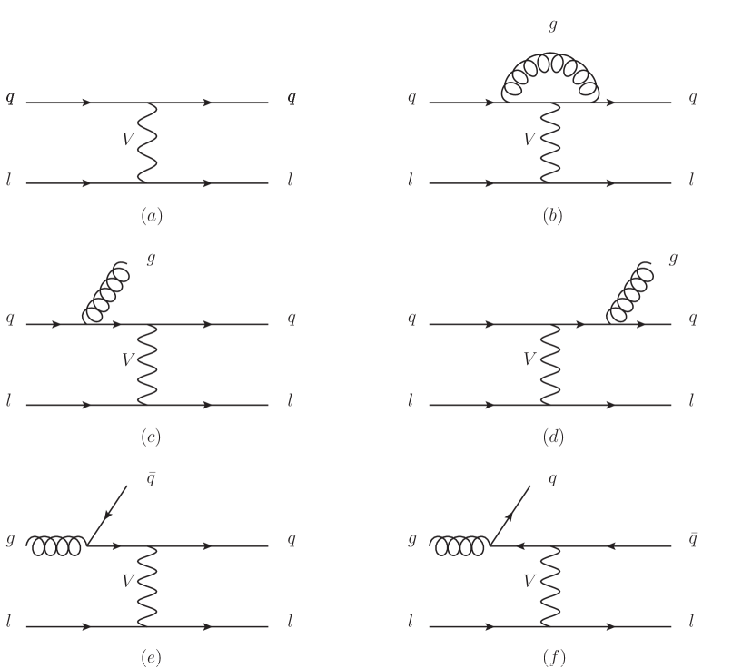
Figure 1: Feynman diagrams contributing to deep inelastic scattering at $\mathcal{O}(\alpha_{s})$: leading order (a), virtual (b) and real emission (c-f) corrections.

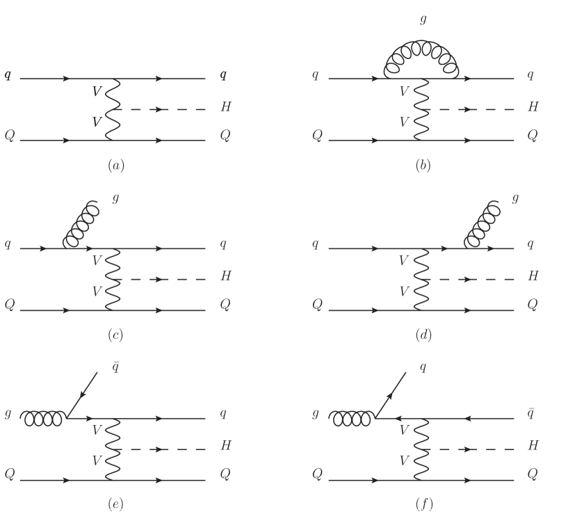
Figure 2: Feynman diagrams contributing to Higgs boson production via weak-boson fusion at $\mathcal{O}(\alpha_{s})$: leading order (a), virtual (b) and real emission (c-f) corrections. As matter of simplicity, we just show radiative corrections to the upper line in the gluon emission (c-d) and gluon initiated processes (e-f). In this case $V=W^{\pm}$ or $Z^{0}$.

At leading order DIS is described by the Feynman diagram shown in Fig. 1a, together with appropriate crossings of the quark line. The leading-order diagram for the VBF process is shown in Fig. 2a, together with appropriate crossings of the quark lines. In principle other contributions to the VBF process should be considered: diagrams with the exchange of identical outgoing quarks, the quark annihilation processes $\bar{q}q\to Z^{*}\to ZH$ and $\bar{q}q\to W^{\pm*}\to W^{\pm}H$ with hadronic decays of the vector bosons. However, colour suppression and the large momentum transfer in the weak-boson propagators make the contribution coming from these additional processes negligible in the phase-space regions where VBF can be observed experimentally, i.e. with widely separated quark jets of very large invariant mass [91].

At $\mathcal{O}(\alpha_{s})$, the contributions coming from amplitudes in which the gluon is attached to both upper and lower quark lines in the VBF process vanish because the weak boson has no colour charge. The Feynman graphs contributing are therefore only the ones shown in Figs. 2b-2f where for simplicity, we just show radiation from the upper quark line.

The corrections to the DIS and VBF processes are therefore the same provided that we take into account the corrections to both of the quark lines in the VBF process. In this section, we show the analytical contributions to the next-to-leading-order differential cross section for DIS and VBF. Collecting the real emission cross section, described in Sect. 3.1, virtual and collinear contributions, briefly discussed in Sect. 3.2, $\bar{B}(\Phi_{B})$ can be calculated. We then discuss how it is sampled within Herwig++ in Sect. 3.3.

3.1 Real emission contribution

The tree-level corrections to $e^{+}e^{-}$ annihilation to hadrons can be written in a form in which QCD and electroweak parts exactly factorize [92]. This method was later generalized to any process in which the lowest-order diagrams contain a single quark line attached to a single electroweak gauge boson [37]. We adopt this approach for the calculation of the real corrections to DIS and VBF, based on the calculation of the correction to DIS in Refs. [37, 33].

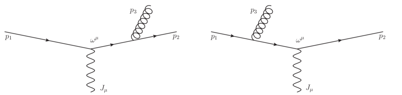
Figure 3: QCD Compton scattering, in which a quark interacts with an arbitrary current $J_{\mu}$ via boson-quark coupling $\omega^{\mu}$.

Consider the QCD Compton process, shown in Fig. 3, where a quark $q$ with momentum $p_{1}$ and a fraction $x_{B}$ of the incoming hadron momentum, interacts with a current $J_{\mu}$ and boson-parton coupling $\omega^{\mu}$, and scatters into an outgoing quark $q^{\prime}$ with momentum $p_{2}$ and a gluon with momentum $p_{3}$

$$\text{QCDC}:q(p_{1})+X\rightarrow q^{\prime}(p_{2})+g(p_{3})+X^{\prime}\text{.}$$ (4)

It is simplest to work in the Breit frame, in which the incoming parton for the leading-order process has four-momentum $q_{1}=\frac{Q}{2}(1;0,0,1)$, the exchanged boson has four-momentum $q=(0;0,0,-Q)$ and the scattered quark has four-momentum $q_{2}=\frac{Q}{2}(1;0,0,-1)$. In this frame the four-momenta of the real emission process are

$$p_{1} = \frac{Q}{2}(-x_{1};0,0,-x_{1});$$ (5a)

$$p_{2} = \frac{Q}{2}(\sqrt{x^{2}_{2}+x_{\perp}^{2}};\phantom{-}x_{\perp}\cos\phi,\phantom{-}x_{\perp}\sin\phi,-x_{2});$$ (5b)

$$p_{3} = \frac{Q}{2}(\sqrt{x^{2}_{3}+x_{\perp}^{2}};-x_{\perp}\cos\phi,-x_{\perp}\sin\phi,-x_{3});$$ (5c)

where the transfered momentum $q=(0;0,0,-Q)=p_{2}+p_{3}-p_{1}$ and

$$x_{i}=\frac{2p_{i}\cdot q}{q\cdot q}\text{.}$$ (6)

Momentum conservation requires that $x_{3}=2+x_{1}-x_{2}$ and

$$x_{\perp}^{2}=\frac{(x_{3}^{2}-x_{1}^{2}-x_{2}^{2})^{2}}{4x_{1}^{2}}-x^{2}_{2}.$$ (7)

In terms of these variables the cross section for the real emission process is

$${\rm d}\sigma_{\rm NLO}=\frac{1}{4(2\pi)^{2}}\frac{{\rm d}\phi}{2\pi}\frac{{\rm d}x_{1}{\rm d}x_{2}}{-x_{1}^{3}}\frac{-x_{1}x_{B}f(-x_{1}x_{B},Q^{2})}{x_{B}f(x_{B},Q^{2})}\frac{Q^{2}|\mathcal{M}_{\rm QCDC}|^{2}}{|\mathcal{M}_{\rm LO}(q_{1},q_{2})|^{2}}{\rm d}\sigma_{2},$$ (8)

where $x_{B}$ is the momentum fraction of the quark in the leading-order process, $|\mathcal{M}_{\rm QCDC}|^{2}$ and $|\mathcal{M}_{\rm LO}(q_{1},q_{2})|^{2}$ are the spin and colour averaged matrix elements squared for the real emission and leading-order processes respectively.

Using the gauge introduced by the CALKUL collaboration [93], the matrix element for the real emission process is [37, 33]

$$|\mathcal{M}_{\rm QCDC}|^{2}=-\frac{8\pi\alpha_{S}C_{F}}{(1+x_{1})(1-x_{2})Q^{2}}\left(x_{1}^{2}+(x_{2}^{2}+x_{\perp}^{2})R_{2}\right)|\mathcal{M}_{\rm LO}(q_{1},q_{2})|^{2},$$ (9)

where

$$R_{2}\equiv\frac{x_{2}^{2}}{x^{2}_{2}+x^{2}_{\perp}}\frac{|\mathcal{M}_{\rm LO}(\bar{r}_{1},r_{2})|^{2}}{|\mathcal{M}_{\rm LO}(q_{1},q_{2})|^{2}},$$ (10)

with $r_{2}=\frac{p_{2}}{x_{2}}$ and $\bar{r}_{1}=r_{2}-q$.

The integration of the phase space is simpler if we use the variables:

$$x_{1} = -\frac{1}{x_{p}};$$ (11a)

$$x_{2} = 1-\frac{1-z_{p}}{x_{p}};$$ (11b)

so that the phase-space limits become $x_{B}<x_{p}<1$ and $0<z_{p}<1$. In terms of these variables

$$x_{\perp}^{2}=\frac{4(1-x_{p})(1-z_{p})z_{p}}{x_{p}}\text{.}$$ (12)

The cross section for the real emission process becomes

$${\rm d}\sigma_{\rm NLO}=\frac{\alpha_{S}C_{F}}{2\pi}\frac{{\rm d}\phi}{2\pi}\frac{\frac{x_{B}}{x_{p}}f(\frac{x_{B}}{x_{p}},Q^{2})}{x_{B}f(x_{B},Q^{2})}\frac{{\rm d}x_{p}{\rm d}z_{p}}{(1-x_{p})(1-z_{p})}\left(1+x_{p}^{2}(x_{2}^{2}+x_{\perp}^{2})R_{2}\right){\rm d}\sigma_{2}.$$ (13)

This allows us to treat the QCD Compton process as a correction to the leading-order quark scattering process.

The boson-gluon fusion process,

$$\text{BGF}:g(p_{1})+X\rightarrow q^{\prime}(p_{2})+\bar{q}(p_{3})+X^{\prime}\text{,}$$ (14)

can be treated in a similar way. In this case the spin and colour averaged matrix element squared is

$$|\mathcal{M}_{\rm BGF}|^{2}=\frac{8\pi\alpha_{S}T_{R}}{(1-x_{2})(1-x_{3})Q^{2}}\left((x_{2}^{2}+x_{\perp}^{2})R_{2}+(x_{3}^{2}+x_{\perp}^{2})R_{3}\right),$$ (15)

where

$$R_{3}=\frac{x_{3}^{2}}{x_{3}^{2}+x_{\perp}^{2}}\frac{|\mathcal{M}_{\rm LO}(r_{3},r_{3}+q)|^{2}}{|\mathcal{M}_{\rm LO}(q_{1},q_{2})|^{2}}\text{,}$$ (16)

with $r_{3}=-p_{3}/x_{3}$.

Using the same change of variables as before the differential cross section is

$${\rm d}\sigma_{\rm NLO}=\frac{T_{R}\alpha_{S}}{2\pi}\frac{{\rm d}\phi}{2\pi}\frac{{\rm d}x_{p}{\rm d}z_{p}}{z_{p}(1-z_{p})}\frac{\frac{x_{B}}{x_{p}}f\left(\frac{x_{B}}{x_{p}},Q^{2}\right)}{x_{B}f(x_{B},Q^{2})}\left(x_{P}^{2}(x_{2}^{2}+x_{\perp}^{2})R_{2}+x_{P}^{2}(x_{3}^{2}+x_{\perp}^{2})R_{3}\right).$$ (17)

So far, our result gives the calculation of the BGF cross section, without any distinction between quark and antiquark scattering. If we want to view Eqn. 17 as a correction to a given lowest-order process, partons and antipartons should be treated equivalently. As the $z_{p}=1$ singularity is associated with configurations that become collinear to the lowest-order quark scattering process, while the $z_{p}=0$ singularity is associated with the antiquark scattering process, we can separate

$$\frac{1}{z_{p}(1-z_{p})}=\frac{1}{z_{p}}+\frac{1}{1-z_{p}}$$ (18)

and rewrite the cross section as

$${\rm d}\sigma_{\rm NLO}=\frac{T_{R}\alpha_{S}}{2\pi}\frac{{\rm d}\phi}{2\pi}\frac{{\rm d}x_{p}{\rm d}z_{p}}{(1-z_{p})}\frac{\frac{x_{B}}{x_{p}}f(\frac{x_{B}}{x_{p}})}{x_{B}f(x_{B})}\left(x_{P}^{2}(x_{2}^{2}+x_{\perp}^{2})R_{2}+x_{P}^{2}(x_{3}^{2}+x_{\perp}^{2})R_{3}\right),$$ (19)

with the corresponding $\frac{1}{z_{p}}$ term giving a correction to the antiquark scattering process [37, 33].

Using these results we can rewrite the real emission corrections as

$${\rm d}\sigma_{R}\equiv R(\Phi_{B},\Phi_{R})\mathrm{d}\Phi_{B}\mathrm{d}\Phi_{R},$$ (20)

where

$$R(\Phi_{B},\Phi_{R})=\sum_{I}R_{I}=B(\Phi_{B})\sum_{I}\frac{\mathcal{C}_{I}\alpha_{s}(\mu_{R})}{2\pi}\mathcal{A}_{I}\text{,}$$ (21)

with $I\in\left\{{\rm QCDC},{\rm BGF}\right\}$ and

$$\mathcal{C}_{\mathrm{QCDC}} = C_{F}\text{,}$$ (22a)

$$\mathcal{C}_{\mathrm{BGF}} = T_{R}\text{,}$$ (22b)

$$\mathcal{A}_{\mathrm{QCDC}} = \frac{\frac{x_{B}}{x_{p}}f_{q}(\frac{x_{B}}{x_{p}},Q^{2})}{x_{B}f_{q}(x_{B},Q^{2})}\frac{1}{(1-x_{p})(1-z_{p})}\left(1+x_{p}^{2}(x_{p}^{2}+x_{\perp}^{2}))R_{2}\right)\text{,}$$ (22c)

$$\mathcal{A}_{\mathrm{BGF}} = \frac{\frac{x_{B}}{x_{p}}f_{g}(\frac{x_{B}}{x_{p}},Q^{2})}{x_{B}f_{q}({x_{B},Q^{2})}}\frac{1}{(1-z_{p})}\left(x_{P}^{2}(x_{2}^{2}+x_{\perp}^{2})R_{2}+x_{P}^{2}(x_{3}^{2}+x_{\perp}^{2})R_{3}\right)\text{.}$$ (22d)

The radiative phase-space element is

$$\mathrm{d}\Phi_{R}=\frac{1}{2\pi}\mathrm{d}x_{p}\mathrm{d}z_{p}\mathrm{d}\phi\text{.}$$ (23)

The singularities in $R(\Phi_{B},\Phi_{R})$ are cancelled by subtracting

$$D_{I}=\frac{\mathcal{C}_{I}\alpha_{s}(\mu_{R})}{2\pi}\mathcal{D}_{I}\text{,}$$ (24)

where $\mathcal{D}_{I}$ are the Catani-Seymour dipoles [94]:

$$\mathcal{D}_{\mathrm{QCDC}} = \frac{\frac{x_{B}}{x_{p}}f_{g}(\frac{x_{B}}{x_{p}},Q^{2})}{x_{B}f_{q}(x_{B},Q^{2})}\frac{x_{p}^{2}+z_{p}^{2}}{(1-x_{p})(1-z_{p})}\text{;}$$ (25a)

$$\mathcal{D}_{\mathrm{BGF}} = \frac{\frac{x_{B}}{x_{p}}f_{g}(\frac{x_{B}}{x_{p}},Q^{2})}{x_{B}f_{q}(x_{B},Q^{2})}\frac{x_{p}^{2}+(1-x_{p})^{2}}{1-z_{p}}\text{.}$$ (25b)

The contribution of the real emission processes to $\bar{B}$ is therefore

$$B(\Phi_{B})\mathrm{d}\Phi_{B}\sum_{I\in\left\{{\rm QCDC},{\rm BGF}\right\}}\frac{\mathcal{C}_{I}\alpha_{s}(\mu_{R})}{2\pi}\left(\mathcal{A}_{I}-\mathcal{D}_{I}\right)\mathrm{d}\Phi_{R}\text{.}$$ (26)

While these expressions are sufficient for the calculation of the real correction, in the case of DIS the leading-order matrix elements are simple enough that $R_{2,3}$ can be calculated analytically and integrated over the azimuthal angle, $\phi$ and $z_{p}$ to simplify the numerical integration of $\bar{B}$.

For DIS [37, 33],

$$R_{2}=\frac{\cos^{2}\theta_{2}+\mathcal{A}\cos\theta_{2}\left(\ell-\sqrt{\ell^{2}-1}\sin\theta_{2}\cos\phi\right)+\left(\ell-\sqrt{\ell^{2}-1}\sin\theta_{2}\cos\phi\right)^{2}}{1+\mathcal{A}\ell+\ell^{2}},$$ (27)

where $\cos\theta_{2}=\frac{x_{2}}{\sqrt{x^{2}_{2}+x_{\perp}^{2}}}$, $\sin\theta_{3}=\frac{x_{\perp}}{\sqrt{x^{2}_{2}+x_{\perp}^{2}}}$, $\ell=\frac{2}{y_{B}}-1$, $y_{B}=\frac{q\cdot q_{1}}{p_{\ell}\cdot q_{1}}$ and $p_{\ell}$ is the four-momentum of the incoming lepton. $\mathcal{A}$ is related to the couplings of the fermions to the exchanged vector bosons. For the charged current process $\mathcal{A}=2$, whereas for the neutral current process

$$\mathcal{A}=\frac{4rC_{A,\ell}C_{A,q}\left(Q_{\ell}Q_{q}+2rC_{V,\ell}C_{V,q}\right)}{\left(Q_{\ell}^{2}Q_{q}^{2}+2Q_{\ell}Q_{q}rC_{V,\ell}C_{V,q}+r^{2}\left(C^{2}_{V,\ell}+C^{2}_{A,\ell}\right)\left(C^{2}_{V,q}+C^{2}_{A,q}\right)\right)},$$ (28)

with $r=\frac{Q^{2}}{(Q^{2}+m^{2}_{Z})}$ and

$$C_{V,i} = \frac{1}{\sin\theta_{W}\cos\theta_{W}}\left(\frac{I_{3,i}}{2}-Q_{i}\sin^{2}\theta_{W}\right)\text{,}$$ (29a)

$$C_{A,i} = \frac{1}{\sin\theta_{W}\cos\theta_{W}}\frac{I_{3,i}}{2},$$ (29b)

where $m_{Z}$ is the $Z^{0}$ boson mass, $\theta_{W}$ the Weinberg angle, $Q_{i}$ the fermion charge and $T_{3,i}$ its weak isospin.

The expression for $R_{3}$ can be obtained from that for $R_{2}$ with the exchange $\mathcal{}A\to-\mathcal{A}$, $\theta_{2}\to\theta_{3}$ and $\phi\to\pi-\phi$.

In this case the contribution to $\bar{B}$ is

$$B(\Phi_{B})\mathrm{d}\Phi_{B}{\rm d}x_{p}\sum_{I\in\left\{{\rm QCDC},{\rm BGF}\right\}}\frac{\alpha_{S}}{2\pi}S_{I},$$ (30)

where

$$S_{\rm QCDC} = \frac{\frac{x_{B}}{x_{p}}f_{q}(\frac{x_{B}}{x_{p}},Q^{2})}{x_{B}f_{q}(x_{B},Q^{2})}\frac{2+2\ell^{2}-x_{p}+3x_{p}\ell^{2}+\mathcal{A}\ell\left(1+2x_{p}\right)}{1+\mathcal{A}\ell+\ell^{2}},$$ (31a)

$$S_{\rm BGF} = -\frac{\frac{x_{B}}{x_{p}}f_{q}(\frac{x_{B}}{x_{p}},Q^{2})}{x_{B}f_{q}(x_{B},Q^{2})}\frac{1+\ell^{2}+2\left(1-3\ell^{2}\right)x_{p}(1-x_{p})+2\mathcal{A}\ell\left(1-2x_{p}(1-x_{p})\right)}{1+\mathcal{A}\ell+\ell^{2}}.$$

3.2 Virtual contribution and collinear remainders

The finite piece of the virtual correction is given by [91]

$$\mathrm{d}\sigma_{V}=\frac{C_{F}\alpha_{s}(\mu_{R})}{2\pi}V(x_{B})B(\Phi_{B})\text{,}$$ (32)

where the finite contribution of the $\mathbf{I}(\epsilon)$ operator of Ref. [94] and the virtual correction is

$$V(x_{B})=-\frac{\pi^{2}}{3}-\frac{9}{2}+\frac{3}{2}\ln\frac{Q^{2}}{\mu_{F}^{2}(1-x_{B})}+2\ln(1-x_{B})\ln\frac{Q^{2}}{\mu_{F}^{2}}+\ln^{2}(1-x_{B})\text{.}$$ (33)

The collinear remainders are

$$\mathrm{d}\sigma_{\rm coll}=\frac{C_{F}\alpha_{s}(\mu_{R})}{2\pi}\frac{f^{m}(x_{B},\mu_{F})}{f(x_{B},\mu_{F})}B(\Phi_{B})\text{,}$$ (34)

with the modified PDF

$$f^{m}_{q}(x_{B},\mu_{F}) = \int_{x_{B}}^{1}\frac{\mathrm{d}x_{p}}{x_{p}}\left\{f_{g}\left(\frac{x_{B}}{x_{p}},\mu_{F}\right)A(x_{p})\right.$$ (35)

$$+ \left.\left[f_{q}\left(\frac{x_{B}}{x_{p}},\mu_{F}\right)-x_{p}f_{q}(x_{B},\mu_{F})\right]B(x_{p})\right.$$

$$+ \left.f_{q}\left(\frac{x_{B}}{x_{p}},\mu_{F}\right)C(x_{p})\right\}\text{,}\ \ \$$

where $f_{q}$ and $f_{g}$ are the quark and gluon PDFs respectively, and

$$A(x_{p}) = \frac{T_{F}}{C_{F}}\left[x_{p}^{2}+(1-x_{p})^{2}\right]\mathrm{ln}\frac{Q^{2}(1-x_{p})}{\mu_{F}^{2}x_{p}}+2\frac{T_{F}}{C_{F}}x_{p}(1-x_{p})\text{,}$$ (36)

$$B(x_{p}) = \left[\frac{2}{1-x_{p}}\mathrm{ln}\frac{Q^{2}(1-x_{p})}{\mu_{F}^{2}}-\frac{3}{2}\frac{1}{1-x_{p}}\right]\text{,}$$ (37)

$$C(x_{p}) = \left[1-x_{p}-\frac{2}{1-x_{p}}\mathrm{ln}x_{p}-(1+x_{p})\mathrm{ln}\frac{Q^{2}(1-x_{p})}{\mu_{F}^{2}x_{p}}\right]\text{.}$$ (38)

The combined contribution of the finite virtual term and collinear remnants is

$$\mathrm{d}\sigma_{V+{\rm coll}}=\frac{C_{F}\alpha_{s}(\mu_{R})}{2\pi}\mathcal{V}(\Phi_{B})B(\Phi_{B})\text{,}$$ (39)

where

$$\mathcal{V}(\Phi_{B})\equiv V(x_{B})+\tilde{V}(x_{B},\mu_{F})\text{,}$$ (40)

with $\tilde{V}(x_{B},\mu_{F})=\frac{f^{m}(x_{B},\mu_{F})}{f(x_{B},\mu_{F})}$.

3.3 Sampling $\bar{B}$ within Herwig++

Using the results in the previous sections

$$\bar{B}(\Phi_{B}) = B(\Phi_{B})\left[1+\frac{C_{F}\alpha_{s}(\mu_{R})}{2\pi}\mathcal{V}(\Phi_{B})\right.$$ (41)

$$+ \left.\sum_{I\in\left\{{\rm QCDC},{\rm BGF}\right\}}\frac{\mathcal{C}_{I}\alpha_{s}(\mu_{R})}{2\pi}\int\left[\mathcal{A}_{I}(\Phi_{B},\Phi_{R})-\mathcal{D}_{I}(\Phi_{B},\Phi_{R})\right]\mathrm{d}\Phi_{R}\right]\text{.}$$

For convenience, the radiative variables $\left\{x_{p},z_{p},\phi\right\}$ are transformed into a new set $\left\{\tilde{x}_{p},z_{p},\tilde{\phi}\right\}$, defined on the interval $[0,1]$, such that the radiative phase space is a unit cube. The variable $x_{p}$ is redefined as

$$x_{p}=1-\rho^{\frac{1}{1-n}}\text{,}$$ (42)

where $n$ is fixed, and $\rho$ is the new variable with phase-space limits

$$0<\rho<(1-x_{B})^{1-n}\text{.}$$ (43)

This change of variable has been made in order to guarantee numerical stability in calculating the integral of $1/(1-x_{p})$. A further transformation is needed to achieve $\tilde{x}_{p}$:

$$\rho=(1-x_{B})^{1-n}\tilde{x}_{p}.$$ (44)

Finally, the variable $\phi$ is easily redefined as $\tilde{\phi}=\frac{\phi}{2\pi}$.

The sampling of $\bar{B}(\Phi_{B})$ proceeds in the following way:

1. generate a leading-order configuration using the standard Herwig++ leading-order matrix element generator, providing the Born variables $\Phi_{B}$ with an associated weight $B(\Phi_{B})$;

2. generate radiative variables, $\Phi_{R}$, by sampling $\bar{B}(\Phi_{B})$,which is parameterized in terms of the unit cube $(\tilde{x}_{p},z_{p},\tilde{\phi})$, and using the Auto-Compensating Divide-and-Conquer (ACDC) phase-space generator [95];

3. accepted the leading-order configuration with a probability proportional to the integrand of Eqn. 41 evaluated at $\left\{\Phi_{B},\Phi_{R}\right\}$.

In order to treat radiation from both quark lines in the VBF process we randomly select one line which emits the radiation and generate events in $\Phi\left\{\tilde{x}_{p},z_{p},\tilde{\phi}\right\}$. The symmetry of the process then ensures that the correct statistical result is obtained by multiplying the correction term in Eqn. 41 by two.

4 The generation of the hardest emission

The hardest emission is generated using the modified Sudakov form factor, given by the product of $\Delta_{R}(p_{T})$ for each channel contributing; this is done replacing the ratio $R(\Phi_{B},\Phi_{R})/B(\Phi_{B})$ in Eqn. 3 with

$$W_{I}(\Phi_{B},\Phi_{R})=\frac{{R}_{I}(\Phi_{B},\Phi_{R})}{B(\Phi_{B})}\text{.}$$ (45)

Moreover, we prefer to generate the hardest emission in terms of radiative variables $\Phi_{R}^{\prime}(x_{\perp},z_{p},\tilde{\phi})$ so that the $\theta$-function in Eqn. 3 simply gives $x_{\perp}$ as the upper limit of the integral and the modified Sudakov form factor, for the channel $I$, becomes

$$\Delta_{R_{I}}(x_{\perp})=\exp\left(-\int_{x_{\perp}}^{x_{\perp}^{\rm{max}}}\frac{{\rm d}x^{\prime}_{\perp}}{x^{\prime 3}_{\perp}}{\rm d}\tilde{\phi}{\rm d}z_{p}\frac{C_{I}\alpha_{S}}{2\pi}8z_{p}(1-z_{p})(1-x_{p})^{2}\mathcal{A}_{I}\right)\text{,}$$ (46)

where $\frac{Q}{2}x_{\perp}^{\rm{max}}$ is the maximum value for the transverse momentum.

The radiative variables are generated using the veto algorithm, described in [96]. We use the upper bounding function

$$g_{I}=\frac{a_{I}}{x_{\perp}^{3}}\text{,}$$ (47)

for the integrand which is chosen so that $g_{I}$ can be easily integrated in $\left\{x_{\perp},x_{\perp}^{\rm{max}}\right\}$. The generation procedure then proceeds as follows:

1. $x_{\perp}$ is set to $x_{\perp}^{\rm{max}}$;

2. a new $(\tilde{x}_{p},z_{p},\tilde{\phi})$ is randomly generated according to

   $$\Delta^{\rm over}_{R_{I}}(x_{\perp})=\exp\left(-\int_{x_{\perp}}^{x_{\perp}^{\rm{max}}}\frac{{\rm d}x^{\prime}_{\perp}}{x^{\prime 3}_{\perp}}{\rm d}\tilde{\phi}{\rm d}z_{p}a_{I}\right)\text{,}$$ (48)

   giving

   $$x_{\perp}^{2} = \frac{1}{\frac{1}{(x_{\perp}^{\rm{max}})^{2}}-\frac{2}{a_{I}}\ln{\mathcal{R}_{1}}}\text{,}$$ (49)

   $$z_{p} = \mathcal{R}_{2},$$ (50)

   $$\tilde{\phi} = \mathcal{R}_{3}.$$ (51)

3. if $\tilde{x}_{p}<0$ or $\tilde{x}_{p}>1$, the configuration generated is outside the phase-space boundaries, set $x^{\rm{max}}_{\perp}$ to $x_{\perp}$ and return to step 1;

4. if

   $$\frac{1}{g_{I}}\frac{C_{I}\alpha_{S}}{2\pi}8z_{p}(1-z_{p})(1-x_{p})^{2}\mathcal{A}_{I}>\mathcal{R},$$ (52)

   the configuration is accepted, otherwise set $x^{\rm{max}}_{\perp}$ to $x_{\perp}$ and return to step 1.

5 Truncated and vetoed parton showers

The Herwig++ shower algorithm, [97, 90], starts at an initial scale, given by the colour structure of the hard scattering process, and evolves down in the evolution variable related to the angular separation of parton branching products, $\tilde{q}$. The evolution is generated by the emission of partons in $1\to 2$ branching processes and each branching is described by a scale, $\tilde{q}$, a light-cone momentum fraction, $z$, and an azimuthal angle, $\phi$. The latter parameters are used to uniquely define the momenta of all particles radiated in a shower. However, the Herwig++ approach generally requires some reshuffling of these momenta after the generation of the parton showers to ensure global energy-momentum conservation.

($N+1$)-body final states associated to the generation of the hardest emission are first interpreted as a standard Herwig++ emission, from the $N$-body configuration, specified by the branching variables $(\tilde{q}_{h},z_{h},\phi_{h})$. The POWHEG emission is performed as a single Herwig++ shower as follows:

1. the truncated shower evolves from the default starting scale to $\tilde{q}_{h}$, such that any further emission conserves the flavour of the emitting parton and has transverse momentum lower than that of the hardest emission;

2. the hardest emission is forced with shower variables $(\tilde{q}_{h},z_{h},\phi_{h})$;

3. the vetoed shower evolves down to the hadronization scale, vetoing any emission with transverse momentum higher than that of the hardest emission.

The key feature of this approach is the ability to interpret the hard emission in terms of the shower variables. In order to do this we first need to consider the treatment of processes with an initial-state final-state colour connection, such as DIS or VBF, in the Herwig++ parton shower. In these processes the momenta of the incoming and outgoing colour connected partons after the parton shower are first reconstructed from the shower variables as described in Ref. [90]. These off-shell momenta are such that energy and momentum is not conserved, so boosts are applied to the incoming and outgoing momenta such that the momentum of the virtual boson is preserved by the showering process. In DIS and VBF type processes the reconstructed momenta are boosted to the Breit-frame of the system before the radiation. We take $p_{b}$ to be the momentum of the original incoming parton and $p_{c}$ to be the momentum of the original outgoing parton and $p_{a}=p_{c}-p_{b}$, therefore in the Breit-frame

$$p_{a}=Q(1;0,0,-1).$$ (53)

We can then construct a set of basis vectors,

$$n_{1} =Q(1;0,0,1), n_{2} =Q(1;0,0.-1).$$ (54)

The momenta of the off-shell incoming parton can be decomposed as

$$q_{\rm in}=\alpha_{\rm in}n_{1}+\beta_{\rm in}n_{2}+q_{\perp},$$ (55)

where $\alpha_{\rm in}=\frac{n_{2}\cdot q_{\rm in}}{n_{1}\cdot n_{2}}$, $\beta_{\rm in}=\frac{n_{1}\cdot q_{\rm in}}{n_{1}\cdot n_{2}}$ and $q_{\perp}=q_{\rm in}-\alpha_{\rm in}n_{1}-\beta_{\rm in}n_{2}$. In order to reconstruct the final-state momentum we first apply a rotation so that the momentum of the outgoing jet is

$$q_{\rm out}=\alpha_{\rm out}n_{1}+\beta_{\rm out}n_{2}+q_{\perp},$$ (56)

where $\beta_{\rm out}=1$ and the requirement that the virtual mass is preserved gives $\alpha_{\rm out}=\frac{q^{2}_{\rm out}+p^{2}_{\perp}}{2n_{1}\cdot n_{2}}$, with $q^{2}_{\perp}=-p^{2}_{\perp}$. The momenta of the jets are rescaled such that

$$q^{\prime}_{\rm in,out}=\alpha_{\rm in,out}k_{\rm in,out}n_{1}+\frac{\beta_{\rm in,out}}{k_{\rm in,out}}n_{2}+q_{\perp},$$ (57)

which ensures the virtual mass of the partons is preserved. The requirement that the momentum of the system is conserved, i.e.

$$p_{a}=q^{\prime}_{\rm out}-q^{\prime}_{\rm in}=Q(0,0,-1;0),$$ (58)

gives

$$\alpha_{\rm in}k_{\rm in}-\alpha_{\rm out}k_{\rm out} = \phantom{-}\frac{1}{2}\text{,}$$ (59a)

$$\frac{\beta_{\rm in}}{k_{\rm in}}-\frac{\beta_{\rm out}}{k_{\rm out}} = -\frac{1}{2}.$$ (59b)

Once the rescalings have been determined the jets are transformed using a boost such that

$$q_{\rm in,out}\stackrel{{\scriptstyle\mathrm{boost}}}{{\longrightarrow}}q_{\rm in,out}^{\prime}.$$ (60)

In order to interpret the hard emission in terms of the shower variables we first calculate the momentum of the off-shell incoming, $q^{\prime{\rm new}}_{b}$, or outgoing parton, $q^{\prime{\rm new}}_{c}$, depending on whether we are dealing with initial- or final-state radiation. We then compute the boost into the Breit-frame of this system and construct the basis vectors $n_{1,2}$ as before which allows us to determine the transverse momentum, $q_{\perp}$, of the off-shell incoming parton. In this frame the momenta of the partons before the shower would be:

$$p_{b} =\frac{Q}{2}(1+c;0,0,1+c); p_{c}=\frac{Q}{2}(1+c;0,0,-(1-c)).$$ (61)

The momenta of the off-shell partons before the boost required to conserve energy and momentum are

$$q_{b}^{\rm new} =\alpha^{\rm new}_{\rm in}n_{1}+\beta^{\rm new}_{\rm in}n_{2}+q_{\perp}\text{,} q_{c}^{\rm new} =\alpha^{\rm new}_{\rm out}n_{1}+\beta^{\rm new}_{\rm out}n_{2},$$ (62a)

where

$$\alpha^{\rm new}_{\rm in} =\frac{p_{b}\cdot n_{2}}{n_{1}\cdot n_{2}}, \beta^{\rm new}_{\rm in} =\frac{q_{b}^{\prime 2}-q^{2}_{\perp}}{2n_{1}\cdot n_{2}\alpha^{\rm new}_{\rm in}},$$ (63a)

$$\alpha^{\rm new}_{\rm out} =\frac{q_{c}^{\prime 2}}{2n_{1}\cdot n_{2}\beta^{\rm new}_{\rm out}}, \beta^{\rm new}_{\rm out} =\frac{p_{c}\cdot n_{1}}{n_{1}\cdot n_{2}}.$$ (63b)

The inverse of the boost, which would be applied in the shower to ensure energy-momentum conservation, can then be determined and applied to all the incoming and outgoing partons. These momenta can then be decomposed in terms of the Sudakov basis used in Herwig++, allowing the shower variables $(\tilde{q}_{h},z_{h},\phi_{h})$ to be determined.

6 Results

6.1 Deep Inelastic Scattering

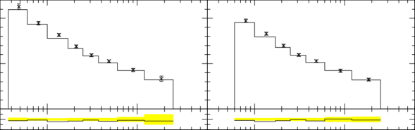
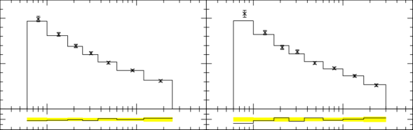
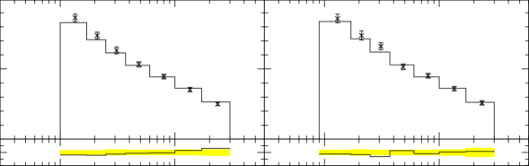
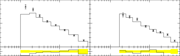
Figure 4: The $e^{+}p$ reduced cross section $\tilde{\sigma}^{e^{+}p}$, as a function of $x$ at fixed $Q^{2}$ between $200\,{\rm GeV}^{2}$ and $1500\,{\rm GeV}^{2}$. The experimental results of Ref. [98] are shown as crosses. The lower frame shows $({\rm Data}-{\rm Theory})/{\rm Data}$ and the yellow band gives the one sigma variation. The solid (black) line shows the Herwig++ result.

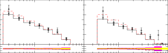
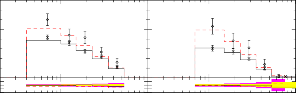
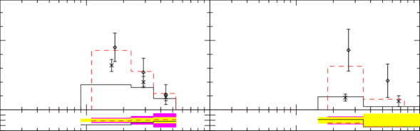
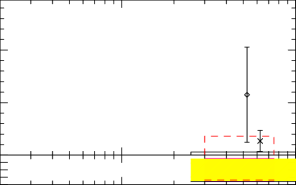
Figure 5: The $e^{\pm}p$ reduced cross section $\tilde{\sigma}^{e^{\pm}p}$, as a function of $x$ at fixed $Q^{2}$ between $200\,{\rm GeV}^{2}$ and $1500\,{\rm GeV}^{2}$. The experimental results of Ref. [98] for $\tilde{\sigma}^{e^{+}p}$ are shown as crosses and the results of Ref. [99] for $\tilde{\sigma}^{e^{-}p}$as diamonds. The lower frame shows $({\rm Data}-{\rm Theory})/{\rm Data}$ and the inner (yellow) band gives the one sigma variation for $\tilde{\sigma}^{e^{+}p}$ and the outer (magenta) band the one sigma variation for $\tilde{\sigma}^{e^{-}p}$. The solid (black) line shows the Herwig++ result for $\tilde{\sigma}^{e^{+}p}$ and the dashed (red) line shower the Herwig++ result for $\tilde{\sigma}^{e^{-}p}$.

In order to test our implementation of the POWHEG approach for deep inelastic scattering we first compared the results from Herwig++ and DISENT [100] for the reduced cross section

$$\tilde{\sigma}=\frac{xQ^{4}}{2\pi\alpha^{2}Y_{+}}\frac{{\rm d}^{2}\sigma}{{\rm d}x{\rm d}Q^{2}},$$ (64)

where $y=\frac{Q^{2}}{xs}$ and $Y_{\pm}\equiv 1\pm(1-y)^{2}$ and $\alpha$ is the fine-structure constant. The difference between the Herwig++ and DISENT results divided by the sum of the results is shown as a dashed line in the lower panels in Figs. 4 and 5 and is always less than one per mille. In addition Fig. 4 shows the comparison of the Herwig++ result with the results from Ref. [98] and Fig. 5 shows the comparison of the Herwig++ result with the results from Refs. [98] and [99]. The excellent agreement with DISENT and the experimental data demonstrates that the generation of the Born variables and calculation of $\bar{B}$ is correct. In both cases the PDFs from Ref. [101] were used.

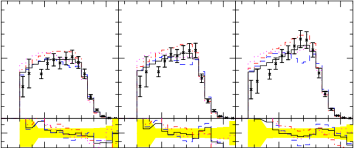
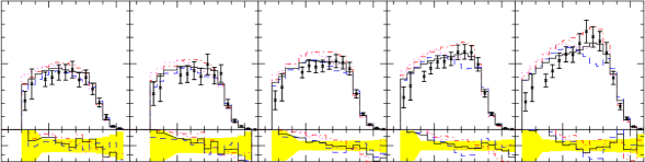
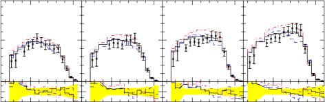
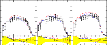
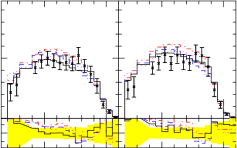
Figure 6: The inclusive transverse energy flow $\frac{1}{N}{\rm d}E_{T}^{*}/{\rm d}\eta^{*}$ at different values of $x$ and $Q^{2}$ for the low $Q^{2}$ sample from [102]. The lower frame shows $({\rm Data}-{\rm Theory})/{\rm Data}$ and the yellow band gives the one sigma variation.

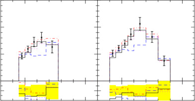
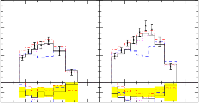
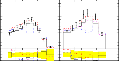
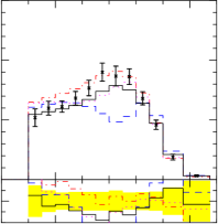
Figure 7: The inclusive transverse energy flow $\frac{1}{N}{\rm d}E_{T}^{*}/{\rm d}\eta^{*}$ at different values of $x$ and $Q^{2}$ for the high $Q^{2}$ sample from [102]. The lower frame shows $({\rm Data}-{\rm Theory})/{\rm Data}$ and the yellow band gives the one sigma variation.

In order to study the real emission we compare the results of Herwig++ with the measurements of the transverse energy flow in DIS from Ref. [102] which are sensitive to the treatment of hard radiation in angular-ordered parton showers [33]. The comparison of Herwig++ with the low and high $Q^{2}$ samples from Ref. [102] are shown in Figs. 6 and 7, respectively. In addition to the Herwig++ result, with and without the POWHEG correction, we have included the result of the FORTRAN HERWIG[31, 30] and Herwig++ with a matrix element correction based on the approach of Ref. [33]. These results clearly show that without a correction to describe hard QCD radiation there is a deficit of emissions between $1<\eta^{*}<3$ which is remedied by using either the POWHEG approach or a traditional matrix element correction. In general the POWHEG approach gives slightly less radiation than the matrix element due to the Sudakov suppression of radiation which is neglected in the matrix element correction approach and is in the best agreement with the experimental results. In these plots we have tuned the mass parameter for the splitting of soft beam remnant clusters in Herwig++ to 0.5 GeV from the HERWIG value of 1 GeV. The transverse energy flow in DIS is most sensitive to this parameter and the original HERWIG value was tuned to older transverse energy flow data.

6.2 Higgs Boson Production via Vector Boson Fusion

The typical feature of the VBF process at hadron colliders is the presence of two forward tagging jets. At leading order, they correspond to the two scattered quarks in the hard process and their observation, together with the properties of the Higgs boson decay products, is vital for the suppression of backgrounds [8, 9, 10, 11, 12, 13, 14]. The tagging jet distributions must be known precisely to gain a good estimate of the Higgs boson couplings: comparison of the Higgs boson production rate with the tagging jet cross section, within cuts, determines the Higgs boson couplings, [5, 6], and the uncertainties of the measured couplings are determined by the theoretical error of the cross section. At next-to-leading-order, the tagging jet distributions are sufficient to estimate size and uncertainties of the higher order QCD corrections, because the Higgs boson does not induce spin correlations in the phase space of its decay products.

A detailed analysis of jet distributions has been realized in the present work and the results are shown in this section. A preliminary step has been the validation of the $\bar{B}$ function, by comparing the NLO differential cross section as function of the rapidity of the stable Higgs boson given by Herwig++ and VBFNLO, as shown in Fig. 8.

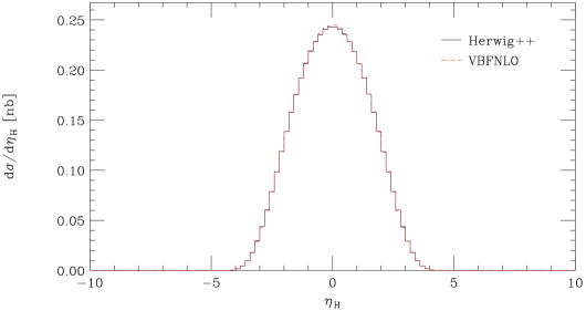
Figure 8: Rapidity of the Higgs boson at NLO. Results from Herwig++ (solid black line) are compared to the one from VBFNLO (dashed red line).

However, at next-to-leading-order we can either encounter two jets, with one of them composed of two partons (recombination effects), or three jets corresponding to well-separated partons. As for LHC data, an algorithm to select two tagging jets is needed. There are two possibilities [91]:

1. $p_{T}$-method: the two tagging jets are the two highest $p_{T}$ jets in the event;

2. $E$-method: the two tagging jets are the two highest energy jets in the event.

We follow the $p_{T}$-method and jets are defined according to the $k_{T}$ algorithm by using the FastJet package [103]. Cuts need to be chosen to reduce the effect of backgrounds and we follow the ones introduced in [91]. Tagging jets are required to have transverse momentum, $p_{T}$, and rapidity, $y_{j}$, fulfilling the following cuts:

$$p_{T}\geq 20~{}{\rm GeV}\text{,}\hskip 28.45274pt|y_{j}|\leq 4.5\text{.}$$ (65)

Moreover we generate the Higgs boson decay in $\tau^{+}\tau^{-}$ isotropically and require that the produced leptons have transverse momentum, $p_{T_{\tau^{(+,-)}}}$, and pseudorapidity, $\eta_{\tau^{(+,-)}}$, so that

$$p_{T_{\tau^{(+,-)}}}\geq 20~{}\rm{GeV}\text{,}\hskip 28.45274pt|\eta_{\tau^{(+,-)}}|\leq 2.5\text{.}$$ (66)

In addition, we require that jet-lepton separation in the rapidity-azimuthal angle plane satisfies

$$\Delta R_{j\tau^{(+,-)}}\geq 0.6\text{,}$$ (67)

and the tau leptons to lie between the two tagging jets in rapidity

$$y_{j,\rm{min}}<\eta_{\tau^{(+,-)}}<y_{j,{\rm{min}}}\text{.}$$ (68)

Backgrounds to VBF are significantly suppressed if the two tagging jets are well separated in rapidity; therefore, we require

$$|y_{j_{1}}-y_{j_{2}}|>4\text{.}$$ (69)

The factorization and the renormalization scale are chosen to be equal to the mass of the Higgs boson, $m_{H}=120~{}\rm{GeV}$. The other relevant electroweak parameters are

$$M_{W}=80.3980\rm{GeV}\text{,}\hskip 14.22636ptM_{Z}=91.1876\rm{GeV}\text{,}\hskip 14.22636pt\alpha_{em}=0.007556\text{,}\hskip 14.22636pt\rm{sin}^{2}\theta_{W}=0.222646\text{,}$$ (70)

and the weak coupling is computed as $g=\sqrt{4\alpha_{em}/\rm{sin}\theta_{W}}$. The parton distribution functions are chosen to be the CTEQ6M set [104, 105].

The analysis provides the comparison of distributions for POWHEG implementation (solid black curve) and LO simulation (dashed red curve) of Herwig++ parton shower together with VBFNLO NLO differential cross section (dotted blue curve).

In Fig. 9 we present the differential cross section as a function of the rapidity separation and higher $p_{T}$ of the two tagging jets. In the left panel we have excluded the cut in Eqn. 69. The cross sections show a peak at a rapidity of around $5$ in the left panel and a transverse momentum of $70$ GeV in the right panel. The POWHEG implementation leaves the cross section with respect to the $p_{T}$ of the hardest jet unchanged, while it modifies the difference of rapidity distribution respect to the LO simulation of the Herwig++ parton shower: the peak is slightly lower and shifted to a higher value of the rapidity difference.

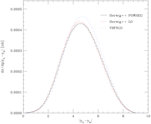
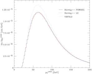
Figure 9: Difference of rapidity (left panel) and higher $p_{T}$ (right panel) distribution of the two tagging jets. In the left panel we have excluded the cut in Eqn. 69.

In Fig. 10 we plot the cross section with respect to the transverse momentum (left panel) and rapidity (right panel) of the softer of the two tagging jets. The transverse momentum distribution shows a peak around $30$ GeV and the rapidity around $2$. The Herwig++ shower provides a similar description at LO and NLO accuracy.

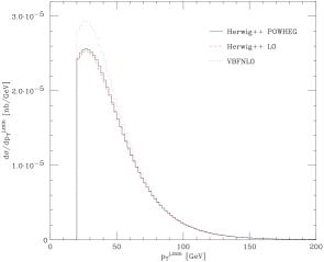
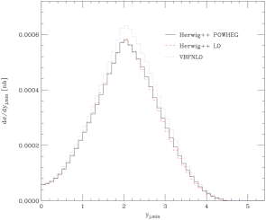
Figure 10: Distributions of smaller transverse momentum, $p_{T}^{j,{\rm min}}$, (left panel) and smaller rapidity, $y_{j,{\rm min}}$, (right panel) of the two tagging jets.

The transverse momentum and rapidity distributions of the third jet are plotted in Fig. 11 in the left and right panel respectively. As would be expected here we see a harder spectrum for the third jet in the POWHEG approach which is now simulated using the real emission matrix element rather than the shower approximation.

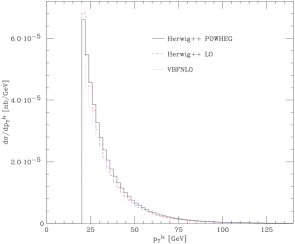
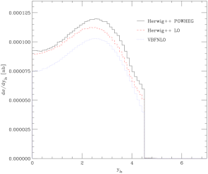
Figure 11: Transverse momentum distribution of the third jet ($p_{T}^{j_{3}}$) is plotted in the left panel and the rapidity distribution of the same jet ($y_{j_{3}}$) in the right one.

In these plots we see that the Herwig++ results lie below the fixed NLO results for distributions involving the two leading jets as a result of the subsequent parton shower, unlike the results of Ref. [75] where there is little difference between the POWHEG and fixed order results. This difference exists at both leading order and in the POWHEG approach in Herwig++ and is a result of the different shower algorithm and kinematic reconstruction in Herwig++. Given the excellent description of the related DIS data, compared with the previous HERWIG shower algorithm, this is an important difference in the two approaches and worthy of further study.

7 Conclusion

In this work the POWHEG NLO matching scheme has been implemented in the Herwig++ Monte Carlo event generator for DIS and Higgs boson production via vector boson fusion. For both hard subprocesses the $\bar{B}$ function has been calculated following the general approach provided in [36] which enables other colour-singlet VBF production processes to be easily included. The simulation contains a full treatment of the truncated shower, which is needed for the production of wide angle, soft radiation in angular-ordered parton showers.

For the DIS implementation we find the cross sections to be in good agreement with the experimental results of Refs.[98, 99, 102]. Our results show that the POWHEG approach correctly populates the so-called dead zone, as it appears in the transverse energy flow distributions at high $Q^{2}$.

For the VBF Higgs boson production we have shown different jet distributions after imposing typical cuts which are required to remove the effects of backgrounds. We find that the POWHEG implementation does improve the rapidity separation distribution for the two tagging jets and of $p_{T}$ and rapidity for the third hardest jet, while it mainly leaves the other distributions of the two tagging jets unchanged respect to the LO simulations within the Herwig++ parton shower.

The lack of data prevents us from comparing the jet distributions with experimental results. However, the present work together with the Higgs production via gluon fusion and the Higgs-strahlung simulations, which were already implemented in Herwig++ 2.3 [73], will provide an important tool for analyzing the upcoming results at the LHC.

References

- [1] F. Englert and R. Brout, Broken Symmetry and the mass of Gauge Vector Mesons, Phys. Rev. Lett. 13 (1964) 321–322.
- [2] P. W. Higgs, Broken Symmetries and the Masses of Gauge Bosons, Phys. Rev. Lett. 13 (1964) 508–509.
- [3] G. S. Guralnik, C. R. Hagen, and T. W. B. Kibble, Global Conservation Laws and Massless Particles, Phys. Rev. Lett. 13 (1964) 585–587.
- [4] T. W. B. Kibble, Symmetry breaking in non-Abelian gauge theories, Phys. Rev. 155 (1967) 1554–1561.
- [5] D. Zeppenfeld, R. Kinnunen, A. Nikitenko, and E. Richter-Was, Measuring Higgs boson couplings at the LHC, Phys. Rev. D62 (2000) 013009, [hep-ph/0002036].
- [6] A. Belyaev and L. Reina, , : toward a model independent determination of the Higgs boson couplings at the LHC, JHEP 08 (2002) 041, [hep-ph/0205270].
- [7] H. M. Georgi, S. L. Glashow, M. E. Machacek, and D. V. Nanopoulos, Higgs Bosons from Two Gluon Annihilation in Proton Proton Collisions, Phys. Rev. Lett. 40 (1978) 692.
- [8] D. L. Rainwater, D. Zeppenfeld, and K. Hagiwara, Searching for in weak boson fusion at the LHC, Phys. Rev. D59 (1999) 014037, [hep-ph/9808468].
- [9] T. Plehn, D. L. Rainwater, and D. Zeppenfeld, A method for identifying + missing at the CERN LHC, Phys. Rev. D61 (2000) 093005, [hep-ph/9911385].
- [10] D. L. Rainwater and D. Zeppenfeld, Observing in weak boson fusion with dual forward jet tagging at the CERN LHC, Phys. Rev. D60 (1999) 113004, [hep-ph/9906218].
- [11] N. Kauer, T. Plehn, D. L. Rainwater, and D. Zeppenfeld, as the discovery mode for a light Higgs boson, Phys. Lett. B503 (2001) 113–120, [hep-ph/0012351].
- [12] D. L. Rainwater and D. Zeppenfeld, Searching for in weak boson fusion at the LHC, JHEP 12 (1997) 005, [hep-ph/9712271].
- [13] O. J. P. Eboli and D. Zeppenfeld, Observing an invisible Higgs boson, Phys. Lett. B495 (2000) 147–154, [hep-ph/0009158].
- [14] D. Cavalli et. al., The Higgs working group: Summary report, hep-ph/0203056.
- [15] T. Han and S. Willenbrock, QCD correction to the p p W H and Z H total cross- sections, Phys. Lett. B273 (1991) 167–172.
- [16] A. Djouadi, M. Spira, and P. M. Zerwas, Production of Higgs bosons in proton colliders: QCD corrections, Phys. Lett. B264 (1991) 440–446.
- [17] M. Spira, A. Djouadi, D. Graudenz, and P. M. Zerwas, Higgs boson production at the LHC, Nucl. Phys. B453 (1995) 17–82, [hep-ph/9504378].
- [18] S. Dawson, Radiative corrections to Higgs boson production, Nucl. Phys. B359 (1991) 283–300.
- [19] W. Giele et. al., The QCD / SM working group: Summary report, hep-ph/0204316.
- [20] S. Catani, D. de Florian, and M. Grazzini, Higgs production in hadron collisions: Soft and virtual QCD corrections at NNLO, JHEP 05 (2001) 025, [hep-ph/0102227].
- [21] R. V. Harlander and W. B. Kilgore, Soft and virtual corrections to at NNLO, Phys. Rev. D64 (2001) 013015, [hep-ph/0102241].
- [22] R. V. Harlander and W. B. Kilgore, Next-to-next-to-leading order Higgs production at hadron colliders, Phys. Rev. Lett. 88 (2002) 201801, [hep-ph/0201206].
- [23] C. Anastasiou and K. Melnikov, Higgs boson production at hadron colliders in NNLO QCD, Nucl. Phys. B646 (2002) 220–256, [hep-ph/0207004].
- [24] V. Ravindran, J. Smith, and W. L. van Neerven, NNLO corrections to the total cross section for Higgs boson production in hadron hadron collisions, Nucl. Phys. B665 (2003) 325–366, [hep-ph/0302135].
- [25] A. Buckley et. al., General-purpose event generators for LHC physics, arXiv:1101.2599.
- [26] T. Sjostrand and M. Bengtsson, The Lund Monte Carlo for Jet Fragmentation and e+ e- Physics. Jetset Version 6.3: An Update, Comput. Phys. Commun. 43 (1987) 367.
- [27] M. Bengtsson and T. Sjostrand, Parton Showers in Leptoproduction Events, Z. Phys. C37 (1988) 465.
- [28] E. Norrbin and T. Sjostrand, QCD radiation off heavy particles, Nucl. Phys. B603 (2001) 297–342, [hep-ph/0010012].
- [29] G. Miu and T. Sjostrand, production in an improved parton shower approach, Phys. Lett. B449 (1999) 313–320, [hep-ph/9812455].
- [30] G. Corcella et. al., HERWIG 6: An event generator for Hadron Emission Reactions with Interfering Gluons (including supersymmetric processes), JHEP 01 (2001) 010, [hep-ph/0011363].
- [31] G. Corcella et. al., HERWIG 6.5 Release Note, hep-ph/0210213.
- [32] M. H. Seymour, Photon radiation in final state parton showering, Z. Phys. C56 (1992) 161–170.
- [33] M. H. Seymour, Matrix element corrections to parton shower simulation of deep inelastic scattering, . Contributed to 27th International Conference on High Energy Physics (ICHEP), Glasgow, Scotland, 20-27 Jul 1994.
- [34] G. Corcella and M. H. Seymour, Matrix element corrections to parton shower simulations of heavy quark decay, Phys. Lett. B442 (1998) 417–426, [hep-ph/9809451].
- [35] G. Corcella and M. H. Seymour, Initial state radiation in simulations of vector boson production at hadron colliders, Nucl. Phys. B565 (2000) 227–244, [hep-ph/9908388].
- [36] M. H. Seymour, Matrix Element Corrections to Parton Shower Algorithms, Comp. Phys. Commun. 90 (1995) 95–101, [hep-ph/9410414].
- [37] M. H. Seymour, A Simple prescription for first order corrections to quark scattering and annihilation processes, Nucl. Phys. B436 (1995) 443–460, [hep-ph/9410244].
- [38] S. Gieseke, A. Ribon, M. H. Seymour, P. Stephens, and B. Webber, Herwig++ 1.0: An Event Generator for Annihilation, JHEP 02 (2004) 005, [hep-ph/0311208].
- [39] S. Gieseke, The new Monte Carlo event generator Herwig++, hep-ph/0408034.
- [40] K. Hamilton and P. Richardson, A Simulation of QCD Radiation in Top Quark Decays, JHEP 02 (2007) 069, [hep-ph/0612236].
- [41] S. Gieseke et. al., Herwig++ 2.0 Release Note, hep-ph/0609306.
- [42] M. Bahr et. al., Herwig++ 2.2 Release Note, arXiv:0804.3053.
- [43] S. Gieseke, D. Grellscheid, K. Hamilton, A. Papaefstathiou, S. Platzer, et. al., Herwig++ 2.5 Release Note, arXiv:1102.1672.
- [44] S. Catani, F. Krauss, R. Kuhn, and B. R. Webber, QCD Matrix Elements + Parton Showers, JHEP 11 (2001) 063, [hep-ph/0109231].
- [45] F. Krauss, Matrix elements and parton showers in hadronic interactions, JHEP 08 (2002) 015, [hep-ph/0205283].
- [46] L. Lonnblad, Correcting the colour-dipole cascade model with fixed order matrix elements, JHEP 05 (2002) 046, [hep-ph/0112284].
- [47] A. Schalicke and F. Krauss, Implementing the ME+PS merging algorithm, JHEP 07 (2005) 018, [hep-ph/0503281].
- [48] F. Krauss, A. Schalicke, and G. Soff, APACIC++ 2.0: A Parton cascade in C++, Comput. Phys. Commun. 174 (2006) 876–902, [hep-ph/0503087].
- [49] N. Lavesson and L. Lonnblad, W + jets matrix elements and the dipole cascade, JHEP 07 (2005) 054, [hep-ph/0503293].
- [50] S. Mrenna and P. Richardson, Matching matrix elements and parton showers with HERWIG and PYTHIA, JHEP 05 (2004) 040, [hep-ph/0312274].
- [51] M. L. Mangano, M. Moretti, F. Piccinini, R. Pittau, and A. D. Polosa, ALPGEN, a generator for hard multiparton processes in hadronic collisions, JHEP 07 (2003) 001, [hep-ph/0206293].
- [52] J. Alwall et. al., Comparative study of various algorithms for the merging of parton showers and matrix elements in hadronic collisions, Eur. Phys. J. C53 (2008) 473–500, [arXiv:0706.2569].
- [53] S. Hoeche, F. Krauss, S. Schumann, and F. Siegert, QCD matrix elements and truncated showers, JHEP 05 (2009) 053, [arXiv:0903.1219].
- [54] K. Hamilton, P. Richardson, and J. Tully, A modified CKKW matrix element merging approach to angular-ordered parton showers, JHEP 11 (2009) 038, [arXiv:0905.3072].
- [55] S. Frixione and B. R. Webber, Matching NLO QCD Computations and Parton Shower Simulations, JHEP 06 (2002) 029, [hep-ph/0204244].
- [56] S. Frixione, F. Stoeckli, P. Torrielli, B. R. Webber, and C. D. White, The MC@NLO 4.0 Event Generator, arXiv:1010.0819.
- [57] S. Frixione, E. Laenen, P. Motylinski, and B. R. Webber, Single-top Production in MC@NLO, JHEP 03 (2006) 092, [hep-ph/0512250].
- [58] S. Frixione, E. Laenen, P. Motylinski, and B. R. Webber, Angular Correlations of Lepton Pairs from Vector Boson and Top Quark Decays in Monte Carlo Simulations, JHEP 04 (2007) 081, [hep-ph/0702198].
- [59] S. Frixione, E. Laenen, P. Motylinski, B. R. Webber, and C. D. White, Single-top hadroproduction in association with a W boson, JHEP 07 (2008) 029, [arXiv:0805.3067].
- [60] O. Latunde-Dada, Herwig++ Monte Carlo At Next-To-Leading Order for e+e- annihilation and lepton pair production, JHEP 11 (2007) 040, [arXiv:0708.4390].
- [61] O. Latunde-Dada, MC@NLO for the hadronic decay of Higgs bosons in associated production with vector bosons, JHEP 05 (2009) 112, [arXiv:0903.4135].
- [62] A. Papaefstathiou and O. Latunde-Dada, NLO production of bosons at hadron colliders using the MC@NLO and POWHEG methods, JHEP 07 (2009) 044, [arXiv:0901.3685].
- [63] P. Torrielli and S. Frixione, Matching NLO QCD computations with PYTHIA using MC@NLO, JHEP 1004 (2010) 110, [arXiv:1002.4293].
- [64] S. Frixione, F. Stoeckli, P. Torrielli, and B. R. Webber, NLO QCD corrections in Herwig++ with MC@NLO, JHEP 1101 (2011) 053, [arXiv:1010.0568].
- [65] P. Nason, A new method for combining NLO QCD with shower Monte Carlo algorithms, JHEP 11 (2004) 040, [hep-ph/0409146].
- [66] S. Frixione, P. Nason, and C. Oleari, Matching NLO QCD computations with Parton Shower simulations: the POWHEG method, JHEP 11 (2007) 070, [0709.2092].
- [67] P. Nason and G. Ridolfi, A Positive-Weight Next-to-leading-Order Monte Carlo for Z pair Hadroproduction, JHEP 08 (2006) 077, [hep-ph/0606275].
- [68] S. Frixione, P. Nason, and G. Ridolfi, A Positive-Weight Next-to-Leading-Order Monte Carlo for Heavy Flavour Hadroproduction, JHEP 09 (2007) 126, [arXiv:0707.3088].
- [69] O. Latunde-Dada, S. Gieseke, and B. Webber, A Positive-Weight Next-to-Leading-Order Monte Carlo for annihilation to hadrons, JHEP 02 (2007) 051, [hep-ph/0612281].
- [70] S. Alioli, P. Nason, C. Oleari, and E. Re, NLO vector-boson production matched with shower in POWHEG, JHEP 07 (2008) 060, [arXiv:0805.4802].
- [71] K. Hamilton, P. Richardson, and J. Tully, A Positive-Weight Next-to-Leading Order Monte Carlo Simulation of Drell-Yan Vector Boson Production, arXiv:0806.0290.
- [72] S. Alioli, P. Nason, C. Oleari, and E. Re, NLO Higgs boson production via gluon fusion matched with shower in POWHEG, JHEP 04 (2009) 002, [arXiv:0812.0578].
- [73] K. Hamilton, P. Richardson, and J. Tully, A Positive-Weight Next-to-Leading Order Monte Carlo Simulation for Higgs Boson Production, JHEP 04 (2009) 116, [arXiv:0903.4345].
- [74] S. Alioli, P. Nason, C. Oleari, and E. Re, NLO single-top production matched with shower in POWHEG: s- and t-channel contributions, JHEP 09 (2009) 111, [arXiv:0907.4076].
- [75] P. Nason and C. Oleari, NLO Higgs boson production via vector-boson fusion matched with shower in POWHEG, arXiv:0911.5299.
- [76] S. Hoche, F. Krauss, M. Schonherr, and F. Siegert, Automating the POWHEG method in Sherpa, JHEP 1104 (2011) 024, [arXiv:1008.5399].
- [77] S. Alioli, P. Nason, C. Oleari, and E. Re, A general framework for implementing NLO calculations in shower Monte Carlo programs: the POWHEG BOX, JHEP 1006 (2010) 043, [arXiv:1002.2581].
- [78] E. Re, Single-top production with the POWHEG method, PoS DIS2010 (2010) 172, [arXiv:1007.0498].
- [79] E. Re, Single-top Wt-channel production matched with parton showers using the POWHEG method, Eur.Phys.J. C71 (2011) 1547, [arXiv:1009.2450].
- [80] S. Alioli, P. Nason, C. Oleari, and E. Re, Vector boson plus one jet production in POWHEG, JHEP 1101 (2011) 095, [arXiv:1009.5594].
- [81] S. Alioli, K. Hamilton, P. Nason, C. Oleari, and E. Re, Jet pair production in POWHEG, JHEP 1104 (2011) 081, [arXiv:1012.3380].
- [82] K. Hamilton, A positive-weight next-to-leading order simulation of weak boson pair production, JHEP 01 (2011) 009, [arXiv:1009.5391].
- [83] C. Oleari, The POWHEG-BOX, Nucl.Phys.Proc.Suppl. 205-206 (2010) 36–41, [arXiv:1007.3893].
- [84] C. Oleari and L. Reina, W b bbar production in POWHEG, arXiv:1105.4488.
- [85] A. Kardos, C. Papadopoulos, and Z. Trocsanyi, Top quark pair production in association with a jet with NLO parton showering, arXiv:1101.2672.
- [86] T. Melia, P. Nason, R. Rontsch, and G. Zanderighi, plus dijet production in the POWHEGBOX, Eur. Phys. J. C71 (2011) 1670, [arXiv:1102.4846].
- [87] N. Lavesson and L. Lonnblad, Extending CKKW-merging to One-Loop Matrix Elements, JHEP 12 (2008) 070, [arXiv:0811.2912].
- [88] K. Hamilton and P. Nason, Improving NLO-parton shower matched simulations with higher order matrix elements, JHEP 06 (2010) 039, [arXiv:1004.1764].
- [89] S. Hoche, F. Krauss, M. Schonherr, and F. Siegert, NLO matrix elements and truncated showers, arXiv:1009.1127.
- [90] M. Bahr et. al., Herwig++ Physics and Manual, Eur. Phys. J. C58 (2008) 639–707, [arXiv:0803.0883].
- [91] T. Figy, C. Oleari, and D. Zeppenfeld, Next-to-leading order jet distributions for Higgs boson production via weak-boson fusion, Phys. Rev. D68 (2003) 073005, [hep-ph/0306109].
- [92] R. Kleiss, From two to three jets in heavy boson decays: An algorithmic approach, Phys. Lett. B180 (1986) 400.
- [93] P. De Causmaecker, R. Gastmans, W. Troost, and T. T. Wu, Multiple Bremsstrahlung in Gauge Theories at High- Energies. 1. General Formalism for Quantum Electrodynamics, Nucl. Phys. B206 (1982) 53.
- [94] S. Catani and M. H. Seymour, A general algorithm for calculating jet cross sections in NLO QCD, Nucl. Phys. B485 (1997) 291–419, [hep-ph/9605323].
- [95] L. Lönnblad, ThePEG, PYTHIA7, Herwig++ and ARIADNE, Nucl. Instrum. Meth. A559 (2006) 246–248.
- [96] T. Sjöstrand, S. Mrenna, and P. Skands, PYTHIA 6.4 Physics and Manual, JHEP 05 (2006) 026, [hep-ph/0603175].
- [97] S. Gieseke, P. Stephens, and B. Webber, New Formalism for QCD Parton Showers, JHEP 12 (2003) 045, [hep-ph/0310083].
- [98] ZEUS Collaboration, S. Chekanov et. al., High- neutral current cross sections in deep inelastic scattering at GeV, Phys. Rev. D70 (2004) 052001, [hep-ex/0401003].
- [99] ZEUS Collaboration, S. Chekanov et. al., Measurement of high- neutral current cross sections at HERA and the extraction of , Eur. Phys. J. C28 (2003) 175, [hep-ex/0208040].
- [100] S. Catani and M. H. Seymour, NLO QCD calculations in DIS at HERA based on the dipole formalism, hep-ph/9609521.
- [101] ZEUS Collaboration, S. Chekanov et. al., A ZEUS next-to-leading-order QCD analysis of data on deep inelastic scattering, Phys. Rev. D67 (2003) 012007, [hep-ex/0208023].
- [102] H1 Collaboration, C. Adloff et. al., Measurements of transverse energy flow in deep inelastic-scattering at HERA, Eur. Phys. J. C12 (2000) 595–607, [hep-ex/9907027].
- [103] M. Cacciari and G. P. Salam, Dispelling the myth for the jet-finder, Phys. Lett. B641 (2006) 57–61, [hep-ph/0512210].
- [104] J. Pumplin et. al., New generation of parton distributions with uncertainties from global QCD analysis, JHEP 07 (2002) 012, [hep-ph/0201195].
- [105] W.-K. Tung, New generation of parton distributions with uncertainties from global QCD analysis, Acta Phys. Polon. B33 (2002) 2933–2938, [hep-ph/0206114].