A macro-realism inequality for opto-electro-mechanical systems

Abstract

We show how to apply the Leggett-Garg inequality to opto-electro-mechanical systems near their quantum ground state. We find that by using a dichotomic quantum non-demolition measurement (via, e.g., an additional circuit-QED measurement device) either on the cavity or on the nano-mechanical system itself, the Leggett-Garg inequality is violated. We argue that only measurements on the mechanical system itself give a truly unambigous violation of the Leggett-Garg inequality for the mechanical system. In this case, a violation of the Leggett-Garg inequality indicates physics beyond that of “macroscopic realism” is occurring in the mechanical system. Finally, we discuss the difficulties in using unbound non-dichotomic observables with the Leggett-Garg inequality.

The Leggett-Garg (LG) inequality Leggett and Garg (1985); Leggett (2002); Korotkov (2001); Ruskov et al. (2006); Palacios-Laloy et al. (2009); Lambert et al. (2010a, b); Goggin et al. (2011) is one of a large class of inequalities used to delineate different physical theories. It is constructed to test for “macroscopic realism”, the class of physical theories that imply that before we measure a property of a system, that property has a well defined value (which is not the case in quantum mechanics). Bell’s inequality J. S. Bell (1964) also tested for this property, but not without also testing for non-locality. The LG inequality Leggett and Garg (1985); Leggett (2002) attempts to test only for realism, but to do so requires the assumption of non-invasive measurement, and macroscopically distinct states. Hence the moniker of “macroscopic realism”.

In the original LG proposal Leggett and Garg (1985), they imagined measuring the two different and distinct “macroscopic states” of a superconducting flux qubit (where, mathematically, one can describe these states as a quantum two-level system). However, physically these two states are by most definitions “macroscopic”: They involve millions of particles. Superconducting qubits have been used to show violations of Bell’s inequality  Ansmann et al. (2009), the Leggett-Garg inequality Palacios-Laloy et al. (2009), and have been proposed as a way to test the Kochen-Specker theorem Wei et al. (2010).

An alternative candidate to test for quantum behavior in the macroscopic limit is in the ground state of a nano-mechanical oscillator Cleland (2000); Blencowe (2005). Strong evidence has been reported of success in this goal by coupling a nanomechanical resonator to a qubit O’Connell et al. (2010) . Recent work suggests that the ground state has also been reached in an opto-mechanical device Teufel et al. (2011a, b). An opto-mechanical system is essentially an optical (or microwave) cavity coupled to a mechanical resonator to cool and measure the mechanical systemMetzger and Karrai (2004); Gigan et al. (2006). A generic physical model for this opto-mechanical system is of a spring that supports one of the mirrors of an optical cavity, and thus the mechanical motion of the spring is coupled to the frequency of the optical mode. However, the physical realization of opto-mechanical devices can vary greatly, from a mirror suspended on a cantilever Gigan et al. (2006), to a mechanical membrane capacitively coupled to a microwave transmission line Teufel et al. (2011a, b).

Reference Gigan et al. (2006) is an interesting example of the optical-cavity realization of an opto-mechanical system. They Gigan et al. (2006) showed side-band cooling from photo-pressure, and evidence of normal-mode splitting, i.e., strong coupling between optical and mechanical modes. Recent results Teufel et al. (2011a, b) using opto-electro-mechanical systems (i.e., a microwave transmission line in place of the optical cavity) have shown ultra-strong coupling and ground-state cooling. However one cannot easily distinguish the resultant effective low-temperature state of two coupled quantum oscillators from two coupled classical oscillators Wei et al. (2006); Xue et al. (2007). It is well known from quantum optics that the linear response spectral properties one observes are similar for both theories D.F Walls and G.J. Milburn (1995); Gigan et al. (2006); Clerk et al. (2010), though spectral properties can strongly infer cooling to the mechanical ground state Marquardt et al. (2007); Teufel et al. (2011a, b); Wei et al. (2006). In addition, the observation of asymmetry between spectral peaks due to absorption and emission of quanta is purely a quantum effect Clerk et al. (2010), and has been recently observed in experiment Safavi-Naeini et al. (2011).

In this work we propose a method of further distinguishing quantum and classical oscillators by applying the Leggett-Garg inequality. By using dichotomic quantum non-demolition measurements (QND)  Johnson et al. (2010); Schuster et al. (2007) we show that a theoretical model of a realistic opto-mechanical system implies a violation of the Leggett-Garg inequality due to the coherent interaction of the cavity with the mechanical oscillator. We show how either measurements on the cavity, or on the mechanical system directly, produce violations of the inequality. We argue that the latter are stronger proofs of quantum behaviour in the mechanical system, as the former can also occur due to the quantum nature of the cavity alone.

Since the dichotomic QND measurements we use here require strong coupling to a qubit our results are most directly applicable to opto-electro-mechanical systems which employ microwave transmission lines (as the “opto-electro-” cavity that cools the mechanical system to its quantum ground state). As far as we are aware, a dichotomic number state measurement has not been achieved in optical cavities. We believe the results we show here align well with Leggett and Garg’s original goal of testing for non-realism in the macroscopic world, since the ground state (or a single Fock state) of a mechanical oscillator represents a quantum state in a solid composed of millions of atoms.

We begin this article by outlining the original Leggett-Garg inequality, and discuss why dichotomic QND measurements are necessary. We then show our main result: that the introduction of a single photon into the microwave cavity, and application of dichotomic QND measurements, leads to a violation of the LG inequality. Afterwards we present the technical details of the model we use to describe the opto-electro-mechanical system, and discuss the practical issues of state preparation and measurement. We finish with a discussion of the difficulties of using non-dichotomic unbound measurements, and give a conjecture on a possible bound for the inequality in such a case.

I The Leggett-Garg inequality

The Leggett-Garg inequality Leggett and Garg (1985); Leggett (2002) is defined as follows: Given an observable $Q(t)$, which is bound above and below Korotkov (2001); Ruskov et al. (2006) by $|Q(t)|\leq 1$, the assumption of: (A1) macroscopic realism and (A2) non-invasive measurement implies,

$$L(t_{1},t_{2}) = \langle Q(t_{1})Q(0)\rangle+\langle Q(t_{1}\!+\!t_{2})Q(t_{1})\rangle$$ (1)

$$- \langle Q(t_{1}\!+\!t_{2})Q(0)\rangle\leq 1,\ \ \$$

If $Q$ is in the steady state at the initial time of measurement, and we set $t_{1}=t_{2}$, then this becomes

$$2\langle Q(\tau)Q(0)\rangle-\langle Q(2\tau)Q(0)\rangle\leq 1.$$ (2)

To adapt this to work on measurements on bosonic (harmonic) systems one must proceed with extreme caution. This is because (a) it is difficult to define a bound on measurements on harmonic systems, (b) many measurements (particularly in the optical regime) are invasive (e.g., single-photon counting) and (c) the dynamics of classical and quantum harmonic systems are identical (apart from quantum fluctuations) without additional sources of non-linearity.

Fortunately, the growing field of opto-electromechanical systems and circuit QED You and Nori (2003); Blais et al. (2004); You and Nori (2005, 2011); Buluta et al. (2011) allows us to overcome many of these obstacles. We can adapt the scheme realised by Johnson et al Johnson et al. (2010); Schuster et al. (2007) to overcome obstacle (a). In their scheme, one uses an additional qubit/measurement-cavity system to dispersively measure whether the optomechanical-cavity contains “one photon or not” (this is a dichotomic QND measurement). We will also show how, in principle, it might be possible to use this to measure the mechanical system directly, and say if it contains “one phonon or not”.

The former (a dichotomic QND measurement on the cavity) is possible due to the strong coupling between qubit and cavity that has been achieved in circuit-QED systems. The latter (a dichotomic QND measurement on the mechancical system) may be possible given the recent strong coupling shown between a mechanical system and a superconducting qubit O’Connell et al. (2010). A possible realization of the QND measurement on the cavity in an opto-electro-mechanical system is shown in Fig. 1.

This scheme also allows us to overcome obstacles (b) and (c), as it realizes a non-demolition, and classically non-invasive, projective measurement of the photons in the cavity (or phonons in the mechanical oscillator). In the final section we will return to these issues, and conjecture about a new bound for the inequality if one’s observables are non-dichotomic and unbound.

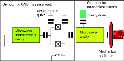
Figure 1: (Color online) Schematic diagram of a possible opto-electromechanical system with dichotomic QND measurement of the cavity. Right side of the figure: the driven microwave cavity is coupled to a mechanical oscillator, e.g. the fundamental mode of a thin film drum as in [Teufel et al., 2011a, b]. The left side of the figure shows a simplified schematic of the qubit/measurement-cavity system used for the dichotomic QND readout (as in Ref. [Johnson et al., 2010]). A similar measurement could be performed directly on the phonon states in the mechanical mode, given sufficiently strong coupling strengths between qubit and mechanical system (such a configuration is not shown in the figure).

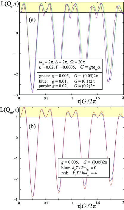
Figure 2: (Color online). Example of violation of Eq. (1) (with $t_{1}=t_{2}=\tau$) using (a) measurements on the cavity $Q_{c}$ and (b) measurements on the mechanical mode $Q_{m}$, as a function of the dimensionless time: $\tau|G|/2\pi$. Both figures are produced by our model of an opto-electromechanical system, where $G=g\omega_{m}\alpha$ is the effective coupling between the mechanical and cavity modes, and $\alpha\approx-\Omega/\Delta$ is the displacement of the cavity mode produced by the driving $\Omega$. For strong effective coupling, the non-energy conserving terms in our model begin to strongly modulate the shape of the correlation functions in Eq. (1). We have chosen ratios for the parameters that correspond approximately to those seen in the strong-driving limit of Ref. [Teufel et al., 2011a, b], where $\omega_{m}\approx 2\pi\times 10$ MHz, though to aid computation we made $g$ large, and $\Omega$ small, in comparison to their data. Remarkably, the high quality factor of both the microwave and mechanical cavities used in Teufel et al. (2011a, b) means that the violation of the inequality remains visible for relatively long time scales, though this can depend on the initial temperature of the mechanical mode.

II Violation for optomechanical systems using dichotomic QND measurements

We define the LG inequality in terms of dichotomic quantum non-demolition measurements either on the single-Fock state occupation of the cavity mode

$$Q_{c}=2|1\rangle_{c}\langle 1|_{c}-1,$$ (3)

where $c$ refers to the cavity mode, or on the single-phonon state occupation of the mechanical mode,

$$Q_{m}=2|1\rangle_{m}\langle 1|_{m}-1,$$ (4)

where $m$ refers to the mechanical mode. As mentioned above these measurements requires an additional qubit/measurement-cavity Johnson et al. (2010), which we outline in section IV, and is shown schematically in Fig. 1, for the example of measuring the cavity mode. For our purposes, this measurement returns $+1$ if there is a quanta in the appropriate mode ($m$ or $c$), and $-1$ if not. To show a violation of Eq. (1) one can prepare the opto-electromechanical system near its ground state following the side-band cooling procedure described in the next section. The ground state cooling of the mechanical system requires that we strongly drive the microwave cavity, resulting in a non-zero steady-state coherent occupation in the cavity in a rotating frame. Fortunately this can, in principle, be eliminated from the QND measurement (see section IV).

We then adiabatically introduce an additional photon into the cavity foo , in addition to this coherent state Johnson et al. (2010); Akram et al. (2010), which ideally prepares the system in the state

$$\rho(t=0)\ =\ |1\rangle_{c}\;\langle 1|_{c}\otimes|0\rangle_{m}\;\langle 0|_{m},$$ (5)

where again $c$ refers to the cavity and $m$ refers to the mechanical mode (note that the state of the cavity is in a displaced basis in a rotating frame because of the driving of the cavity). The strong coupling between the mechanical system and the optical mode causes this single excitation to be coherently exchanged (akin to a Rabi oscillation). One then measures the operator $Q_{c}$ (or $Q_{m}$) using the readout qubit-measurement-cavity and a programmable C-NOT scheme Johnson et al. (2010) (see section IV). If the measurement timescale (which includes rapidly resetting the qubit to its ground state) is short enough one can construct the two-time correlation functions in Eq. (1).

In Fig. 2 we explicitly show how the results from our model, outlined in the next section, which suggest a violation of Eq. (1), is in principle observable with existing experiments Teufel et al. (2011a, b); O’Connell et al. (2010). It is interesting to note that the largest violations occur for small times, which implies we require the readout and reset of the qubit to be fast. Typical readout times in Ref. [Johnson et al., 2010] are of the order of $550$ ns, introducing an intrinsic minimum delay into the correlation functions. The typical time scale of the coherent dynamics in Ref. [Teufel et al., 2011a, b] is related to the coupling, which is of the order of $10^{5}$–$10^{6}$ Hz, implying that the short time-scale coherent dynamics should be observable with such a measurement, though for measurements of $Q_{c}$ this may be altered by the need to measure in a rotating frame (see later). We also find that if the driving, and hence the coupling between cavity and mechanical system, is strong enough then the non-energy conserving terms in the interaction modulate the dynamics quite strongly. However at this point one also expects other non-linear affects to arise.

II.1 Ambiguities in cavity measurements

As we will discuss shortly, the measurement of $Q_{c}$ is a direct adaptation of an existing experiment (albeit with additional steps to make sure that we are measuring in the correct frame). However, our main goal is to verify the quantum dynamics of the mechanical mode. It just so happens that in this case it is the quantum coherent interaction between the cavity and mechanical modes which drives the violation we observe in the observables of the cavity system. However, in principle a violation could also be observed due to the quantum nature of the cavity mode alone.

Thus with measurements on the cavity mode alone it is impossible for us to state that a violation the Leggett-Garg inequality (e.g., with measurements $Q_{c}$) gives unambiguous proof of macroscopic quantum phenomena in the mechanical mode. Ideally, one requires dichotomic QND measurements on the mechanical mode directly (as defined by $Q_{m}$) to state that a violation of the Leggett-Garg inequality is unambiguous proof of quantum mechanics in the nano-mechanical system. We will outline a possible scheme to achieve this later.

III Optomechanical systems

We now explicitly describe the optomechanical system, and the model we use to calculate the results shown in Fig. 1. This model is well known and studied in other works Marquardt et al. (2007); Wilson-Rae et al. (2007), but we provide details here for clarity.

We start with the Hamiltonian describing the coupling between the cavity and the mechanical oscillator Law (1995),

$$H^{(1)} = \Delta a^{\dagger}a+\omega_{m}b^{\dagger}b+g\omega_{m}(b+b^{\dagger})a^{\dagger}a$$ (6)

$$+ \Omega(a+a^{\dagger})$$

The driving field is such that the cavity and mechanical mode are now near resonance ($\Delta=\omega_{m}$).

One of the approaches taken before (e.g.,  Marquardt et al. (2007); Wilson-Rae et al. (2007)) is to insert displacements $\alpha$ and $\beta$ for both modes, take the limit $g,g\alpha\ll\Delta,\omega_{m}$, and treat the cavity mode as an effective environment which cools the mechanical mode. The condition for cooling, in our notation, is then $\Delta>0$, and a sufficiently high-quality cavity $\kappa<\omega_{m}$. Reference  Gigan et al. (2006) has shown that by observing the homodyne transmission spectra from the (optical) cavity, we can see a clear signature of “normal mode splitting”. This is because the displacements $\alpha$ and $\beta$, and the coupling, are given by a simple model of two coupled oscillators, which has coupled normal modes. Here we explicitly model both cavity and mechanical system in the strong-coupling regime observed in Ref. [Teufel et al., 2011a] using a master equation approach.

III.1 Resolved side-band cooling

One can find the linearized version of the original Hamiltonian by displacing both mechanical and cavity modes, so that $a\rightarrow c+\alpha$, $b\rightarrow d+\beta$. Inserting these displacements in the Hamiltonian, and eliminating linear terms, gives two coupled equations for the displacements,

$$\alpha\Delta+2\omega_{m}g\alpha(\beta+\beta^{*})+\Omega-i\kappa=0$$ (7)

$$\omega_{m}\beta+\omega_{m}g\alpha^{2}=0$$ (8)

The $\kappa$ term arises because of the linear dissipation terms (cavity losses) we will introduce shortly. Careful inspection of the possible solutions of these cubic equations shows that,

$$\beta=-g\alpha\alpha^{*},$$ (9)

and in the limit of small $g$,

$$\alpha\approx\frac{-\Omega}{\Delta-i\kappa/2}.$$ (10)

If we do not make a small $g$ assumption, these displacements are real, up to some critical driving $\Omega$ of order $\omega_{m}/g$, which corresponds to the breakdown point of the small displacement assumption made to derive the original Hamiltonian (see Ref. [Law, 1995]). At this point additional non-linearities in the interaction could play a role, but we do not consider those here.

The Hamiltonian, with the linear terms eliminated, becomes

$$H^{(2)} = (\Delta+2g\omega_{m}\beta)c^{\dagger}c+\omega_{m}d^{\dagger}d$$

$$+ g\omega_{m}(d+d^{\dagger})(\alpha^{*}c+\alpha c^{\dagger})+g\omega_{m}(d+d^{\dagger})c^{\dagger}c.$$

We then add standard Lindblad cavity and mechanical losses to this model, and solve the resulting Master equation,

$$\dot{\rho} = -i[H^{(2)},\rho]$$

$$+ \frac{\kappa}{2}\left\{-c^{\dagger}c\rho-\rho c^{\dagger}c+2c\rho c^{\dagger}\right.$$

$$+ \left.\left[(\alpha^{*}c-\alpha c^{\dagger})\rho+\rho(\alpha c^{\dagger}-\alpha^{*}c)\right]\right\}$$

$$+ \frac{\Gamma}{2}(\bar{N}+1)\left[-d^{\dagger}d\rho-\rho d^{\dagger}d+2d\rho d^{\dagger}\right]$$

$$+ \frac{\Gamma}{2}\bar{N}\left[-dd^{\dagger}\rho-\rho dd^{\dagger}+2d^{\dagger}\rho d\right]$$

$$+ \frac{\Gamma}{2}\left[(\beta^{*}d-\beta d^{\dagger})\rho+\rho(\beta d^{\dagger}-\beta^{*}d)\right]$$

Where $\bar{N}$ is the initial thermal occupation of the mechanical mode. Dissipation terms linear in $c$ and $d$ (and displacements $\alpha$, $\beta$) arise because of the shifted coordinate frame. As mentioned earlier, the linear terms for the cavity can be easily eliminated by including them in the displacement $\alpha$. The linear terms for the mechanical mode dissipation are small in the limit of a high quality factor resonator, so we neglect them here (though we have numerically checked that their influence is small).

Under the conditions $\kappa<\omega_{m}$, $\Delta>0$ and sufficiently large driving strength $\Omega$, one can achieve the well-known resolved side-band-limit cooling; one can start from a thermal state of the resonator at a given temperature, and reach a steady-state, where the thermal phonon occupation of the mechanical system approaches zero. See Refs. [Marquardt et al., 2007; Wilson-Rae et al., 2007] for further details and discussion of the cooling process.

Using this model we can easily construct the various correlation functions needed for Eq. (1). Our technique is to prepare the system in the appropriate initial state; e.g. a single photon in the cavity (in the displaced basis)

$$\quad\rho(0)=|1_{c},0_{m}\rangle\langle 1_{c},0_{m}|,$$ (13)

then the appropriate correlation functions are calculated via the time evolution

$$\langle Q_{i}(2\tau)Q_{i}(\tau)\rangle=\mathrm{Tr}[Q_{i}\exp{[L\tau]}Q_{i}\exp{[L\tau]}\rho(0)],$$ (14)

or via the quantum regression theorem.

Since we operate always in the basis of the displaced modes, we are always close to the steady state. Thus imposing directly as initial conditions a single Fock state is a sufficiently good approximation to the true process of preparing the opto-mechanical system in its steady state, and then, e.g., introducing the single-photon state using the measurement qubit Johnson et al. (2010). In principle one can explicitly model this state-preparation stage Akram et al. (2010), but for simplicity we omit it here.

IV QND readout

As discussed earlier, both of these measurements, $Q_{c}$ and $Q_{m}$, are challenging, but may be feasible in the future by combining existing circuit-QED devices (for QND readout Johnson et al. (2010)) with an opto-electro-mechanical system Teufel et al. (2011a, b). The additional circuit-QED system (qubit and microwave cavity) allows both the deterministic preparation of the cavity in a single Fock state Liu et al. (2004); Hofheinz et al. (2007); Schuster et al. (2007); Hofheinz et al. (2008), and the dispersive QND readout of its population dynamics Johnson et al. (2010). Thus in reality our proposed opto-electro-mechanical system is a circuit-QED-mechanical system, where the additional qubit-cavity part is used for state preparation and readout. First of all we will describe the details (Fig. 1) of how to realize the measurement $Q_{c}$ (Ref. [Johnson et al., 2010]). As mentioned earlier, this is perhaps the most feasible with current technology, though does not give us an unambigous violation of the LG inequality for the mechanical mode. Then we will discuss possible ways that the measurement $Q_{m}$ might be realised by coupling the qubit directly to the mechanical system, and not the cavity, which give us a more ideal and unambigous violation of the LG inequality.

IV.1 Cavity measurement $Q_{c}$

The dichotomic QND measurement realized by Johnson et al [Johnson et al., 2010] is ideal for our purposes of realizing $Q_{c}$, but the scheme as it is described there Johnson et al. (2010) measures “if there is one cavity or not” in the lab basis. The cavity in the opto-mechanical Hamiltonian Eq. (6) we used earlier is in a displaced rotating frame (because of the microwave driving needed for sideband cooling), and thus it is in this basis that we must measure the cavity to realize $Q_{c}$ as we have described it. For example, in the stationary frame of the qubit (but rotating frame of the cavity), the interaction between qubit and cavity is described by,

$$H_{qb-c} = \frac{\epsilon}{2}\sigma_{z}+\Delta a^{\dagger}a+\lambda\left(\sigma_{+}ae^{-i\omega_{d}t}+\sigma_{-}a^{\dagger}e^{i\omega_{d}t}\right),$$

where $\omega_{d}$ is the driving frequency, and was chosen to bring the cavity and mechanical system on resonance in Eq. (6), so that

$$\Delta=\omega_{c}-\omega_{d}\approx\omega_{m}.$$ (16)

In addition, we also displace the cavity co-ordinates by $\alpha$, so that the interaction between the qubit and cavity co-ordinates that we actually want to measure is

$$\bar{H}_{qb-c} = \frac{\epsilon}{2}\sigma_{z}+\Delta c^{\dagger}c+\lambda\left(\sigma_{+}ce^{-i\omega_{d}t}+\sigma_{-}c^{\dagger}e^{i\omega_{d}t}\right)$$ (17)

$$+ \lambda\left(\alpha e^{-i\omega_{d}t}\sigma_{+}+\alpha^{*}e^{i\omega_{d}t}\sigma_{-}\right),$$

The additional displacement term represents the large number of photons that are in the cavity due to the driving. Ideally their influence on the qubit can be eliminated by applying an additional microwave drive to the qubit itself Blais et al. (2004) (still in the lab frame), out of phase with the term above, e.g.,

$$H_{\mathrm{adjust}}=-\lambda\left(\alpha e^{-i\omega_{d}t}\sigma_{+}+\alpha^{*}e^{i\omega_{d}t}\sigma_{-}\right).$$ (18)

This is feasible if the magnitude, $\lambda\alpha$, is not too large Blais et al. (2004), but may become unfeasible if an extremely large driving of the cavity is needed for cooling.

Assuming this term has been applied, and the effect of the large cavity population eliminated, we can move the qubit into the same frame as the cavity with the unitary transformation $U_{q}=\exp\left(i\omega_{d}\sigma_{z}t/2\right)$. This leaves us with a normal Jaynes-Cummings Hamiltonian between qubit and cavity, with a shifted qubit energy

$$\Delta^{\prime}=\epsilon-\omega_{d}.$$ (19)

In this new picture, the QND measurement scheme proposed and analyzed elsewhere Blais et al. (2004); Clerk and Utami (2007); Johnson et al. (2010) applies for a large bias

$$\delta=\Delta^{\prime}-\Delta=\epsilon-\omega_{c}.$$ (20)

This is clearly shown by applying the unitary transformation $U_{d}HU_{d}^{\dagger}$, $U_{d}=\exp{\left[\frac{\lambda}{\delta}(c\sigma_{+}-c^{\dagger}\sigma_{-})\right]}$, which leads to the well-known dispersive coupling Hamiltonian (see, e.g., Refs. [Blais et al., 2004; Clerk and Utami, 2007]),

$$H_{qb-D} = \left[\frac{\Delta^{\prime}}{2}+\frac{\lambda^{2}}{\delta}\left(c^{\dagger}c+\frac{1}{2}\right)\right]\sigma_{z}+\Delta c^{\dagger}c.$$ (21)

This transformation can induce interactions between the measurement qubit and the mechanical mode, but these terms can also be treated with a dispersive transformation, and give a shift of the qubit frequency of order $(\lambda g\alpha\omega_{m})^{2}/\delta^{3}$, and are thus much weaker than the $\lambda^{2}/\delta$ shift. In addition, the higher-order terms in $\lambda/\delta$ (representing back-action of the qubit on the cavity) should be much smaller than the cavity-mechanical mode interaction (i.e., $\lambda^{3}/\delta^{2}\ll g\alpha\omega_{m}$).

In Ref. [Johnson et al., 2010], in order to have sufficiently high resolution measurement of the effect of the photons on the energy levels of the qubit, they needed $\delta/\lambda<10$. That is, they need sufficiently large $\delta$ to reach the dispersive limit, but sufficiently strong $\lambda$ to obtain well resolved energy shifts for different photon occupations. Here, $\delta==\epsilon-\omega_{c}$, thus reaching the same regime as $\delta/\lambda<10$ seems feasible.

The dichotomic property of the measurement is achieved because of the strong dependence of the qubit response on the number of photons in the cavity. In Ref. [Johnson et al., 2010], for the measurement step, they apply a $\pi$ control pulse to the qubit at the frequency corresponding to its energy when just one photon is in the cavity. Thus the qubit is rotated if and only if there is one photon present, and nothing happens otherwise. This is an effective CNOT gate on the qubit and the cavity. Here, the effective CNOT gate must also be in the rotating frame of the qubit. For the final measurement step, one measures the state of the qubit via pulsed spectroscopy of the cavity.

Overall, this dispersive Hamiltonian, combined with the controlled-$\pi$-rotation of the qubit, and readout of the qubit using the additional measurement cavity (which we have not explicitly described), ideally gives us a way to realize the dichotomic QND measurement $Q_{c}=2|1\rangle_{c}\langle 1|_{c}-1$. As we discussed earlier, the time needed in Ref. [Johnson et al., 2010] to realize this measurement may be short enough to observe correlation functions on the time scale we require. However, in general there will be losses involved in the measurement process (e.g., due to dissipation of the qubit state) which will degrade the measurement result Johnson et al. (2010). In addition, the need to perform the effective CNOT gate in the rotating frame may slow down the measurement step Blais et al. (2004).

IV.2 Mechanical measurement $Q_{m}$

As we have reiterated several times, a measurement of $Q_{c}$ is not sufficient to unambiguously show quantum dynamics in the mechanical mode. We ideally need to perform the dichotomic QND measurement on the mechanical system itself. As far as we are aware no similar measurement has yet been achieved, though efforts on membrane-in-the-middle devices Clerk et al. (2010) are promising. Staying within the regime of the nano-mechanical systems we have discussed so far Teufel et al. (2011a, b); O’Connell et al. (2010), one can imagine adapting the scheme of Johnson et al [Johnson et al., 2010] to directly measure the mechanical mode. In Ref. [O’Connell et al., 2010] O’Connell et al observed a strong interaction between a high-frequency mechanical mode and a superconducting qubit. There the mechanical mode frequency was $\omega_{m}/2\pi=6$ GHz, so cryogenic freezing was sufficient to reach the quantum ground state, and they observed qubit-oscillator coupling strengths of $\lambda/h=110$ MHz. This is favorable for using the qubit as a dispersive measurement of the mechanical mode. However a straight adaptation of Ref. [Johnson et al., 2010] to the system in Ref. [O’Connell et al., 2010] would have to compensate for the extremely short quality factor of the mechanical resonator (the mechanical dephasing time is estimated to be $T\approx 20$ ns). This is well short of the measurement time in Ref. [Johnson et al., 2010], and thus resolving the short time correlations needed to see a violation of the inequality may prove difficult without improvements in the readout and reset times of the qubit, or employing a higher quality factor/lower frequency mechanical resonator.

Furthermore, one can imagine a similar scenario using the opto-mechanical side-band cooling systems we have described here, where the low frequency (and high quality factor) mechanical system is cooled by the cavity, and then the mechanical part is measured in the same manner as above (by an additional superconducting qubit, with compensation for the coherent occupation $\beta$). This is quite a speculative scenario, as it is not clear if a sufficiently large coupling between the qubit and the type of mechanical oscillator used in opto-electro-mechanical devices  Teufel et al. (2011a, b) can be engineered, and if the overly large energy mismatch between the superconducting qubit and mechanical resonator overcome. However if realised it would be ideal for truly showing macroscopic quantum phenomena in the same spirit as Leggett and Garg’s proposal Leggett and Garg (1985).

IV.3 Single photon measurements

For the optical-cavity realization of an optomechancial system (as in Ref. Gigan et al. (2006)), the Fock state preparation (e.g., by using an additional one-way cavity as discussed in Ref. [Akram et al., 2010]), and QND measurements Guerlin et al. (2007), are feasible but the dichotomic measurements we require are much more difficult to realise than in the microwave cavity case.

We also point out that the correlators in Eq. (1) are not normal ordered, and thus do not represent the measurements obtained from single-photon counting (which are typical in optical cavity systems). As we discussed in earlier work Lambert et al. (2010a, b), photon absorbtion measurements are fundamentally invasive, and typically represent an obstacle for un-conditionally verifying quantum behavior via the Leggett-Garg inequality. This is particularly true with a fragile single-quantum Fock state, hence the need for QND measurements.

V Non-dichotomic and unbound observables

What happens if we attempt to construct the Leggett-Garg inequality from non-dichotomic and unbound observables? Recent work on Bell’s inequality with unbound measurements Bednorz and Belzig (2011); Bednorz et al. (2011) suggest that one has to move to fourth-order correlation functions to distinguish quantum and classical correlations, which may also apply to the Leggett-Garg inequality.

First of all, let us consider a general picture where we measure an unbound operator $\langle\hat{Q}\rangle\in\{-\infty,\infty\}$. Following the same reasoning as used in the Leggett-Garg inequality one can derive a bound (and assuming we construct our expectation values by counting how often a particular measurement result arises),

$$L_{Q}\leq\langle\mathrm{Max}_{t}[Q(t)]^{2}\rangle.$$ (22)

Such a bound may occur due to some intrinsic conservation rule in the system (e.g., if the number state or energy is conserved). However, this bound is both difficult to calculate (and measure) and is extremely loose, since in general extremum values may be observed but contribute little to the expectation values. Since the maximization is a convex function, we know that

$$\mathrm{Max}_{t}[\langle Q(t)^{2}\rangle]\leq\langle\mathrm{Max}_{t}[Q(t)]^{2}\rangle,$$ (23)

(this is the Jensen inequality), but finding further constraints on these functions is challenging beyond trivial cases. We conjecture that there might be a tighter bound for the inequality given by $\mathrm{Max}_{t}[\langle Q(t)^{2}\rangle]$. However we have been unable to find a rigorous proof, and it may be that a simple counter-example exists to show that this conjecture does not hold.

There is a further caveat on such an approach. Note that taking the stationary limit and setting ($t_{1}=t_{2}=\tau$) simplifies the inequality with our conjectured bound $\mathrm{Max}_{t}[\langle Q(t)^{2}\rangle]$ to, $L_{Q}^{(2)}=2\langle Q(\tau)Q(0)\rangle-\langle Q(2\tau)Q(0)\rangle\leq\langle Q(0)^{2}\rangle.$ In a classical situation, the correlation functions one can observe are harmonic functions (even in the stationary state). For example, one can easily solve the equation of motion for a single oscillator in contact with a thermal bath, and find that the spectral density of the displacement Cleland (2000) is a Lorentzian with amplitude $\frac{2k_{B}T}{\pi mQ}$ related to the bath temperature $T$. The Wiener-Khinchin theorem tells us that the spectral density is the Fourier transform of the auto-correlation function in the steady state, implying sinusoidal correlation functions which are only dependent on one time variable (the time between measurements). These obviously cause a violation of the bound $\langle Q(0)^{2}\rangle$ in the steady state. One can argue that this is not per se a failure of our conjectured bound, but is because the only output one observes from the system is noise-driven; the thermal background has a white noise spectrum, which can thus excite the system around its resonant frequency. Thus, in the language of Leggett-Garg, these classical correlation functions are essentially invasive since one only observes a signal when the system fluctuates (e.g., due to thermal fluctuations). Therefore, the observation of thermal-noise-induced fluctuations is equivalent to a perturbation of the system by the measurement.

The original Leggett-Garg inequality avoids this problem by demanding that the system must be in one of two macroscopically distinct states, and that the system is almost always in one of the two states Leggett and Garg (1985); Leggett (2002). In a harmonic system this assumption, of macroscopically distinct states, breaks down spectacularly. One can overcome this problem by avoiding the steady state, or introducing a third measurement (if $Q\in\{0,\infty\}$, or a third and fourth measurement if $Q\in\{-\infty,\infty\}$) into all correlation functions in the inequality at time $t=0$, and scaling the bound appropriately. Then the violation is dependent on the effect of the second measurement (which we assume again to be non-invasive). The quasi-invasive (fluctuation) nature of the first measurement becomes irrelevant. Introducing extra measurements into the inequality is akin to the fourth-order Bell inequality derived by Bednorz et al Bednorz and Belzig (2011); Bednorz et al. (2011). However more work remains to be done to derive rigorous proofs for our conjecture.

VI Conclusions

In summary, we discussed how to use the Leggett-Garg inequality to distinguish quantum and classical dynamics in opto-electro-mechanical systems. We illustrated that dichotomic QND measurements of either the cavity or mechanical system leads to a violation of this inequality. We discussed possible methods to realize such measurements, and argued that only measurements directly on the mechanical system itself will give unambigous proof of macroscopic quantum dynamics in the mechanical system (or, in the language of Leggett and Garg, proof of a violation of macroscopic realism).

VII Acknowledgments

We thank T. Brandes, C. Emary, S. De Liberato and I. Mahboob for useful discussions. NL is supported by the RIKEN FPR program. JR is supported the Japanese Society for the Promotion of Science (JSPS). FN acknowledges partial support from the Laboratory of Physical Sciences, National Security Agency, Army Research Office, Defense Advanced Research Projects Agency, Air Force Office of Scientific Research, National Science Foundation Grant No. 0726909, JSPS-RFBR Contract No. 09-02-92114, Grant-in-Aid for Scientific Research (S), MEXT Kakenhi on Quantum Cybernetics, and the JSPS via its FIRST program.

References

- Leggett and Garg (1985) A. J. Leggett and A. Garg, Phys. Rev. Lett 54, 857 (1985).
- Leggett (2002) A. J. Leggett, J. Phys.: Condens. Matter 14, R415 (2002).
- Korotkov (2001) A. N. Korotkov, Phys. Rev. B 63, 085312 (2001).
- Ruskov et al. (2006) R. Ruskov, A. N. Korotkov, and A. Mizel, Phys. Rev. Lett 96, 200404 (2006).
- Palacios-Laloy et al. (2009) A. Palacios-Laloy, F. Mallet, F. Nguyen, P. Bertet, D. Vion, D. Esteve, and A. Korotkov, Nature Physics, 6, 442 (2009).
- Lambert et al. (2010a) N. Lambert, C. Emary, Y.-N. Chen, and F. Nori, Phys. Rev. Lett. 105, 176801 (2010a).
- Lambert et al. (2010b) N. Lambert, Y.-N. Chen, and F. Nori, Phys. Rev. A. 82, 063840 (2010b).
- Goggin et al. (2011) M. E. Goggin, M. P. Almeida, M. Barbieri, B. P. Lanyon, J. L. O’Brien, A. G. White, and G. J. Pryde, Proc. Natl. Acad. Sci. 108, 1256 (2011).
- J. S. Bell (1964) J. S. Bell, Physics 1, 195 (1964).
- Ansmann et al. (2009) M. Ansmann et al., Nature 461, 504 (2009).
- Wei et al. (2010) L. F. Wei, K. Maruyama, X.-B. Wang, J. Q. You, and F. Nori, Phys. Rev. B 81, 174513 (2010).
- Cleland (2000) A. N. Cleland, Foundations of Nanomechanics (Springer, Heidelberg, 2000).
- Blencowe (2005) M. Blencowe, Contemporary Phys. 46, 249 (2005).
- O’Connell et al. (2010) A. D. O’Connell et al., Nature 464, 697 (2010).
- Teufel et al. (2011a) J. D. Teufel, D. Li, M. S. Allman, K. Cicak, A. J. Sirois, J. D. Whittaker, and R. W. Simmonds, Nature 471, 204 (2011a).
- Teufel et al. (2011b) J. D. Teufel et al., arxiv:1103.2144v1 (2011b).
- Metzger and Karrai (2004) C. Metzger and K. Karrai, Nature 432, 1002 (2004).
- Gigan et al. (2006) S. Gigan et al., Nature 444, 67 (2006).
- Wei et al. (2006) L. F. Wei, Y. X. Liu, C. P. Sun, and F. Nori, Phys. Rev. Lett. 97, 237201 (2006).
- Xue et al. (2007) F. Xue, Y. X. Liu, C. P. Sun, and F. Nori, Phys. Rev. B 76, 064305 (2007).
- D.F Walls and G.J. Milburn (1995) D.F Walls and G.J. Milburn, Quantum Optics (Springer, Heidelberg, 1995).
- Clerk et al. (2010) A. A. Clerk, F. Marquardt, and J. G. E. Harris, Phys. Rev. Lett. 104, 213603 (2010).
- Marquardt et al. (2007) F. Marquardt, J. P. Chen, A. A. Clerk, and S. M. Girvin, Phys. Rev. Lett. 99, 093902 (2007).
- Safavi-Naeini et al. (2011) A. H. Safavi-Naeini, J. Chan, J. T. Hill, T. P. M. Alegre, A. Krause, and O. Painter, arXiv:1108.4680v1 (2011).
- Johnson et al. (2010) B. R. Johnson et al., Nature Physics 6, 663 (2010).
- Schuster et al. (2007) D. I. Schuster et al., Nature 445, 515 (2007).
- You and Nori (2003) J. Q. You and F. Nori, Phys. Rev. B 68, 064509 (2003).
- Blais et al. (2004) A. Blais, R.-S. Huang, A. Wallraff, S. M. Girvin, and R. J. Schoelkopf, Phys. Rev. A. 69, 062320 (2004).
- You and Nori (2005) J. Q. You and F. Nori, Physics Today 52(11), 42 (2005).
- You and Nori (2011) J. Q. You and F. Nori, Nature 474, 589 (2011).
- Buluta et al. (2011) I. Buluta, S. Ashhab, and F. Nori, Rep. Prog. Phys. 74, 104401 (2011).
- (32) Actually, the steady state is also sufficient as an initial state, since . However for conceptual reasons we use a single photon as the initial state here. In addition, if one uses the steady state as the initial state, and it is very close to the pure ground state, then the violation of the inequality becomes difficult to observe.
- Akram et al. (2010) U. Akram, N. Kiesel, M. Aspelmeyer, and G. J. Milburn, New. J. of Phys. 12, 083030 (2010).
- Wilson-Rae et al. (2007) I. Wilson-Rae, N. Nooshi, W. Zwerger, and T. J. Kippenberg, Phys. Rev. Lett. 99, 093901 (2007).
- Law (1995) C. K. Law, Phys. Rev. A 51, 2537 (1995).
- Liu et al. (2004) Y.-X. Liu, L. F. Wei, and F. Nori, Europhys. Lett. 67, 941 (2004).
- Hofheinz et al. (2007) M. Hofheinz et al., Nature 459, 456 (2007).
- Hofheinz et al. (2008) M. Hofheinz et al., Nature 454, 310 (2008).
- Clerk and Utami (2007) A. A. Clerk and D. W. Utami, Phys. Rev. A 75, 042302 (2007).
- Guerlin et al. (2007) C. Guerlin et al., Nature 448, 889 (2007).
- Bednorz and Belzig (2011) A. Bednorz and W. Belzig, Phys. Rev. B 83, 125304 (2011).
- Bednorz et al. (2011) A. Bednorz, W. Belzig, and A. Nitzan, arXiv:1104.4126 (2011).