Hadronic decays of mesons and baryons in the Dyson-Schwinger approach

Abstract

We study hadronic decays of mesons and baryons in the context of the Dyson-Schwinger equations of QCD. Starting from a well-established effective interaction in rainbow-ladder truncation, we consistently calculate all ingredients of the appropriate decay diagrams. The resulting strong couplings are presented as functions of the quark mass from the chiral limit up to the respective decay thresholds. In particular, we investigate the $\rho\to\pi\pi$ and for the first time the $\Delta\to N\pi$ transitions. Both meson and baryon results compare well to available lattice QCD results as well as experimental data and present the first step towards a comprehensive covariant study of hadron resonances in the Dyson-Schwinger approach.

I Introduction

In hadron physics the strong interaction dominates the decay width of a resonance if appropriate hadronic channels are open. Thus, strong decays are an issue of paramount interest and any study of hadrons as mere bound states is necessarily incomplete if the states under investigation lie above the relevant thresholds.

Consequently, strong decays of hadrons in terms of composites of quarks and gluons have been studied from the beginning, e.g., in quark models, and various decay mechanisms, formulations, and levels of sophistication have been employed over the years. We exemplarily mention harmonic-oscillator models Faiman and Hendry (1969); Feynman et al. (1971); Kim and Noz (1975), the elementary-emission model Koniuk and Isgur (1980); Godfrey and Isgur (1985); Plessas et al. (1999); Melde et al. (2007), flux-tube breaking Kokoski and Isgur (1987); Close and Page (1995); Stassart and Stancu (1995), the quark-pair creation or ${}^{3}P_{0}$ mechanism Le Yaouanc et al. (1975); Capstick and Roberts (1998); Theussl et al. (2001) and a simple coupled-channel formulation of meson resonance properties in relativistic Hamiltonian dynamics Krassnigg et al. (2003a, b); Biernat et al. (2010); Kleinhappel and Schweiger (2010). These approaches range from the aforementioned non- and semirelativistic as well as fully Poincaré invariant quark-model calculations with various interactions to reductions of a Bethe-Salpeter treatment of hadrons, e.g., Singh and Mitra (1988); Metsch et al. (2003); Ricken et al. (2003); Guo et al. (2008). Ideally one would have a consistent and comprehensive coupled-channel calculation of meson and baryon resonances, see e.g. Oset et al. (2010). However, to consistently implement an analogous approach within QCD is challenging. Recent lattice studies provide promising progress Gockeler et al. (2008); Feng et al. (2009, 2010); Aoki et al. (2010); Frison et al. (2010); Lang et al. (2011); Alexandrou et al. (2010); nevertheless it is encouraging that reasonable results can already be obtained without working with resonances from the very beginning.

In the Dyson-Schwinger-equation (DSE) approach to QCD two-body systems are described by the Bethe-Salpeter equation (BSE). Hadronic transition processes were considered in Pichowsky and Lee (1997); Pichowsky et al. (1999), and an exploratory study of the strong decay of light vector mesons to two pseudoscalars was performed in this framework some years ago Jarecke et al. (2003). Here we revisit this study and investigate in detail both model-parameter and quark-mass dependence of the results, and we compare to experimental data and analogous calculations in lattice-regularized QCD.

As the next important step towards a comprehensive investigation of the entire hadron spectrum, we generalize this calculation to a strong baryon decay and calculate the hadronic coupling of the $\Delta-$baryon to $N\pi$. The $\Delta(1232)$ resonance plays an important role in pion-nucleon scattering and pion photoproduction experiments; see Cattapan and Ferreira (2002); Pascalutsa et al. (2007) for recent reviews. Its experimental width mainly owes to the decay into a nucleon and a pion, whereas the electromagnetic $\Delta\rightarrow N\gamma$ decay channel is considerably suppressed. The corresponding strong coupling constant $g_{\text{\tiny{$\Delta N$}}\pi}$ has been studied in various approaches, e.g., in the quark model Niskanen (1981); Melde et al. (2009), in meson-exchange models Sato and Lee (1996); Polinder and Rijken (2005), via light-cone sum rules Wang (2008); Aliev et al. (2010), and recently also in lattice QCD Alexandrou et al. (2009). The $\Delta-$baryon is an essential component in a realistic description of meson-baryon interactions in nuclear physics, for instance via chiral effective field theories, and the computation of the $\Delta N\pi$ vertex from its underlying quark-gluon dynamics is an important task in hadron physics.

The present study is motivated by recent successes in the implementation of the Dyson-Schwinger approach to various aspects of hadron phenomenology. In particular we make use of a well-established effective model setup in rainbow-ladder (RL) truncation, together with the consistent extension to a quark-diquark picture for baryons. Successful applications of this setup pertain to various observables: meson spectra and leptonic decay constants of pseudoscalar and vector mesons were studied over the full range of quark masses from chiral limit to bottomonium Maris (2007); Krassnigg (2009a), and recently the feasibility of such meson studies for any spin has been demonstrated Krassnigg and Blank (2011). Electromagnetic properties of pseudoscalar and vector mesons involve a consistent construction of the electromagnetic interaction process via triangle diagrams analogous to the one used here Maris and Tandy (2000a, b); Holl et al. (2005); Bhagwat and Maris (2008). They have proven to be an excellent example for the importance of correctly implementing the symmetry properties of the underlying theory in numerical calculations.

The extension of the approach to baryons can be simplified via the introduction of diquarks Anselmino et al. (1993); Maris (2002, 2004). The corresponding investigations of baryons in a covariant quark-diquark setup have already undergone considerable development Oettel et al. (1998, 2000a); Eichmann et al. (2008a, 2009); Cloet et al. (2009); Nicmorus et al. (2009, 2010a) and very recently culminated in the first genuine three-quark treatment of nucleon and $\Delta$ masses and nucleon electromagnetic form factors in the covariant Faddeev framework Eichmann (2009); Eichmann et al. (2010a); Sanchis-Alepuz et al. (2010); Eichmann (2011).

This article is organized as follows: in Section II we collect the necessary building blocks of the approach; the $\rho\rightarrow\pi\pi$ and $\Delta\rightarrow N\pi$ transition diagrams are worked out in Section III; Section IV contains our results for both meson and baryon sectors; and we conclude in Section V. Decay-width formulas and the color-flavor traces of the decay diagrams are collected in the appendices. All calculations are performed in Euclidean momentum space and in the isosymmetric limit in Landau gauge QCD.

II Building Blocks

Our investigation of hadronic decays involves numerical solutions of several integral equations whose properties and solutions have been studied elsewhere. In particular, we are concerned with the quark DSE, the meson and diquark BSEs and, in the context of baryons, the quark-diquark BSE. In the following we briefly review these equations and the properties of their solutions, and for each case we refer the reader to more detailed discussions in the literature.

II.1 Truncation and effective interaction

Numerical model studies of hadrons such as the one presented here necessitate a truncation of the infinite tower of DSEs. In the following we will restrict ourselves to the RL truncation which substitutes the fully dressed quark-gluon vertex with a bare vertex. Its counterpart in a hadronic bound-state equation is a gluon ladder kernel, i.e. a dressed iterated gluon exchange between two quarks. The combined strength of the gluon propagator and quark-gluon vertex is then modeled by an ansatz. Phenomenologically important directions of improvement beyond RL involve the implementation of pseudoscalar meson-cloud effects but also other structures in the quark-gluon vertex and the $qq$ and $q\bar{q}$ kernels, see Alkofer et al. (2008); Williams and Fischer (2009); Chang and Roberts (2010) and references therein.

The RL truncation offers many advantages. It is simple to implement, but at the same time allows for sophisticated model approaches to QCD within the DSE-BSE context since it satisfies the axial-vector and vector Ward-Takahashi identities (see e.g. Maskawa and Nakajima (1975); Aoki et al. (1991); Kugo and Mitchard (1992); Bando et al. (1994); Munczek (1995); Maris et al. (1998); Maris and Tandy (2000a, b)). The axial-vector Ward-Takahashi identity is essential for the correct realization of chiral symmetry and its dynamical breaking in any model calculation. In particular, it imposes constraints upon the construction of the integral-equation kernels. As the most prominent result, Goldstone’s theorem is satisfied Munczek (1995) and one obtains a generalized Gell-Mann–Oakes–Renner relation valid for all pseudoscalar mesons and all current-quark masses Maris and Roberts (1997); Holl et al. (2004). The vector Ward-Takahashi identity on the other hand is the guiding principle for the construction of consistent electromagnetic currents.

In RL truncation the equations as presented in the following subsections contain an essential model ingredient, namely an effective interaction $\mathcal{G}$ which we choose from Ref. Maris and Tandy (1999) as

$$\frac{{\cal G}(k^{2})}{4\pi Z_{2}^{2}}=\frac{D\pi\,k^{4}}{\omega^{6}}\,\mathrm{e}^{-k^{2}/\omega^{2}}+\frac{2\pi\gamma_{m}\,(1-e^{-k^{2}/\Lambda_{t}^{2}})}{\ln\,[\tau+(1+k^{2}/\Lambda_{\mathrm{QCD}}^{2})^{2}]}\,,$$ (1)

where $k$ is the gluon momentum and $Z_{2}$ the quark renormalization constant. This particular form has been employed in many of the works listed as successes of the approach in the introduction. It provides the correct amount of dynamical chiral symmetry breaking as well as quark confinement via the absence of a Lehmann representation for the dressed quark propagator. Furthermore, it has the correct perturbative limit, i. e. it preserves the one-loop renormalization group behavior of QCD for solutions of the quark DSE. Following Maris and Tandy (1999), we have $\Lambda_{t}=1$ GeV, $\tau={\rm e}^{2}-1$, $N_{f}=4$, $\Lambda_{\mathrm{QCD}}^{N_{f}=4}=0.234\,{\rm GeV}$, and $\gamma_{m}=12/(33-2N_{f})$. The main motivation of this function, which mimics the behavior of the product of quark-gluon vertex and gluon propagator, is of phenomenological origin. While currently debated on principle grounds (e.g. Fischer et al. (2008); Binosi and Papavassiliou (2009)) the impact of its particular form in the far IR on meson masses is expected to be small (see also Blank et al. (2011) for an exploratory study in this direction).

The phenomenologically important regime, in particular with respect to light meson (e.g., pion) properties, is the intermediate-momentum region, modeled by the Gaussian term in Eq. (1). $D$ and $\omega$, in principle free parameters of the model interaction, can be used to investigate certain aspects of both the interaction and the bound states in the BSE. In particular one can interpret $D$ as an overall strength and $\omega$ as an inverse effective range of the interaction. In the range $\omega\in[0.3,0.5]$ GeV, the prescription $D\times\omega=:\Lambda_{\text{IR}}^{3}=const.$ follows from fitting of the model parameters to ground-state properties Maris and Tandy (1999) and defines a one-parameter model, characterized by a fixed infrared scale $\Lambda_{\text{IR}}=0.72$ GeV. Apparently Krassnigg (2009a) an insensitivity of an observable to $\omega$ in this prescription is characteristic for a ground state, while orbitally or radially excited-state properties show considerable dependencies on $\omega$. In the present work, we also consider such a possibility and plot bands to indicate the model-parameter dependence of our results.

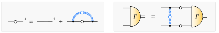
Figure 1: (Color online) Left panel: quark DSE (2) in rainbow truncation. Right panel: schematics of the meson BSE (3) and diquark BSE (5) in ladder truncation.

II.2 Quarks

The Dyson-Schwinger equation for the quark propagator in rainbow truncation is illustrated in the left panel of Fig. 1 and reads

$$S(p)^{-1}=Z_{2}\,(i\not{p}+m_{0})+\frac{4}{3}\int\limits_{q}\mathcal{G}(k^{2})\,\frac{T_{k}^{\mu\nu}}{k^{2}}\,\gamma^{\mu}\,S(q)\,\gamma^{\nu}\,,$$ (2)

where $S(p)$ is the renormalized dressed quark propagator, $p$ and $k=p-q$ are the quark and gluon momenta, and $\int_{q}=\int d^{4}q/(2\pi)^{4}$ represents a four-momentum integration. $T^{\mu\nu}_{k}/k^{2}$ with $T^{\mu\nu}_{k}=\delta^{\mu\nu}-k^{\mu}k^{\nu}/k^{2}$ is the free gluon propagator, $\gamma^{\nu}$ is the bare quark-gluon vertex, and $\mathcal{G}(k^{2})$ is the effective interaction defined above in Eq. (1). Dirac and flavor indices have been omitted for simplicity and the factor $\nicefrac{{4}}{{3}}$ comes from the color trace. The bare current-quark mass $m_{0}$ is the input of the equation. The solution of Eq. (2) requires a renormalization procedure, the details of which can be found together with the general structure of the quark DSE in e.g., Maris and Roberts (1997); Maris and Tandy (1999).

$S(p)$ is an important ingredient in all of the following. We note that its solution as an input for the various BSEs described below must be known in a parabola-shaped region of the complex $p^{2}$ plane, the size of which is proportional to the mass of the respective bound state that it helps to constitute. As a result, a sophisticated numerical approach is needed and we refer the reader to Krassnigg (2009b) for a description of our particular solution method.

II.3 Mesons

In our framework mesons with total $q\bar{q}$ momentum $P$ and relative $q\bar{q}$ momentum $p$ are studied via the meson BSE. Its structure in RL truncation is shown in the right panel of Fig. 1 and reads

$$\Gamma_{\text{M}}(p,P)=-\frac{4}{3}\int\limits_{q}\mathcal{G}(k^{2})\,\frac{T_{k}^{\mu\nu}}{k^{2}}\gamma^{\mu}\chi_{\text{M}}(q,P)\,\gamma^{\nu}\,,$$ (3)

where $\Gamma_{\text{M}}(k;P)$ is the Bethe-Salpeter amplitude and $\chi_{\text{M}}(q;P)=S(q_{+})\,\Gamma_{\text{M}}(q;P)\,S(q_{-})$ is referred to as the Bethe-Salpeter wave function. The quark and antiquark propagators depend on the (anti)quark momenta $q_{+}=q+\eta P$ and $q_{-}=q-(1-\eta)P$, where $\eta\in[0,1]$ is a momentum partitioning parameter usually set to $1/2$ for systems of equal-mass constituents (which we do as well). The quark-antiquark interaction kernel is given by a ladder dressed-gluon exchange, whose dependence on the gluon momentum is characterized by the same effective interaction, Eq. (1), as in the quark DSE Eq. (2). The combined set of truncated equations (2) and (3) thus already by construction satisfies the axial-vector Ward-Takahashi identity.

The general dependence of the meson amplitude on the various four-momenta can be written in terms of $N$ covariant structures $T_{i}$ reflecting the quark and antiquark spins, together with scalar components $F_{i}$, $i=1,\ldots,N$ as

$$\Gamma_{\text{M}}(q;P)=\sum^{N}_{i=1}T_{i}(P;q;\gamma)\,F_{i}(q^{2},q\cdot P,P^{2})\;,$$ (4)

where semicolons separate four-vector arguments, and $N=4$ for mesons with total spin $J=0$ and $N=8$ otherwise (see e.g., Krassnigg and Blank (2011)). A detailed account of the $T_{i}$ for pseudoscalar and vector mesons as needed in our calculation can be found in Ref. Krassnigg (2009a).

The components are scalar functions of their three scalar arguments: the total momentum squared $P^{2}$, the relative momentum squared $q^{2}$, and an angular variable $q\cdot P$. Note that for an on-shell amplitude $P^{2}=-M^{2}$ is fixed, while one artificially varies $P^{2}$ in the solution process of the homogeneous BSE (see e.g., Blank and Krassnigg (2011); Blank (2011), where also all necessary details on the numerical solution method can be found). In the corresponding inhomogeneous vertex BSE on the other hand, one would have $P$ and therefore also $P^{2}$ as a completely independent variable (see, e.g. Bhagwat et al. (2007); Blank and Krassnigg (2011, 2010)). Thus, the on-shell scalar components $F_{i}(q^{2},q\cdot P,P^{2})$ effectively depend on the two variables $q^{2}$ and $q\cdot P$. The latter can be parameterized by the variable $z\in[-1,1]$ related to the cosine defining the angle between $P$ and $q$. With such a reparameterization in mind, the components $F_{i}$ can be expanded further in Chebyshev polynomials, which leaves Chebyshev moments of the $F_{i}$ as sole functions of $q^{2}$ (for details and an illustration of Chebyshev moments, see Maris and Roberts (1997); Krassnigg and Roberts (2004)).

For our case very few Chebyshev moments are sufficient to produce converged results. However, in the context of the decay processes we note that, as a result of the kinematics in the triangle diagram as shown below, one needs to know the Bethe-Salpeter amplitudes in a certain region for the relative momentum squared $p^{2}$ in the complex plane. We achieve this by a continuation of the relevant Chebyshev polynomials into the complex $p^{2}$ plane via a Taylor-expansion technique up to 4th order which yields a converged result.

II.4 Diquarks

The relevance of diquark degrees of freedom in hadron physics has been reviewed in Anselmino et al. (1993), and diquarks are in many respects conceptually similar to mesons. In our setup, diquark correlations appear as structures in a quark-quark system whose properties can depend on the truncation or the effective interaction. In particular, in RL truncation diquarks appear as timelike poles in the quark-quark $T-$Matrix, which is an unphysical result since diquarks are not color singlets but elements of an antisymmetric color antitriplet. This has been identified as a truncation artifact, i.e., diquarks disappear from the physical spectrum beyond RL truncation Bender et al. (1996). Nevertheless, the significance of diquark correlations as binding structures within baryons has become apparent in various baryon form-factor studies, see e.g. Cloet et al. (2009); Nicmorus et al. (2010a); Eichmann et al. (2010b); Eichmann (2011). Moreover, the diquark concept has received support from investigations of diquark confinement in Coulomb-gauge QCD Alkofer et al. (2006).

In our particular case the diquark BSE in RL truncation reads

$$\Gamma_{\text{D}}(p,P)\,C=-\frac{2}{3}\int\limits_{q}\mathcal{G}(k^{2})\,\frac{T_{k}^{\mu\nu}}{k^{2}}\gamma^{\mu}\chi_{\text{D}}(q,P)\,C\,\gamma^{\nu}\,,$$ (5)

where $C$ is the charge-conjugation matrix, $\Gamma_{D}$ is the diquark amplitude, $\chi_{\text{D}}(q;P)\,C=S(q_{+})\,\Gamma_{\text{D}}(q;P)\,C\,S(q_{-})$, and for all practical purposes the only difference to the meson BSE Eq. (3) is the color factor.

In the description of baryons as quark-diquark bound states and also for the description of baryonic transitions as given below one needs to know not only the diquark amplitudes but also the diquark propagator. A defining equation for this propagator can be consistently derived from the two-quark Dyson equation and reads schematically Eichmann (2009)

$$D^{-1}=\text{tr}\int\hskip 1.0pt\overline{\Gamma}\hskip 1.0pt_{D}\,S\,\Gamma_{D}\,S^{T}-\text{tr}\int\!\!\!\int\hskip 1.0pt\overline{\Gamma}\hskip 1.0pt_{D}\,K^{-1}\,\Gamma_{D}\,,$$ (6)

which still contains on-shell amplitudes $\Gamma_{D}$ resulting from Eq. (5). To obtain the propagator $D$ for general $P^{2}$ appropriate ansätze for the off-shell amplitudes are chosen Eichmann (2009). $K$ is the same quark-quark interaction kernel that enters Eqs. (3–5), and a bar on an amplitude denotes charge conjugation: $\hskip 1.0pt\overline{\Gamma}\hskip 1.0pt(q,P)=C\,\Gamma(-q,-P)^{T}C^{T}$.

II.5 Baryons

In this work baryons are interpreted as bound states of a quark and a diquark, which reduces the three-quark problem to an effective two-body problem derived via omission of three-quark interactions and a pole ansatz in the quark-quark $T$-matrix, see e.g., Oettel et al. (1998, 2000a); Eichmann et al. (2008a); Eichmann (2009). The interaction in the resulting equation is an iterative quark exchange, where in every iteration step the spectator quark and one quark inside the diquark exchange roles. This quark-diquark BSE is illustrated in Fig. 2 and reads

$$\Gamma_{\text{B}}^{\alpha}(p,P)=c^{(\alpha\beta)}\!\!\int\limits_{k}K_{\text{Q-DQ}}^{\alpha\beta}\,S(k_{q})D^{\beta\beta^{\prime}}(k_{d})\,\Gamma_{\text{B}}^{\beta^{\prime}}(k,P)\,,$$ (7)

where $\Gamma_{\text{B}}^{\alpha}$ are the quark-diquark amplitudes of the respective baryon. Their general Dirac-Lorentz structure is described e.g. in Refs. Oettel et al. (1998); Eichmann (2009) and their decomposition in terms of covariant basis elements and Lorentz-invariant components is analogous to the previously discussed case of a meson amplitude, i.e., Eq. (4) and below. The quark-diquark exchange kernel is given by

$$K_{\text{Q-DQ}}^{\alpha\beta}=\Gamma_{\text{D}}^{\beta}(k_{r},k_{d})\,S^{T}(q)\,\hskip 1.0pt\overline{\Gamma}\hskip 1.0pt_{\text{D}}^{\alpha}(p_{r},p_{d})\,,$$ (8)

with $p_{q,d}$ and $k_{q,d}$ being the external and internal quark and diquark momenta and $p_{r}$, $k_{r}$ the relative momenta that enter the diquark amplitudes, cf. Fig. 2.

The treatment of light baryons such as the nucleon and $\Delta$ in the quark-diquark approach usually retains the lightest diquark degrees of freedom, i.e., scalar and axial-vector diquarks. The $\Delta$ baryon then involves only axial-vector diquark correlations whereas the nucleon contains both. As a consequence, the $\Delta N\pi$ coupling will involve axial-axial contributions as well as axial-scalar diquark transitions. The superscripts in Eqs. (7–8) account for both kinds of diquarks and an implicit sum over these indices is understood: $\Gamma^{\alpha}$ are scalar ($\alpha=0$) or axial-vector diquark amplitudes ($\alpha=1\dots 4$) obtained from their respective diquark BSEs (5), and $D^{00}$ and $D^{\beta\beta^{\prime}}$ denote the scalar and axial-vector diquark propagators, respectively. The color-flavor trace in Eq. (7) reads $c^{(00)}=-c^{(\alpha\beta)}=-\nicefrac{{1}}{{2}}$ and $c^{(0\alpha)}=c^{(\alpha 0)}=\nicefrac{{\sqrt{3}}}{{2}}$ for the nucleon, whereas in the case of the $\Delta$ it is given by $c^{(\alpha\beta)}=-1$. For details on the solution of the quark-diquark BSE we refer the reader to Refs. Oettel et al. (2002); Eichmann (2009).

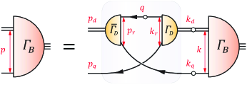
Figure 2: (Color online) The quark-diquark BSE, Eq. (7).

III Hadronic decays

Given a certain truncation of the DSE-BSE system, one can compute observables involving various currents through a consistent construction of the relevant invariant transition matrix elements. In our case we consider transitions between three hadrons and need a quark-level picture of the corresponding matrix elements. In the meson case, for RL truncation one arrives at a so-called triangle diagram Jarecke et al. (2003), depicted in Fig. 3, which corresponds to a generalized impulse approximation. Analogous diagrams are used at this level for, e.g., meson electromagnetic form factors Maris and Tandy (2000a). For baryons an appropriate construction is also possible and given below.

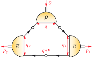
Figure 3: (Color online) The $\rho\pi\pi$ triangle diagram, Eq. (10).

III.1 Mesons: $\rho\to\pi\pi$

For the meson sector we investigate the $\rho\to\pi\pi$ transition which, in terms of Lorentz quantum numbers, corresponds to an $VPP$-vertex. As in the usual kinematical setup for a two-body decay one has the total $\rho-$meson momentum $Q$ and the relative momentum of the pion decay products $P=(P_{2}-P_{1})/2$. All mesons are on-shell, i.e. $Q^{2}=-m_{\rho}^{2}$ and $P_{1}^{2}=P_{2}^{2}=-m_{\pi}^{2}$, which entails $P\cdot Q=0$. Due to the transversality of the $\rho$-meson the most general Dirac-Lorentz structure of the transition can be parametrized as

$$\Lambda_{\rho\pi\pi}^{\mu}=2P^{\mu}\,g_{\rho\pi\pi}\,,$$ (9)

where $g_{\rho\pi\pi}$ is its dimensionless coupling constant. The corresponding triangle diagram is illustrated in Fig. 3 and reads

$$\Lambda_{\rho\pi\pi}^{\mu}=\text{tr}\int\limits_{q}\hskip 1.0pt\overline{\Gamma}\hskip 1.0pt_{\pi}(q_{2},P_{2})\,S(q+P)\,\hskip 1.0pt\overline{\Gamma}\hskip 1.0pt_{\pi}(q_{1},P_{1})\,\chi_{\rho}^{\mu}(q,Q),$$ (10)

where the $\hskip 1.0pt\overline{\Gamma}\hskip 1.0pt_{\pi}$ are the (charge-conjugated) on-shell pion amplitudes, i.e. the canonically normalized solutions of their homogeneous BSEs, $S$ is the renormalized dressed quark propagator obtained from its DSE, and $\chi_{\rho}^{\mu}$ is the $\rho-$meson wave function defined in connection with Eq. (3). The traces in color and flavor space yield a factor $3\sqrt{2}$ in front of the integral, cf. App. B.

More generally, the $\rho\pi\pi$ transition matrix element corresponds to the coupling of the pion to an external vector current. Specifically, if the $\rho-$meson amplitude that appears in Eq. (10) were replaced by the dressed quark-photon vertex, evaluated at arbitrary momentum squared $Q^{2}$, the respective triangle diagram would constitute the pion’s electromagnetic form factor: $\Lambda_{\gamma\pi\pi}^{\mu}=2P^{\mu}F_{\pi}(Q^{2})$. As the photon fluctuates into $\rho^{0}$, the dressed quark-photon vertex, obtained from its inhomogeneous BSE, self-consistently develops a $\rho-$meson pole whose on-shell residue is proportional to the $\rho-$meson amplitude $\Gamma^{\mu}_{\rho}$ Maris and Tandy (2000a). Such a purely transverse component is an important ingredient in various hadronic form-factor studies where it contributes typically $\sim 50\%$ to $\pi$, $N$ and $\Delta$ squared electromagnetic radii Maris and Tandy (2000a); Bhagwat and Maris (2008); Eichmann et al. (2008b, 2010b). Consequently, the residue of the pion form factor at the $\rho-$meson pole $Q^{2}=-m_{\rho}^{2}$ is proportional to $g_{\rho\pi\pi}$:

$$F_{\pi}(Q^{2}=-m_{\rho}^{2})\longrightarrow\frac{f_{\rho}\,m_{\rho}}{Q^{2}+m_{\rho}^{2}}\,\frac{g_{\rho\pi\pi}}{\sqrt{2}}\,.$$ (11)

In the present study we are primarily interested in the value of $g_{\rho\pi\pi}$ on the mass shell $Q^{2}=-m_{\rho}^{2}$. In a covariant formalism such as ours, one may simply choose a frame of reference—in our case the rest frame of the decaying particle—by setting $Q=(0,0,0,im_{\rho})$ and $P=(0,0,\kappa,0)$, where $\kappa^{2}=m_{\rho}^{2}/4-m_{\pi}^{2}$. Then, together with Eq. (10), $g_{\rho\pi\pi}$ is straightforward to evaluate numerically.

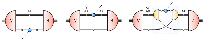
Figure 4: (Color online) Decomposition of the $\Delta N\pi$ transition matrix element in the quark-diquark model, Eqs. (16–17). Seagull terms are neglected. ’SC’ and ’AX’ denote the types of diquarks (i.e., scalar and axial-vector) that can appear in combination with the nucleon and $\Delta$ bound-state amplitudes.

III.2 Baryons: $\Delta\to N\pi$

In the baryon case, the coupling of an on-shell nucleon and $\Delta-$baryon to a pseudoscalar current is described by the pseudoscalar transition form factor $G_{\Delta N\pi}(Q^{2})$. The $\Delta$-baryon is a spin-3/2 particle and is thus represented by a Rarita-Schwinger spinor. Combined with the restriction to positive energies for the nucleon and $\Delta$, the most general Dirac-Lorentz structure of the respective interaction vertex is given by

$$\Lambda^{\mu}_{\text{\tiny{$\Delta N$}}\pi}=G_{\text{\tiny{$\Delta N$}}\pi}(Q^{2})\,\frac{Q^{\nu}}{2M_{N}}\,\Lambda^{+}_{N}(P_{f})\,\mathbb{P}^{\nu\mu}_{\Delta}(P_{i})\,,$$ (12)

where $P_{i}$, $P_{f}$ are the incoming $\Delta$ and outgoing nucleon momenta, $Q=P_{f}-P_{i}$ is the pion momentum, and $\Lambda^{+}_{B}(k)=(\mathbf{1}+\hat{\not{k}})/2$ is the positive-energy projector of the baryon with $\hat{k}$ being the respective normalized momentum $\hat{P}_{i}$ or $\hat{P}_{f}$. The Rarita-Schwinger projector of the $\Delta$ reads

$$\mathbb{P}^{\nu\mu}_{\Delta}(k)=\Lambda^{+}_{\Delta}(k)\left(T_{k}^{\nu\mu}-\frac{1}{3}\,\gamma_{T}^{\nu}\gamma_{T}^{\mu}\right),$$ (13)

where $T^{\nu\mu}_{k}$ is a transverse projector with respect to $k$ and the $\gamma-$matrices $\gamma^{\mu}_{T}$ are transverse to $k$ as well.

At the quark level, the coupling of nucleon and $\Delta$ to a pseudoscalar current is represented by the quark-pseudoscalar vertex $\Gamma_{5}$. The latter satisfies an inhomogeneous BSE which has the same structure as Eq. (3) except for an additional inhomogeneous term on the right-hand side Maris and Roberts (1997):

$$\Gamma_{5}(p,Q)=Z_{4}\,i\gamma_{5}-\frac{4}{3}\int\limits_{q}\mathcal{G}(k^{2})\,\frac{T_{k}^{\mu\nu}}{k^{2}}\gamma^{\mu}\chi_{5}(q,Q)\,\gamma^{\nu}\,.$$ (14)

Its residue at the pion pole $Q^{2}=-m_{\pi}^{2}$ is proportional to the homogeneous pion amplitude $\Gamma_{\pi}$ (cf. also Maris and Roberts (1997); Blank and Krassnigg (2010)):

$$\Gamma_{5}(p,Q)\longrightarrow\frac{Z_{4}}{Z_{2}}\,\frac{f_{\pi}m_{\pi}^{2}}{2m_{0}}\,\frac{1}{Q^{2}+m_{\pi}^{2}}\,\Gamma_{\pi}(p,Q)\,,$$ (15)

where $f_{\pi}$ is the (calculated) pion decay constant and $m_{0}$ is the bare current-quark mass that enters the quark DSE (2). The solution for $\Gamma_{5}$ provides an off-shell expression for the pion amplitude $\Gamma_{\pi}$ and thereby allows to compute the pseudoscalar transition form factor at spacelike momenta $Q^{2}>0$. Then, $G_{\Delta N\pi}(Q^{2})$ corresponds to the form factor obtained from $\Gamma_{\pi}(p,Q)$ in Eq. (15), where the pion pole as well as its residue are removed, and its on-shell value is the $\Delta N\pi$ coupling constant $G_{\Delta N\pi}(-m_{\pi}^{2})=g_{\Delta N\pi}$.

For the $\Delta\to N\pi$ system the construction analogous to Eq. (10) is more complex since there are diquarks as well as quarks present as constituents of the states involved in the transition. Moreover, the pion will not only interact with the quarks and diquarks directly but can couple to the quark-diquark kernel as well, i.e. impulse-approximation diagrams alone are no longer sufficient in studying the $\Delta\to N\pi$ transition.

A systematic procedure to derive the coupling of a baryon to an external current is the gauging-of-equations method of Refs. Haberzettl (1997); Kvinikhidze and Blankleider (1999a, b). In the context of baryon electromagnetic form factors it has been applied to the quark-diquark model Oettel et al. (2000b) as well as the three-quark approach Eichmann (2011). The starting point is to identify the current with the residue of the ’gauged’ quark-diquark (or three-quark) $T-$matrix on the baryon’s mass shell. Upon exploiting the relation between the $T-$matrix and the kernel of the respective bound-state equation, the hadronic matrix elements of the current are obtained as a sum of diagrams that describe the coupling of the current to all ingredients at the constituent level, i.e. in our case to the quark and diquark propagators as well as the quark-diquark kernel. The procedure can be applied for mesons as well where, in the case of a rainbow-ladder quark-antiquark kernel, the triangle diagram of Fig. 3 is recovered.

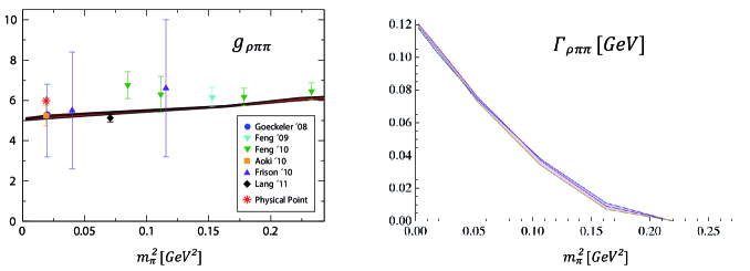
Figure 5: (Color online) Left panel: Evolution of the $\rho\pi\pi$ coupling with the pion mass squared. The experimental point is indicated by the star and the symbols denote lattice data from Refs. Gockeler et al. (2008); Feng et al. (2009, 2010); Aoki et al. (2010); Frison et al. (2010); Lang et al. (2011). For better readability the point of the Göckeler group is shifted slightly to the right. Right panel: The decay width of the $\rho$-meson versus the pion mass squared. The width of the bands illustrates the dependence on $\omega$ (see text).

The generalization of the method from an electromagnetic to a pseudoscalar current, as well as different kinds of baryons in the initial and final state, is straightforward. The resulting diagrams are displayed in Fig. 4 and involve impulse-approximation couplings to the quarks and diquarks as well as a coupling to the exchanged quark that appears in the quark-diquark kernel. In principle there would be further diagrams that contain seagulls, i.e., pseudoscalar couplings to the diquark amplitudes. For electromagnetic form factors such seagull contributions are typically small Cloet et al. (2009); Eichmann (2009) but necessary to ensure electromagnetic gauge invariance; however, in the present case we do not consider them further. The $\Delta N\pi$ transition matrix element is then decomposed as

$$\Lambda^{\mu}_{\text{\tiny{$\Delta N$}}\pi}=\Lambda_{\text{Q}}^{\mu}+\Lambda_{\text{DQ}}^{\mu}+\Lambda_{\text{EX}}^{\mu}\,,$$ (16)

where the three contributions are given by

$$\begin{split}\Lambda_{\text{Q}}^{\mu}&=\int\left[\hskip 1.0pt\overline{\Gamma}\hskip 1.0pt_{N}^{\alpha}\,\chi_{\pi}\,\Gamma_{\Delta}^{\beta\mu}\right]D^{\alpha\beta}\,,\\ \Lambda_{\text{DQ}}^{\mu}&=\int\left[\hskip 1.0pt\overline{\Gamma}\hskip 1.0pt_{N}^{\alpha}\,S\,\Gamma_{\Delta}^{\beta\mu}\right]D^{\alpha\alpha^{\prime}}\Gamma_{\text{D}\pi}^{\alpha^{\prime}\beta^{\prime}}D^{\beta^{\prime}\beta}\,,\\ \Lambda_{\text{EX}}^{\mu}&=\int\!\!\!\int\left[\hskip 1.0pt\overline{\Gamma}\hskip 1.0pt_{N}^{\alpha}\,S\,\Gamma_{\text{D}}^{\beta^{\prime}}\chi_{\pi}^{T}\,\hskip 1.0pt\overline{\Gamma}\hskip 1.0pt_{\text{D}}^{\alpha^{\prime}}\,S\,\Gamma_{\Delta}^{\beta\mu}\right]D^{\alpha\alpha^{\prime}}D^{\beta\beta^{\prime}}\,.\\ \end{split}$$ (17)

Here we suppressed the explicit momentum dependencies for brevity. The kinematics are analogous to the electromagnetic form-factor case and are described, e.g., in App. C.1 of Ref. Nicmorus et al. (2010a). $\Gamma_{N}^{\alpha}$ and $\Gamma_{\Delta}^{\beta\mu}$ are the quark-diquark amplitudes for the nucleon and $\Delta-$baryon; $\chi_{\pi}=S\,\Gamma_{\pi}S$ is the pion (off-shell) Bethe-Salpeter wave function obtained through the pseudoscalar vertex (15); $D^{\alpha\beta}$ is the diquark propagator; $\Gamma_{\text{D}}^{\alpha}$ is the diquark amplitude; and $\Gamma_{\text{D}\pi}^{\alpha\beta}$ is the vertex that describes the coupling of the pion to a diquark propagator. If an axial-vector diquark is involved, $\alpha,\beta=1\dots 4$ are Lorentz indices. Scalar-axialvector transitions, originating from the scalar-diquark component in the nucleon, can only occur in $\Lambda_{\text{DQ}}^{\mu}$ and $\Lambda_{\text{EX}}^{\mu}$; in that case: $\alpha=0$, and $D^{00}$ denotes the scalar diquark propagator and $\Gamma_{\text{D}\pi}^{0\beta}$ the scalar-axialvector transition vertex induced by the pion.

We note that all ingredients of Eq. (17) are determined self-consistently: Eqs. (2), (5–7) and (14) provide the dressed quark propagator, the scalar and axial-vector diquark amplitudes and propagators, the baryon amplitudes and the pseudoscalar vertex. The diquark-pion vertices are obtained in analogy to Eq. (10), i.e. through respective triangle diagrams. The color and flavor traces in Eq. (17) are worked out explicitly in App. B.

IV Results and Discussion

The building blocks of the $\rho\rightarrow\pi\pi$ and $\Delta\rightarrow N\pi$ transition matrix elements have been determined in the previous sections and we proceed with computing Eqs. (10) and (16) numerically. The Lorentz-invariant coupling constants $g_{\rho\pi\pi}$ and $g_{\text{\tiny{$\Delta N$}}\pi}$ are extracted via appropriate momentum contractions and Dirac traces, cf. Eq. (31). Since within our chosen truncations the ingredients of the equations for $g_{\rho\pi\pi}$ and $g_{\text{\tiny{$\Delta N$}}\pi}$ are computed selfconsistently, the effective quark-gluon coupling defined in Eq. (1) is the only model parametrization with impact upon the results. We explore the sensitivity to this ansatz by varying the $\omega$ parameter from its central value $\omega=0.4$ GeV which is indicated by the colored bands in the plots of this section.

IV.1 Mesons

Our result for $g_{\rho\pi\pi}$ at the physical $u/d$-quark mass is shown in Table 1 and compared to the experimental point given by the PDG Nakamura et al. (2010). In Fig. 5 we plot $g_{\rho\pi\pi}$ as a function of the pion mass squared and compare to recent lattice results Gockeler et al. (2008); Feng et al. (2009, 2010); Aoki et al. (2010); Frison et al. (2010); Lang et al. (2011).

The following observations are important: first, both the magnitude and $m_{\pi}^{2}$ dependence of our results are in agreement with lattice results, including a slight underestimation of the experimental value by about $15\%$. Second, the $\omega$ dependence of the result is small, which results from the ground-state characteristics of the $\pi$- and $\rho$-meson amplitudes regarding their dependence on the relative-momentum squared. This second point also solidifies the result of Jarecke et al. (2003) where only the central value of our band, $\omega=0.4$ GeV was used.

Next, the very weak dependence on $m_{\pi}^{2}$ compares well to analyses using chiral perturbation theory Hemmert et al. (1998); Hanhart et al. (2008); Pelaez et al. (2010), where one concludes from the strong phase-space dependence of the decay width that the coupling’s $m_{\pi}^{2}$-dependence should indeed be close to zero. Consequently, when plotting the $\rho\to\pi\pi$ decay width in our approach as a function of $m_{\pi}^{2}$, Fig. 5, the falloff can be almost completely attributed to the phase-space factor in Eq. (30) and the width vanishes when the decay channel closes.

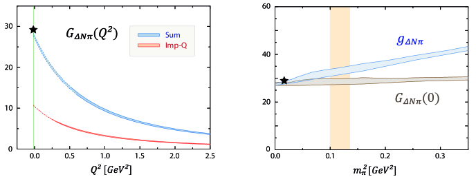
Figure 6: (Color online) Left panel: the transition form factor $G_{\Delta N\pi}$ as a function of the squared pion momentum $Q^{2}$. The upper band corresponds to the full result and the lower band shows the impulse-approximation value where the pion couples to the quark line only. The width of the bands again shows the dependence on $\omega$. The solid lines are the results of the calculation in the kinematically allowed regions whereas the dashed lines are the respective dipole fits, cf. Eq. (19). The pion mass shell $Q^{2}=-m_{\pi}^{2}$ is indicated by the vertical line and the star shows the experimental value $g_{\Delta N\pi}=G_{\Delta N\pi}(-m_{\pi}^{2})$. Right panel: Current-mass evolution of $g_{\Delta N\pi}$ (upper band) and $G_{\Delta N\pi}(Q^{2}=0)$ (lower band). The vertical shaded area depicts the $\omega$-dependent location of the threshold $M_{\Delta}=M_{N}+m_{\pi}$.

While comparison to experiment is favorable, the small difference between our result and the experimental value for $g_{\rho\pi\pi}$ warrants some discussion. The present model calculation uses a simple truncation, but an effective interaction which is fitted to the pion mass and underestimates the $\rho$-meson mass by about $5\%$. While the resulting kinematical mismatch is responsible for a small part of the difference, the main contributions are others. Even though one has to expect some effect from non-resonant corrections to RL truncation, the main improvement would be a self-consistent treatment of the $\rho$ meson as a resonance, i.e., an inclusion of an explicit $\pi\pi$ decay channel in the interaction kernel of the vector-meson BSE, in which, of course, also a different (refitted) effective interaction would have to be used. However, such an approach is much more involved than the present one and clearly beyond the scope of this study, in particular for the baryon case. In addition, the reasonably small difference to the experimental value of $g_{\rho\pi\pi}$ gives reason to expect that for this particular transition the present approach is at least a reliable gauge for future studies and results.

	$m_{\pi}$	$m_{\rho}$	$M_{N}$	$M_{\Delta}$	$g_{\rho\pi\pi}$	$g_{\text{\tiny{$\Delta N$}}\pi}$
This work	$0.14$	$0.74$	$0.94$	$1.28$	$5.20$	$28.1$
Experiment	$0.14$	$0.77$	$0.94$	$1.23$	$5.98$	$29.4$

Table 1: Comparison of our summarized mass and coupling values at the physical point for the central value of the $\omega$ band to corresponding experimental data. The pion mass is fitted to experiment, all other numbers are predictions of the model with no further parameters adjusted or introduced. The masses are given in GeV; the coupling constants are dimensionless.

IV.2 Baryons

The decay width of the $\Delta-$baryon is governed almost exclusively by the strong interaction, namely via the decay into the nucleon and a pion. The only other decay channel, the electromagnetic $\Delta\rightarrow N\gamma$ transition, has a branching fraction of less than $1\%$. Experimentally, $\Gamma_{\Delta}=118(2)$ MeV Nakamura et al. (2010), from which the corresponding coupling strength $g_{\text{\tiny{$\Delta N$}}\pi}=29.4(2)$ can be inferred via Eq. (30). Different conventions that are commonly employed in the literature read

$$\frac{g_{\text{\tiny{$\Delta N$}}\pi}}{2M_{N}}=\frac{g^{\prime}_{\text{\tiny{$\Delta N$}}\pi}}{m_{\pi}}=g^{\prime\prime}_{\text{\tiny{$\Delta N$}}\pi}\,,$$ (18)

with $g^{\prime}_{\text{\tiny{$\Delta N$}}\pi}\approx 2.16$ and $g^{\prime\prime}_{\text{\tiny{$\Delta N$}}\pi}\approx 15.7$ GeV^-1.

For general off-shell momenta the $\Delta\rightarrow N\pi$ coupling is described by the pseudoscalar transition form factor $G_{\text{\tiny{$\Delta N$}}\pi}(Q^{2})$ which we obtain from Eqs. (16) and (31). To compute the $Q^{2}-$dependence of the form factor we work in the Breit frame where the pion momentum is given by $Q=(0,0,|Q|,0)$. This has the advantage that the relative momenta in the baryon amplitudes are real and no continuation into the complex plane is necessary. However, due to the difference in the nucleon and $\Delta$ masses, the singularity structure in the quark and diquark propagators imposes kinematical constraints on the accessible $Q^{2}$ region from both below and above. Hence, to obtain the form factor $g_{\text{\tiny{$\Delta N$}}\pi}=G_{\text{\tiny{$\Delta N$}}\pi}(Q^{2}=-m_{\pi}^{2})$ at the pion mass, we fit our results at spacelike $Q^{2}$ with a dipole form:

$$G_{\text{Dipole}}(Q^{2})=\frac{G_{\text{\tiny{$\Delta N$}}\pi}(0)}{\left(1+Q^{2}/\Lambda_{\pi}^{2}\right)^{2}},$$ (19)

where $G_{\text{\tiny{$\Delta N$}}\pi}(0)$ and $\Lambda_{\pi}$ are free fit parameters.

Our result for the transition form factor $G_{\text{\tiny{$\Delta N$}}\pi}(Q^{2})$ at the physical $u/d$ mass is shown in the left panel of Fig. 6. Its computed value in the kinematically allowed range is plotted as a band with solid margins, where the width of the band corresponds to the model parameter $\omega$, whereas the fit results in the unaccessible region are shown as dashed lines. The resulting value of the strong coupling constant, $g_{\text{\tiny{$\Delta N$}}\pi}=28.1$, is remarkably close to the experimental number. We also note that the $Q^{2}-$evolution of $G_{\text{\tiny{$\Delta N$}}\pi}(Q^{2})$ is in good agreement with the lattice data of Ref. Alexandrou et al. (2010).

In general the dipole fits work very well and provide an adequate representation of the form factor $G_{\text{\tiny{$\Delta N$}}\pi}$ at spacelike values of the squared pion momentum. As described in connection with Eqs. (14–15), the $Q^{2}-$evolution of the form factor is governed by the pseudoscalar vertex $\Gamma_{5}$ which includes all pseudoscalar-meson poles, i.e. both the pion’s ground state as well as its excitations. While the pion ground-state pole and its residue were removed from Eq. (15) to obtain $G_{\text{\tiny{$\Delta N$}}\pi}$, the remaining excited states are still encoded in the vertex, hence the form factor $G_{\text{\tiny{$\Delta N$}}\pi}$ must diverge at the respective pole locations. Indeed we find that the dipole mass $\Lambda_{\pi}$ in Eq. (19) roughly coincides with the mass of the first excited state in the $0^{-+}$ channel which in RL trunctation, at the $u/d$ mass and for the central $\omega$ value, is obtained as $m_{\pi^{\star}}=1.1$ GeV Krassnigg and Maris (2005).

The left panel of Fig. 6 also includes the (quark-) impulse-approximation contribution to $G_{\text{\tiny{$\Delta N$}}\pi}$, i.e. the first diagram in Fig. 4 corresponding to $\Lambda_{\text{Q}}^{\mu}$ of Eq. (16). Here the diquark is merely a spectator and, since the $\Delta-$baryon only involves axial-vector diquark degrees of freedom, only an axial-vector diquark propagator can appear in that diagram. Fig. 6 shows that such a direct coupling to the quark provides roughly one third of the value of $G_{\text{\tiny{$\Delta N$}}\pi}$. The axial-axial contributions stemming from the second and third diagrams are comparatively small and contribute $\sim 10\%$ to the full result. The remainder owes in equal parts to the axial-scalar transitions that are generated from the transition vertex $\Gamma_{\text{D}\pi}^{0\beta}$ in the second diagram and the axial-scalar contribution $\Gamma_{\text{D}}^{\beta}\,\chi_{\pi}^{T}\,\hskip 1.0pt\overline{\Gamma}\hskip 1.0pt_{\text{D}}^{0}$ in the exchange diagram, cf. Eq. (17).

Once again, the current-quark mass dependence of the transition form factor can be studied by varying the current mass in the quark DSE. That change will be reflected in all ingredients that enter the transition matrix element. Similarly to the meson case, the overwhelming contribution to the mass dependence of the decay width $\Gamma_{\text{\tiny{$\Delta N$}}\pi}$ comes from the phase-space factor in Eq. (30). This is especially conspicuous in the form factor $G_{\text{\tiny{$\Delta N$}}\pi}(Q^{2}=0)$ at vanishing pion momentum, shown in the right panel of Fig. 6, which is practically independent of the current-quark mass. Similar features have been reported for $N$ and $\Delta$ electromagnetic form factors Nicmorus et al. (2010a); Eichmann (2011). The observation stays true for the $Q^{2}-$evolution, i.e. $G_{\text{\tiny{$\Delta N$}}\pi}(Q^{2})$ as well as its individual contributions retain their shape throughout the current-mass range if they are plotted over a dimensionless variable such as $Q^{2}/M_{N}^{2}$. Considering Eq. (19), this means that the dipole fit works also well for higher quark masses since the mass of the excited pion also varies with the current-quark mass in a similar fashion as $M_{N}$ and $M_{\Delta}$.

On the other hand, the value of $g_{\text{\tiny{$\Delta N$}}\pi}=G_{\text{\tiny{$\Delta N$}}\pi}(-m_{\pi}^{2})$ rises with the quark mass because of the current-mass dependent pion pole location. This property is also visible for $g_{\rho\pi\pi}$ in Fig. 5, albeit less pronounced, as the $\rho-$meson mass is non-zero in the chiral limit and therefore varies over a much smaller range when evolving the current-quark mass. The shaded area in Fig. 6 indicates the threshold position $M_{\Delta}=M_{N}+m_{\pi}$ where the decay channel closes, and the width of the band is again induced by the $\omega-$dependence which enters mainly through the mass of the $\Delta$, cf. Ref. Nicmorus et al. (2010b).

We finally note that in determining the $\Delta\to N\pi$ transition form factor we have neglected the pseudoscalar seagull terms which would appear in addition to the diagrams displayed in Fig. 6. Judging from the smallness of the electromagnetic seagulls in the case of electromagnetic form factors, this approximation might be well justified. The question of its validity can be settled by investigating the $\Delta\to N\pi$ transition in the three-quark framework of Ref. Eichmann (2011) where all such missing contributions, while no longer appearing explicitly, would be automatically included.

V Conclusions

We presented a calculation of the hadronic $\rho\to\pi\pi$ and $\Delta\rightarrow N\pi$ decays, as well as the pseudoscalar transition form factor $G_{\text{\tiny{$\Delta N$}}\pi}(Q^{2})$, in the framework of Dyson-Schwinger and covariant bound-state equations. A consistent construction for the decay diagrams was implemented. The $\rho\to\pi\pi$ transition was computed from the quark-antiquark Bethe-Salpeter equation in rainbow-ladder truncation whereas the $\Delta\to N\pi$ transition was studied within the covariant quark-diquark model. All ingredients are determined self-consistently which leaves a phenomenological ansatz for the quark-gluon coupling as the only model input.

The results in both cases compare well with experimental and lattice data. The $\rho\pi\pi$ coupling is underestimated by $\sim 15\%$ and slowly rises with the current-quark mass, in agreement with lattice results. A similar observation holds for the $\Delta\to N\pi$ coupling which agrees also well with the experimental result. We find that $G_{\text{\tiny{$\Delta N$}}\pi}(0)$ is practically independent of the current-quark mass. Consequently, the decay widths for $\rho$ and $\Delta$ are mainly governed by the available phase space.

The present calculation provides a first step towards a thorough investigation of hadron resonances and their decays within QCD. An important future direction in that respect would involve the implementation of explicit $\rho\pi\pi$ and $\Delta N\pi$ decay channels in the $\rho-$meson and $\Delta-$baryon bound-state equations. Such an extension would represent a considerable step beyond the rainbow-ladder truncation employed herein and contribute to a more realistic description of hadron resonances from their underlying dynamics in QCD.

Appendix A Matrix elements and decay widths

For the decay of a particle with momentum $p$ and mass $M$ into two decay products with momenta $p_{i}$ and masses $m_{i}$, with $p=\sum_{i}p_{i}$, the decay width is given by

$$\Gamma=\frac{I}{2M}\,|\mathcal{M}|^{2}\,,$$ (20)

where the squared transition matrix element $|\mathcal{M}|^{2}$ is averaged over the spins/polarizations, i.e.

$$\begin{split}|\mathcal{M}_{\rho\pi\pi}|^{2}&=\frac{1}{3}\sum_{\lambda}|\mathcal{M}_{\lambda}|^{2}\,,\\ |\mathcal{M}_{\Delta N\pi}|^{2}&=\frac{1}{4}\sum_{ss^{\prime}}|\mathcal{M}_{ss^{\prime}}|^{2}\end{split}$$ (21)

and a sum over all final states is implicit. The phase-space factor $I=\kappa/(4\pi M)$ involves the quantity

$$\kappa=\frac{\sqrt{\left(M^{2}-(m_{1}+m_{2})^{2}\right)\left(M^{2}-(m_{1}-m_{2})^{2}\right)}}{2M}$$ (22)

which in the rest frame of the decaying particle is given by $\kappa=|\bm{p_{1}}|=|\bm{p_{2}}|$; thus the decay width becomes

$$\Gamma=\frac{\kappa}{8\pi M^{2}}\,|\mathcal{M}|^{2}\,.$$ (23)

In the case $\rho\rightarrow\pi\pi$ one obtains specifically:

$$\mathcal{M}_{\lambda}=\Lambda^{\mu}_{\rho\pi\pi}\,\epsilon^{\mu}_{\lambda}\quad\Longrightarrow\quad|\mathcal{M}_{\rho\pi\pi}|^{2}=\frac{4}{3}\,\kappa_{\rho\pi\pi}^{2}\,g_{\rho\pi\pi}\,,$$ (24)

where from Eq. (22) and the kinematics in Fig. 3 one has

$$\kappa_{\rho\pi\pi}=\sqrt{m_{\rho}^{2}/4-m_{\pi}^{2}}=\sqrt{P^{2}}\,,$$ (25)

and the polarization vectors $\varepsilon_{\lambda}^{\mu}$ of the $\rho$-meson are normalized to $\varepsilon_{\lambda}^{\mu}\,\varepsilon_{\lambda^{\prime}}^{\mu}=\delta_{\lambda\lambda^{\prime}}$. In the case $\Delta\rightarrow N\pi$ Eq. (12) entails

$$\begin{split}\mathcal{M}_{ss^{\prime}}&=\hskip 1.0pt\overline{\mathrm{u}}\hskip 1.0pt_{s}\,\Lambda^{\mu}_{\text{\tiny{$\Delta N$}}\pi}\,\mathrm{u}^{\mu}_{s^{\prime}}=\frac{g_{\text{\tiny{$\Delta N$}}\pi}}{2M_{N}}\,\hskip 1.0pt\overline{\mathrm{u}}\hskip 1.0pt_{s}\,Q^{\mu}\,\mathrm{u}^{\mu}_{s^{\prime}}\,,\end{split}$$ (26)

where $Q$ is the pion momentum, and the nucleon and $\Delta$ spinors are normalized to

$$\sum_{s}\mathrm{u}_{s}\hskip 1.0pt\overline{\mathrm{u}}\hskip 1.0pt_{s}=2M_{N}\,\Lambda_{N}^{+}\,,\quad\sum_{s}\mathrm{u}_{s}^{\mu}\,\hskip 1.0pt\overline{\mathrm{u}}\hskip 1.0pt_{s}^{\nu}=2M_{\Delta}\,\mathbb{P}^{\mu\nu}_{\Delta}\,,$$ (27)

respectively. This yields

$$|\mathcal{M}_{\text{\tiny{$\Delta N$}}\pi}|^{2}=\frac{1}{6}\frac{M_{\Delta}}{M_{N}}\,\sigma\,\kappa_{\text{\tiny{$\Delta N$}}\pi}^{2}\,g_{\text{\tiny{$\Delta N$}}\pi}^{2}$$ (28)

with the spin sum

$$\sigma=\text{tr}\left\{\Lambda_{N}^{+}(P_{f})\,\Lambda_{\Delta}^{+}(P_{i})\right\}=1+\sqrt{1+\frac{\kappa_{\text{\tiny{$\Delta N$}}\pi}^{2}}{M_{\Delta}^{2}}}\,.$$ (29)

The strong decay widths in both cases are then given by

$$\Gamma_{\rho\pi\pi}=\frac{\kappa_{\rho\pi\pi}^{3}\,g_{\rho\pi\pi}^{2}}{6\pi m_{\rho}^{2}}\,,\quad\Gamma_{\text{\tiny{$\Delta N$}}\pi}=\frac{\sigma\,\kappa_{\text{\tiny{$\Delta N$}}\pi}^{3}\,g_{\text{\tiny{$\Delta N$}}\pi}^{2}}{48\pi M_{\Delta}M_{N}}\,.$$ (30)

To extract the coupling constants from the matrix elements in Eqs. (10) and (16), one has to perform appropriate momentum contractions and Dirac traces which yields:

$$\begin{split}g_{\rho\pi\pi}=\frac{P^{\mu}\Lambda_{\rho\pi\pi}^{\mu}}{2\kappa_{\rho\pi\pi}^{2}}\,,\quad g_{\text{\tiny{$\Delta N$}}\pi}=\frac{3M_{N}}{\sigma\kappa_{\text{\tiny{$\Delta N$}}\pi}^{2}}\,\text{tr}\left\{Q^{\mu}\Lambda^{\mu}_{\text{\tiny{$\Delta N$}}\pi}\right\}\,.\end{split}$$ (31)

Appendix B Color and flavor factors

While the color and flavor traces in the quark DSE (2) and meson and baryon bound-state equations, Eqs. (3, 5, 7), have already been worked out in the main text, we still have to perform these traces for the $\rho\rightarrow\pi\pi$ and $\Delta\rightarrow N\pi$ transition matrix elements (10) and (16).

We work in the $SU(2)_{f}$-isosymmetric limit and thus we have two degenerate quark flavors $u=\bigl{(}\begin{smallmatrix}1\\ 0\end{smallmatrix}\bigr{)}$ and $d=\bigl{(}\begin{smallmatrix}0\\ 1\end{smallmatrix}\bigr{)}$. They transform according to the fundamental representation of $SU(2)$, whereas the anti-quarks $\bar{u}=\bigl{(}\begin{smallmatrix}1\\ 0\end{smallmatrix}\bigr{)}$ and $\bar{d}=\bigl{(}\begin{smallmatrix}0\\ 1\end{smallmatrix}\bigr{)}$ transform according to the complex conjugated fundamental representation. These can be used to construct representation matrices of mesons as quark-antiquark, diquarks as quark-quark and baryons as quark-diquark bound states.

The $\pi$ and the $\rho$-mesons discussed in this article are isovector states with three isospin projections, which can be labeled by the corresponding electric meson charge. A possible representation is given by the matrices

$$\begin{split}&\mathsf{r_{+}}=|u\,\bar{d}\rangle=\frac{\sigma_{1}+i\sigma_{2}}{2}\,,\\ &\mathsf{r_{0}}\,=\frac{|u\,\bar{u}\rangle-|d\,\bar{d}\rangle}{\sqrt{2}}=\frac{\sigma_{3}}{\sqrt{2}}\,,\\ &\mathsf{r_{-}}=|d\,\bar{u}\rangle=\frac{\sigma_{1}-i\sigma_{2}}{2}\,,\end{split}$$ (32)

where the $\sigma_{i}$ are the Pauli matrices, and the flavor matrices are normalized to $\text{tr}\{\mathsf{r}_{i}^{\dagger}\,\mathsf{r}_{j}^{\dagger}\}=\delta_{ij}$. The color factors for the mesons are given by $\delta_{AB}$, where $A,B=1,2,3$ denote the quark indices.

The $\rho^{0}-$meson in the triangle diagram of Eq. (10) can couple to the upper and the lower quark line. The color trace in both diagrams equals $3$ whereas the Dirac traces yield an opposite sign: $(\Lambda^{\uparrow})_{\rho\pi\pi}^{\mu}=-(\Lambda^{\downarrow})_{\rho\pi\pi}^{\mu}$, where $\Lambda^{\uparrow}$ represents the expression in Eq. (10). The full color-flavor-Dirac trace of the $\rho^{0}\to\pi^{+}\pi^{-}$ transition then yields

$$-\text{tr}\{\mathsf{r}_{+}^{\dagger}\,\mathsf{r}_{-}^{\dagger}\,\mathsf{r}_{0}\}\,3\,\Lambda^{\uparrow}-\text{tr}\{\mathsf{r}_{+}^{\dagger}\,\mathsf{r}_{0}\,\mathsf{r}_{-}^{\dagger}\}\,3\,\Lambda^{\downarrow}=3\sqrt{2}\,\Lambda^{\uparrow}\,,$$

i.e. the color-flavor trace of Eq. (10) is $3\sqrt{2}$.

Similar to the mesonic case, for two degenerate flavors there exist four different diquarks, one of which is an isoscalar whereas the other three form an iso-triplet. The difference to mesons in flavor space is due to the different transformation properties of quarks and antiquarks. The representation for the diquark flavor matrices reads

$$\begin{split}\mathsf{s_{0}}&=\frac{|u\,d\rangle-|d\,u\rangle}{\sqrt{2}}=\frac{i\sigma_{2}}{\sqrt{2}}\,,\\ \mathsf{s_{1}}&=|u\,u\rangle=\frac{\mathbf{1}+\sigma_{3}}{2}\,,\\ \mathsf{s_{2}}&=\frac{|u\,d\rangle+|d\,u\rangle}{\sqrt{2}}=\frac{\sigma_{1}}{\sqrt{2}}\,,\\ \mathsf{s_{3}}&=|d\,d\rangle=\frac{\mathbf{1}-\sigma_{3}}{2}\,.\end{split}$$ (33)

The flavor factors for baryons in the quark-diquark picture are given by the Clebsch-Gordan coefficients according to the respective diquark content of the baryon. For proton and neutron they read

$$\begin{split}\mathsf{p}&=\left(\,u\;\Big{|}\,\sqrt{\tfrac{2}{3}}\,d\,,\,-\sqrt{\tfrac{1}{3}}\,u\,,\,0\,\right),\\ \mathsf{n}&=\left(\,d\;\Big{|}\,0\,,\,\sqrt{\tfrac{1}{3}}\,d\,,\,-\sqrt{\tfrac{2}{3}}\,u\,\right),\end{split}$$ (34)

where the first terms represent the isoscalar diquark contributions and the remaining three the contributions from the isovector channel in the same order as Eq. (33). The $\Delta$-baryons do not contain any contribution from the scalar diquark, and the corresponding Clebsch-Gordan construction yields

$$\begin{split}&\!\Delta^{++}=\Big{(}\,u\,,\,0\,,\,0\,\Big{)},\quad\Delta^{+}=\left(\,\sqrt{\tfrac{1}{3}}\,d\,,\,\sqrt{\tfrac{2}{3}}\,u\,,\,0\,\right),\\ &\!\Delta^{0}=\left(\,0\,,\,\sqrt{\tfrac{2}{3}}\,d\,,\,\sqrt{\tfrac{1}{3}}\,u\,\right),\quad\Delta^{-}=\Bigl{(}\,0,\,0,\,d\,\Bigr{)}.\end{split}$$ (35)

Finally, the color factors are $(\varepsilon_{ABC}/\sqrt{6})$ for the diquark amplitudes and $(\delta_{AC}/\sqrt{3})$ for the $N$ and $\Delta$ quark-diquark amplitudes, where $A,B$ are quark indices and $C$ is the diquark index.

In the case of the $\Delta^{++}\to p\pi^{+}$ transition the three contributions in Eq. (17) yield the following flavor traces:

$$\begin{split}\sum_{j}\mathsf{p}_{j}^{\dagger}\,\mathsf{r}_{+}^{\dagger}\,\Delta^{++}_{j}&\,,\quad\sum_{ij}\mathsf{p}_{i}^{\dagger}\,\Delta^{++}_{j}\,2\,\text{tr}\{\mathsf{s}_{i}^{\dagger}\,\mathsf{s}_{j}\,\mathsf{r}_{+}^{\dagger}\},\\ &\sum_{ij}\mathsf{p}_{i}^{\dagger}\,\mathsf{s}_{j}\,\mathsf{r}_{+}^{\dagger}\,\mathsf{s}_{i}^{\dagger}\,\Delta^{++}_{j}\,.\end{split}$$ (36)

Only the axial-vector diquark contributes to the $\Delta$ (hence $j=1,2,3$) whereas the nucleon has both scalar ($i=0$) and axial-vector diquark components ($i=1,2,3$). Combined with the color traces $+1$ for the impulse-approximation diagrams and $-1$ for the exchange diagrams the final result for the $\Delta^{++}\to p\pi^{+}$ transition matrix element in Eq. (16) reads

$$\Lambda=\textstyle{\sqrt{\frac{2}{3}}}\left[\Lambda_{\text{Q}}^{\text{AA}}-\Lambda_{\text{DQ}}^{\text{AA}}+\sqrt{3}\,\Lambda_{\text{DQ}}^{\text{SA}}+\textstyle{\frac{1}{2}}\,\Lambda_{\text{EX}}^{\text{AA}}-\textstyle{\frac{\sqrt{3}}{2}}\,\Lambda_{\text{EX}}^{\text{SA}}\right],$$

where the superscripts S and A refer to the scalar or axial-vector diquark content in the outgoing (left) and incoming (right) baryon amplitudes.

The remaining processes are obtained accordingly by replacing $\mathsf{p}$, $\Delta^{++}$ and $\mathsf{r_{+}}$ with the appropriate flavor structures of Eqs. (32) and (34–35). The bracket in the previous equation is identical in all cases whereas the prefactors become:

• $\pm\sqrt{\frac{2}{3}}$ for the transitions $\Delta^{++}\to p\pi^{+}$, $\Delta^{-}\to n\pi^{-}$;

• $-\frac{2}{3}$ for $\Delta^{+}\to p\pi^{0}$, $\Delta^{0}\to n\pi^{0}$;

• $\pm\frac{\sqrt{2}}{3}$ for $\Delta^{+}\to n\pi^{+}$ and $\Delta^{0}\to p\pi^{-}$.

For every initial state one has to sum over all final states via Eq. (20), hence one gets for both $\Delta^{+}$ and $\Delta^{0}$

$$\sqrt{\left\lvert\frac{2}{3}\right\rvert^{2}+\left\lvert\frac{\sqrt{2}}{3}\right\rvert^{2}}=\sqrt{\frac{2}{3}}\,,$$ (37)

and thus all flavor factors in the $\Delta N\pi$ system are the same.

References

- Faiman and Hendry (1969) D. Faiman and A. W. Hendry, Phys. Rev. 180, 1609 (1969).
- Feynman et al. (1971) R. P. Feynman, M. Kislinger, and F. Ravndal, Phys. Rev. D 3, 2706 (1971).
- Kim and Noz (1975) Y. S. Kim and M. E. Noz, Phys. Rev. D 12, 129 (1975).
- Koniuk and Isgur (1980) R. Koniuk and N. Isgur, Phys. Rev. D 21, 1868 (1980).
- Godfrey and Isgur (1985) S. Godfrey and N. Isgur, Phys. Rev. D 32, 189 (1985).
- Plessas et al. (1999) W. Plessas, A. Krassnigg, L. Theussl, R. F. Wagenbrunn, and K. Varga, Few-Body Syst. Suppl. 11, 29 (1999).
- Melde et al. (2007) T. Melde, W. Plessas, and B. Sengl, Phys. Rev. C 76, 025204 (2007).
- Kokoski and Isgur (1987) R. Kokoski and N. Isgur, Phys. Rev. D 35, 907 (1987).
- Close and Page (1995) F. E. Close and P. R. Page, Nucl. Phys. B 443, 233 (1995).
- Stassart and Stancu (1995) P. Stassart and F. Stancu, Z. Phys. A 351, 77 (1995).
- Le Yaouanc et al. (1975) A. Le Yaouanc, L. Oliver, O. Pene, and J. C. Raynal, Phys. Rev. D 11, 1272 (1975).
- Capstick and Roberts (1998) S. Capstick and W. Roberts, Phys. Rev. D 58, 074011 (1998).
- Theussl et al. (2001) L. Theussl, R. F. Wagenbrunn, B. Desplanques, and W. Plessas, Eur. Phys. J. A 12, 91 (2001).
- Krassnigg et al. (2003a) A. Krassnigg, W. Schweiger, and W. H. Klink, Few-Body Syst. Suppl. 14, 419 (2003a).
- Krassnigg et al. (2003b) A. Krassnigg, W. Schweiger, and W. H. Klink, Phys. Rev. C 67, 064003 (2003b).
- Biernat et al. (2010) E. P. Biernat, W. H. Klink, and W. Schweiger, 1008.0244 [nucl-th] .
- Kleinhappel and Schweiger (2010) R. Kleinhappel and W. Schweiger, 1010.3919 [nucl-th] .
- Singh and Mitra (1988) N. N. Singh and A. N. Mitra, Phys. Rev. D 38, 1454 (1988).
- Metsch et al. (2003) B. Metsch, U. Loring, D. Merten, and H. Petry, Eur. Phys. J. A 18, 189 (2003).
- Ricken et al. (2003) R. Ricken, M. Koll, D. Merten, and B. C. Metsch, Eur. Phys. J. A 18, 667 (2003).
- Guo et al. (2008) X.-H. Guo, K.-W. Wei, and X.-H. Wu, Phys. Rev. D 77, 036003 (2008).
- Oset et al. (2010) E. Oset et al., 1008.0466 [hep-ph] .
- Gockeler et al. (2008) M. Gockeler et al. (QCDSF), PoS LATTICE2008, 136 (2008).
- Feng et al. (2009) X. Feng, K. Jansen, and D. B. Renner, PoS LAT2009, 109 (2009).
- Feng et al. (2010) X. Feng, K. Jansen, and D. B. Renner, 1011.5288 [hep-lat] .
- Aoki et al. (2010) P.-. S. Aoki et al. (CS), PoS LATTICE2010, 108 (2010).
- Frison et al. (2010) J. Frison et al. (Budapest-Marseille-Wuppertal), 1011.3413 [hep-lat] .
- Lang et al. (2011) C. B. Lang, D. Mohler, S. Prelovsek, and M. Vidmar, 1105.5636 [hep-lat] .
- Alexandrou et al. (2010) C. Alexandrou, G. Koutsou, J. W. Negele, Y. Proestos, and A. Tsapalis, 1011.3233 [hep-lat] .
- Pichowsky and Lee (1997) M. A. Pichowsky and T. S. H. Lee, Phys. Rev. D 56, 1644 (1997).
- Pichowsky et al. (1999) M. A. Pichowsky, S. Walawalkar, and S. Capstick, Phys. Rev. D 60, 054030 (1999).
- Jarecke et al. (2003) D. Jarecke, P. Maris, and P. C. Tandy, Phys. Rev. C 67, 035202 (2003).
- Cattapan and Ferreira (2002) G. Cattapan and L. S. Ferreira, Phys. Rept. 362, 303 (2002).
- Pascalutsa et al. (2007) V. Pascalutsa, M. Vanderhaeghen, and S. N. Yang, Phys. Rept. 437, 125 (2007).
- Niskanen (1981) J. A. Niskanen, Phys. Lett. B 107, 344 (1981).
- Melde et al. (2009) T. Melde, L. Canton, and W. Plessas, Physical Review Letters 102, 132002 (2009).
- Sato and Lee (1996) T. Sato and T. S. H. Lee, Phys. Rev. C 54, 2660 (1996).
- Polinder and Rijken (2005) H. Polinder and T. A. Rijken, Phys. Rev. C 72, 065211 (2005).
- Wang (2008) Z.-G. Wang, Eur. Phys. J. C 57, 711 (2008).
- Aliev et al. (2010) T. M. Aliev, K. Azizi, and M. Savci, Nucl. Phys. A 847, 101 (2010).
- Alexandrou et al. (2009) C. Alexandrou et al., Phys. Rev. D 79, 014507 (2009).
- Maris (2007) P. Maris, AIP Conf. Proc. 892, 65 (2007).
- Krassnigg (2009a) A. Krassnigg, Phys. Rev. D 80, 114010 (2009a).
- Krassnigg and Blank (2011) A. Krassnigg and M. Blank, Phys. Rev. D 83, 096006 (2011).
- Maris and Tandy (2000a) P. Maris and P. C. Tandy, Phys. Rev. C 61, 045202 (2000a).
- Maris and Tandy (2000b) P. Maris and P. C. Tandy, Phys. Rev. C 62, 055204 (2000b).
- Holl et al. (2005) A. Holl, A. Krassnigg, P. Maris, C. D. Roberts, and S. V. Wright, Phys. Rev. C 71, 065204 (2005).
- Bhagwat and Maris (2008) M. S. Bhagwat and P. Maris, Phys. Rev. C 77, 025203 (2008).
- Anselmino et al. (1993) M. Anselmino, E. Predazzi, S. Ekelin, S. Fredriksson, and D. B. Lichtenberg, Rev. Mod. Phys. 65, 1199 (1993).
- Maris (2002) P. Maris, Few-Body Syst. 32, 41 (2002).
- Maris (2004) P. Maris, Few-Body Syst. 35, 117 (2004).
- Oettel et al. (1998) M. Oettel, G. Hellstern, R. Alkofer, and H. Reinhardt, Phys. Rev. C 58, 2459 (1998).
- Oettel et al. (2000a) M. Oettel, R. Alkofer, and L. von Smekal, Eur. Phys. J. A 8, 553 (2000a).
- Eichmann et al. (2008a) G. Eichmann, A. Krassnigg, M. Schwinzerl, and R. Alkofer, Annals Phys. 323, 2505 (2008a).
- Eichmann et al. (2009) G. Eichmann, I. C. Cloet, R. Alkofer, A. Krassnigg, and C. D. Roberts, Phys. Rev. C 79, 012202(R) (2009).
- Cloet et al. (2009) I. C. Cloet, G. Eichmann, B. El-Bennich, T. Klahn, and C. D. Roberts, Few Body Syst. 46, 1 (2009).
- Nicmorus et al. (2009) D. Nicmorus, G. Eichmann, A. Krassnigg, and R. Alkofer, Phys. Rev. D 80, 054028 (2009).
- Nicmorus et al. (2010a) D. Nicmorus, G. Eichmann, and R. Alkofer, 1008.3184 [hep-ph] .
- Eichmann (2009) G. Eichmann, Hadron properties from QCD bound-state equations, Ph.D. thesis, University of Graz (2009), 0909.0703 [hep-ph] .
- Eichmann et al. (2010a) G. Eichmann, R. Alkofer, A. Krassnigg, and D. Nicmorus, Phys. Rev. Lett. 104, 201601 (2010a).
- Sanchis-Alepuz et al. (2010) H. Sanchis-Alepuz, R. Alkofer, G. Eichmann, and S. Villalba-Chavez, PoS LC2010, 018 (2010).
- Eichmann (2011) G. Eichmann, 1104.4505 [hep-ph] .
- Alkofer et al. (2008) R. Alkofer, C. S. Fischer, and R. Williams, Eur. Phys. J. A 38, 53 (2008).
- Williams and Fischer (2009) R. Williams and C. S. Fischer, 0912.3711 [hep-ph] .
- Chang and Roberts (2010) L. Chang and C. D. Roberts, 1003.5006 [nucl-th] .
- Maskawa and Nakajima (1975) T. Maskawa and H. Nakajima, Prog. Theor. Phys. 54, 860 (1975).
- Aoki et al. (1991) K.-I. Aoki, T. Kugo, and M. G. Mitchard, Phys. Lett. B 266, 467 (1991).
- Kugo and Mitchard (1992) T. Kugo and M. G. Mitchard, Phys. Lett. B 286, 355 (1992).
- Bando et al. (1994) M. Bando, M. Harada, and T. Kugo, Prog. Theor. Phys. 91, 927 (1994).
- Munczek (1995) H. J. Munczek, Phys. Rev. D 52, 4736 (1995).
- Maris et al. (1998) P. Maris, C. D. Roberts, and P. C. Tandy, Phys. Lett. B 420, 267 (1998).
- Maris and Roberts (1997) P. Maris and C. D. Roberts, Phys. Rev. C 56, 3369 (1997).
- Holl et al. (2004) A. Holl, A. Krassnigg, and C. D. Roberts, Phys. Rev. C 70, 042203(R) (2004).
- Maris and Tandy (1999) P. Maris and P. C. Tandy, Phys. Rev. C 60, 055214 (1999).
- Fischer et al. (2008) C. S. Fischer, A. Maas, and J. M. Pawlowski, Annals Phys. 324, 2408 (2008).
- Binosi and Papavassiliou (2009) D. Binosi and J. Papavassiliou, Phys. Rept. 479, 1 (2009).
- Blank et al. (2011) M. Blank, A. Krassnigg, and A. Maas, Phys. Rev. D 83, 034020 (2011).
- Krassnigg (2009b) A. Krassnigg, PoS Confinement8, 75 (2009b).
- Blank and Krassnigg (2011) M. Blank and A. Krassnigg, Comput. Phys. Commun. 182, 1391 (2011).
- Blank (2011) M. Blank, Properties of quarks and mesons in the Dyson-Schwinger/Bethe-Salpeter approach, Ph.D. thesis, University of Graz (2011).
- Bhagwat et al. (2007) M. S. Bhagwat, A. Hoell, A. Krassnigg, C. D. Roberts, and S. V. Wright, Few-Body Syst. 40, 209 (2007).
- Blank and Krassnigg (2010) M. Blank and A. Krassnigg, To appear in the proceedings of “Quark Confinement and the Hadron Spectrum IX”, 1011.5772 [hep-ph] .
- Krassnigg and Roberts (2004) A. Krassnigg and C. D. Roberts, Nucl. Phys. A 737, 7 (2004).
- Bender et al. (1996) A. Bender, C. D. Roberts, and L. Von Smekal, Phys. Lett. B 380, 7 (1996).
- Eichmann et al. (2010b) G. Eichmann, R. Alkofer, C. S. Fischer, A. Krassnigg, and D. Nicmorus, 1010.0206 [hep-ph] .
- Alkofer et al. (2006) R. Alkofer, M. Kloker, A. Krassnigg, and R. F. Wagenbrunn, Phys. Rev. Lett. 96, 022001 (2006).
- Oettel et al. (2002) M. Oettel, L. Von Smekal, and R. Alkofer, Comput. Phys. Commun. 144, 63 (2002).
- Eichmann et al. (2008b) G. Eichmann, R. Alkofer, I. C. Cloet, A. Krassnigg, and C. D. Roberts, Phys. Rev. C 77, 042202(R) (2008b).
- Haberzettl (1997) H. Haberzettl, Phys. Rev. C 56, 2041 (1997).
- Kvinikhidze and Blankleider (1999a) A. N. Kvinikhidze and B. Blankleider, Phys. Rev. C 60, 044003 (1999a).
- Kvinikhidze and Blankleider (1999b) A. N. Kvinikhidze and B. Blankleider, Phys. Rev. C 60, 044004 (1999b).
- Oettel et al. (2000b) M. Oettel, M. Pichowsky, and L. von Smekal, Eur. Phys. J. A 8, 251 (2000b).
- Nakamura et al. (2010) K. Nakamura et al. (Particle Data Group), J. Phys. G 37, 075021 (2010).
- Hemmert et al. (1998) T. R. Hemmert, B. R. Holstein, and J. Kambor, J. Phys. G 24, 1831 (1998).
- Hanhart et al. (2008) C. Hanhart, J. R. Pelaez, and G. Rios, Phys. Rev. Lett. 100, 152001 (2008).
- Pelaez et al. (2010) J. R. Pelaez, C. Hanhart, J. Nebreda, and G. Rios, AIP Conf. Proc. 1257, 141 (2010).
- Krassnigg and Maris (2005) A. Krassnigg and P. Maris, J. Phys. Conf. Ser. 9, 153 (2005).
- Nicmorus et al. (2010b) D. Nicmorus, G. Eichmann, A. Krassnigg, and R. Alkofer, 1008.4149 [hep-ph] .