Effect of spin diffusion on current generated by spin motive force

Abstract

Spin motive force is a spin-dependent force on conduction electrons induced by magnetization dynamics. In order to examine its effects on magnetization dynamics, it is indispensable to take into account spin accumulation, spin diffusion, and spin-flip scattering since the spin motive force is in general nonuniform. We examine the effects of all these on the way the spin motive force generates the charge and spin currents in conventional situations, where the conduction electron spin relaxation dynamics is much faster than the magnetization dynamics. When the spin-dependent electric field is spatially localized, which is common in experimental situations, we find that the conservative part of the spin motive force is unable to generate the charge current due to the cancelation effect by the diffusion current. We also find that the spin current is a nonlocal function of the spin motive force and can be effectively expressed in terms of nonlocal Gilbert damping tensor. It turns out that any spin independent potential such as Coulomb potential does not affect our principal results. At the last part of this paper, we apply our theory to current-induced domain wall motion.

I Introduction

In a ferromagnetic system, dynamics of space-time dependent magnetization vector $\mathbf{M}(\mathbf{x},t)$ is described by the following phenomenological equation Zhang04PRL ; Thiaville05EPL ; Tatara06JPS ; Stiles07PRB

$$\frac{\partial\mathbf{M}}{\partial t} = -\gamma\mathbf{M}\times\mathbf{H}_{eff}+\frac{\alpha}{M_{s}}\mathbf{M}\times\frac{\partial\mathbf{M}}{\partial t}$$ (1)

$$+\frac{\mu_{B}}{eM_{s}}(\mathbf{j}_{s}\cdot\nabla)\mathbf{M}-\frac{\beta\mu_{B}}{eM_{s}^{2}}\mathbf{M}\times(\mathbf{j}_{s}\cdot\nabla)\mathbf{M}.$$

This is the Landau-Lifshitz-Gilbert (LLG) equation generalized to include the spin-transfer torque terms (last two terms). Here, $\mathbf{H}_{eff}$ is the functional derivative of energy with respect to $\mathbf{M}$, $\alpha$ is Gilbert damping constant, $M_{s}$ is saturation magnetization, $\mu_{B}$ is Bohr magneton, $e$ is electron charge, $\beta$ is nonadiabaticity, and $\mathbf{j}_{s}$ is spin polarized electric current given by difference between current by spin-up and spin-down electrons. LLG equation describes the dynamics of magnetization under applied electromagnetic fields. On the other hand, there exists a reciprocal process; temporal and spatial variation of magnetization induces additional electromagnetic fields on conduction electrons. These fields are spin-dependent and in general nonconservative. Thus the resulting spin-dependent motive force is called spin motive force (SMF). SMF is firstly predicted by Berger Berger86PRB and recently formulated by generalizing Faraday’s law Barnes07PRL . It is also suggested Zhang09PRL that SMF is also described by spin pumping effect Tserkovnyak02PRL . Recently, SMF and its effect is intensively studied Shibata09PRL ; Zhang10PRB ; Kim11Preprint ; Zhang09PRL ; Duine09PRB ; Ohe09APL ; Ohe09JAP ; Tserkovnyak08PRB ; Tserkovnyak09PRB ; Wong10PRB ; Hai09Nature ; Yang09PRL ; Saslow07PRB in this field.

Without any other perturbation, the explicit expressions of the induced spin electromagnetic fields are known as Shibata09PRL ; Tserkovnyak09PRB ; Tserkovnyak08PRB ; Zhang09PRL ; Zhang10PRB ; Volovik87JPC ; Kim11Preprint

$$E_{i}^{{\uparrow\downarrow}} = \pm\frac{\hbar}{2eM_{s}^{3}}\left(\partial_{t}\mathbf{M}\times\partial_{i}\mathbf{M}\right)\cdot\mathbf{M},$$ (2)

$$B_{i}^{{\uparrow\downarrow}} = \mp\frac{\hbar}{2eM_{s}^{3}}\epsilon_{ijk}(\partial_{j}\mathbf{M}\times\partial_{k}\mathbf{M})\cdot\mathbf{M},$$ (3)

where $\uparrow$ and $\downarrow$ stand for spin-up and down electrons. The fields generate spin-dependent Lorentz force $F_{s}^{{\uparrow\downarrow}}=e(\mathbf{E}_{i}^{{\uparrow\downarrow}}+\mathbf{v}^{{\uparrow\downarrow}}\times\mathbf{B}_{s}^{{\uparrow\downarrow}})$. While the term “motive force” refers to quantities of voltage dimension, the term SMF is sometimes used to denote $F_{s}^{\uparrow\downarrow}$. In this paper, we adopt the latter terminology. It is easily noticed that SMF is spin dependent, nonconservative, spatially varying, and localized in general situations. As one can see from Eqs. (2) and (3), SMF is usually too small to be measured directly. Another way is to study the effect of SMF on magnetization dynamics. Since SMF induces additional spin current, additional spin-transfer torque arises and it changes LLG equation. Consequently, LLG equation (without applied spin current) is modified as Zhang09PRL

$$\frac{\partial\mathbf{M}}{\partial t}=-\gamma\mathbf{M}\times\mathbf{H}_{eff}+\frac{1}{M_{s}}\mathbf{M}\times\left(\mathcal{D}\cdot\frac{\partial\mathbf{M}}{\partial t}\right),$$ (4)

where $\mathcal{D}$ is modified damping tensor given by

$$\mathcal{D}_{ij}=\alpha\delta_{ij}+\frac{\eta}{M_{s}^{4}}\sum_{k}(\mathbf{M}\times\partial_{k}\mathbf{M})_{i}(\mathbf{M}\times\partial_{k}\mathbf{M})_{j},$$ (5)

and $\eta=\mu_{B}\hbar\sigma/2e^{2}M_{s}$. Here, $\sigma$ is electrical conductivity.

However, the previous work has a crucial limitation that spin density has been considered to be constant while spin density in reality is nonuniform since SMF is spatially varying. The main consequence of the nonuniform spin density $n^{\uparrow\downarrow}(\mathbf{x},t)$ is diffusion current proportional to $-\nabla n^{\uparrow\downarrow}$, which suppresses the effect of SMF. Therefore, a realistic model should take into account spin accumulation (nonuniform spin density), diffusion and spin-flip scattering. The purpose of this paper is to find the spin density $n^{\uparrow\downarrow}$, diffusion current, total current induced by SMF, and their effect on magnetization dynamics in the presence of spin accumulation, diffusion, and spin-flip scattering. As one shall see in Sec. III, the solution of $n^{\uparrow\downarrow}$ in the most general situation is too complicated to study the effect on magnetization dynamics. To obtain simple analytic expressions, we take an approximation that spin-flip time is much shorter than the time scale of magnetization dynamics. As a final comment, our result does not assume any specific form of SMF. Thus, it remains valid for the modified SMF due to, for instance, nonadiabaticity Tserkovnyak08PRB , spin-orbit coupling Kim11Preprint , and other kinds of spin dependent electric field Sherman06arXiv .

Several previous works are closely related to our work. Spin drift-diffusion equation, which has similar form to our theory is suggested in Ref. Tserkovnyak08PRB . And, the effect on spin and charge current is investigated from Boltzmann equation in Ref. Zhang10PRB . We set our starting point as the equation of motion of conduction electrons in Ref. Zhang04PRL to make our analysis consistent with previous theories in this field. Different from the previous theories focusing on 1D, we successfully generalized our result to 3D, and found that nonconservative part of SMF plays a crucial role in current in a higher dimensional system. In Sec. III, we compare our result with the previous theory qualitatively and quantitatively. In addition, we investigated the effect of charge neutrality on our results. It turns out that charge neutrality potential does not change our principal results, charge current and spin current, even though it changes charge density and spin density. Furthermore, we show that any spin independent potential cannot alter our principal results, either.

This paper is organized as follows. In Sec. II, we construct the spin drift-diffusion equation and introduce variables. Then, we solve the equation in Sec. III, and discuss various implications. In Sec. IV, we apply our result to current-induced domain wall (DW) motion and briefly discuss the effect of spin diffusion. In Sec. V, we generalize our theory for general boundary condition and for general spin indendendent potentials. Finally, in Sec. VI, there are concluding remarks. Technical details are in Appendices.

II Model

II.1 Spin drift-diffusion equation

To construct the equation of $n^{\uparrow\downarrow}(\mathbf{x},t)$, we take the starting point as the equation of spin density $\mathbf{m}$ of conduction electrons Zhang04PRL ,

$$\frac{\partial\mathbf{m}}{\partial t}+\nabla\cdot J=-\frac{1}{\tau_{ex}M_{s}}\mathbf{m}\times\mathbf{M}-\langle\mathbf{\Gamma}\rangle.$$ (6)

Here, $J$ is spin current tensor, $\tau_{ex}=\hbar/SJ_{ex}$, and $S$ denotes the magnitude of spin of local magnetization. The left-hand side is based on the continuity equation. The first term on the right-hand side is the precession term due to the exchange coupling between conduction electrons and magnetization. $\langle\mathbf{\Gamma}\rangle$ includes the effect of spin scattering processes. Here, the second rank tensor $J$ is defined by

$$J=-\frac{\mu_{B}}{e}\mathbf{j}_{s}\otimes\frac{\mathbf{m}}{|\mathbf{m}|}.$$ (7)

The effect of the perpendicular component to $\mathbf{M}$ of Eq. (6) is already investigated by Zhang and Li Zhang04PRL , and they found the nonadiabatic term of LLG equation. In the absence of spin accumulation, the magnitude of $\mathbf{m}$ is constant, so it suffices to solve only the perpendicular component of the equation. However, in the presence of the spin accumulation, the magnitude variation of $\mathbf{m}$ should be also studied. We define spin number density $n_{s}\equiv|\mathbf{m}|/\mu_{B}$. Taking care of the fact that $n_{s}$ has space-time dependence, the parallel component of Eq. (6) to $\hat{m}\equiv\mathbf{m}/|\mathbf{m}|$ results in

$$\frac{\partial n_{s}}{\partial t}+\frac{1}{\mu_{B}}\hat{m}\cdot\langle\mathbf{\Gamma}\rangle=\frac{1}{e}\nabla\cdot\mathbf{j}_{s}.$$ (8)

It is convenient to separate the variables to that of up and down electrons. $n_{s}=n^{\uparrow}-n^{\downarrow}$ and $\mathbf{j}_{s}=\mathbf{j}^{\uparrow}-\mathbf{j}^{\downarrow}$. Here, $n^{\uparrow\downarrow}$ and $\mathbf{j}^{\uparrow\downarrow}$ denote spin number density of spin-up/down electrons and charge current density generated by spin-up/down electrons, respectively. Equation (8) is nothing but the continuity equation containing spin nonconserving processes described by $\mathbf{\Gamma}$. To obtain independent equations of spin-up/down electrons, we use the following continuity equation of total electron number density

$$\frac{\partial n_{e}}{\partial t}=\frac{1}{e}\nabla\cdot\mathbf{j}_{e},$$ (9)

where $n_{e}=n^{\uparrow}+n^{\downarrow}$ is electron number density and $\mathbf{j}_{e}=\mathbf{j}^{\uparrow}+\mathbf{j}^{\downarrow}$ is charge current density. Combining Eqs. (8) and (9), one obtains

$$\frac{\partial n^{\uparrow\downarrow}}{\partial t}\pm\frac{1}{2\mu_{B}}\hat{m}\cdot\langle\mathbf{\Gamma}\rangle=\frac{1}{e}\nabla\cdot\mathbf{j}^{\uparrow\downarrow}.$$ (10)

Note that $\mathbf{\Gamma}$ represents spin-flip scattering processes. As a simple model, we take the well-known form of spin-flip scattering,

$$\frac{1}{2\mu_{B}}\hat{m}\cdot\langle\mathbf{\Gamma}\rangle=\frac{n^{\uparrow}}{\tau^{\uparrow}}-\frac{n^{\downarrow}}{\tau^{\downarrow}},$$ (11)

where $\tau^{\uparrow}$ is characteristic time of the spin-flip scattering process from spin-up to -down state, and $\tau^{\downarrow}$ is similarly defined. Then,

$$\frac{\partial n^{\uparrow\downarrow}}{\partial t}+\frac{n^{\uparrow\downarrow}}{\tau^{\uparrow\downarrow}}-\frac{n^{\downarrow\uparrow}}{\tau^{\downarrow\uparrow}}=\frac{1}{e}\nabla\cdot\mathbf{j}^{\uparrow\downarrow},$$ (12)

which is the spin drift-diffusion equation. Similar form of Eq. (12) was also suggested in Ref. Tserkovnyak08PRB .

For simplicity, we may assume without losing generality that the SMF is turned on at $t=0$ and that, for $t<0$, the system is in equilibrium. We set $n^{\uparrow\downarrow}(\mathbf{x},t=0)=n_{0}^{\uparrow\downarrow}$, where $n_{0}^{\uparrow\downarrow}$ is equilibrium electron density of spin up and down at $t<0$. By definition, the equilibrium density $n_{0}^{\uparrow\downarrow}$ is the equilibrium solution of Eq. (12) for $t<0$. Inserting $n^{\uparrow\downarrow}(\mathbf{x},t<0)=n_{0}^{\uparrow\downarrow}$ to Eq. (12), one obtains an important constraint $n_{0}^{\uparrow}/\tau^{\uparrow}=n_{0}^{\downarrow}/\tau^{\downarrow}$. With the help of this constraint, four variables $n_{0}^{\uparrow}$, $n_{0}^{\downarrow}$, $\tau_{\uparrow}$ and $\tau^{\downarrow}$ can be described by three variables, $n_{0}^{\uparrow}$, $n_{0}^{\downarrow}$, and $\tau_{sf}$ ($\tau_{sf}^{-1}=\tau^{\uparrow-1}+\tau^{\downarrow-1}$). Then, Eq. (12) is rewritten with only one spin-flip time $\tau_{sf}$. In addition, current $\mathbf{j}^{\uparrow\downarrow}$ can be written as $\sigma^{\uparrow\downarrow}\mathbf{E}_{s}^{\uparrow\downarrow}+eD^{\uparrow\downarrow}\nabla n^{\uparrow\downarrow}$, where $\sigma^{\uparrow\downarrow}$ and $\mathbf{E}_{s}^{\uparrow\downarrow}$ are respectively the conductivity and SMF (divided by $e$) for spin-up/down electrons. Then, one straightforwardly obtains the final form of the equation of our model.

$$\frac{\partial n^{\uparrow\downarrow}}{\partial t}-D^{\uparrow\downarrow}\nabla^{2}n^{\uparrow\downarrow}+\frac{n_{0}^{\uparrow}n_{0}^{\downarrow}}{n_{0}^{\uparrow}+n_{0}^{\downarrow}}\frac{1}{\tau_{sf}}\left(\frac{n^{\uparrow\downarrow}}{n_{0}^{\uparrow\downarrow}}-\frac{n^{\downarrow\uparrow}}{n_{0}^{\downarrow\uparrow}}\right)$$

$$=\frac{\sigma^{\uparrow\downarrow}}{e}\nabla\cdot\mathbf{E}_{s}^{\uparrow\downarrow}.$$ (13)

As mentioned in Sec. I, we treat $\mathbf{E}_{s}^{\uparrow\downarrow}$ as nonconservative, spatially varying fields. In addition, it is assumed that spin dependence of $\mathbf{E}_{s}$ is given by $\mathbf{E}_{s}^{\uparrow}=-\mathbf{E}_{s}^{\downarrow}\equiv\mathbf{E}_{s}$. Slight generalization of our theory at the final step allows to investigate the formula for $\mathbf{E}_{s}^{\uparrow}\neq-\mathbf{E}_{s}^{\downarrow}$. No other restriction of $\mathbf{E}_{s}^{\uparrow\downarrow}$ is not assumed in order to obtain maximally generalized result.

As suggested in Ref. Tserkovnyak08PRB , in realistic systems, the Coulomb interaction should be taken into account. Hence, one introduces Coulomb potential $V_{c}$ and add it to the spin motive force as $\mathbf{E}_{s}^{\uparrow\downarrow}\rightarrow\mathbf{E}_{s}^{\uparrow\downarrow}-\nabla V_{c}$. The Coulomb interaction strongly suppresses the charge accumulation. Mathematically the interaction may thus be handled by imposing the charge neutrality constraint. We show in Sec. V that charge neutrality constraint changes electron densities, but not currents. Hence, the LLG equation is hardly affected by charge neutrality potential. For this reason, we do not take into account the Coulomb interaction until Sec. V in order to show simple logical flow.

Note that all variables in Eq. (13) are not independent. Einstein’s relation is given by $\sigma^{\uparrow\downarrow}=e^{2}D^{\uparrow\downarrow}N^{\uparrow\downarrow}$ where $N^{\uparrow\downarrow}$ is density of states of spin-up/down electrons at Fermi energy. Since $N^{\uparrow\downarrow}\propto n_{0}^{\uparrow\downarrow}$, one obtains $\sigma^{\uparrow}/D^{\uparrow}n_{0}^{\uparrow}=\sigma^{\downarrow}/D^{\downarrow}n_{0}^{\downarrow}$. This is one of the key constraints of our model.

The solution of Eq. (13) is very complicated as one shall see in Sec. III. To gain an insight, it is illustrative to assume that $\tau_{sf}$ is much smaller than the time scale of magnetization dynamics so $\mathbf{E}_{s}$ is almost constant in time scale within $\tau_{sf}$. We found that, in this limit, the solution is much simpler and it is easier to catch physical meanings.

II.2 Variable definitions and relations

In Sec. III, there appear several variables and quantities which have not been defined yet. To help readers, we present definitions of them here, rather than Sec. III.

Since Eq. (13) is coupled, it is convenient to solve it in matrix form. Hence, we define spin accumulation vector, which is a column vector defined by

$$\mathcal{N}=\left(\begin{array}[]{c}n^{\uparrow}\\ n^{\downarrow}\\ \end{array}\right).$$ (14)

Similarly, we define current density and SMF vector.

$$\mathcal{J} = \left(\begin{array}[]{c}\mathbf{j}^{\uparrow}\\ \mathbf{j}^{\downarrow}\\ \end{array}\right),$$ (17)

$$\mathcal{E} = \left(\begin{array}[]{c}\mathbf{E}_{s}^{\uparrow}\\ \mathbf{E}_{s}^{\downarrow}\\ \end{array}\right)=\mathbf{E}_{s}\left(\begin{array}[]{c}1\\ -1\\ \end{array}\right).$$ (22)

Equations (14)-(22) are related by the following relation.

$$\mathcal{J}=\left(\begin{array}[]{cc}\sigma^{\uparrow}&0\\ 0&\sigma^{\downarrow}\\ \end{array}\right)\mathcal{E}+e\left(\begin{array}[]{cc}D^{\uparrow}&0\\ 0&D^{\downarrow}\\ \end{array}\right)\nabla\mathcal{N}.$$ (23)

The first term in right-hand side corresponds to conventional electrical current and the second term corresponds to diffusion current.

Instead of diffusion constants, it is more physical and intuitive to express results in terms of spin-flip length which is defined by $\lambda_{sf}^{\uparrow\downarrow}=\sqrt{D^{\uparrow\downarrow}\tau_{sf}}$. The averaged spin diffusion length is also defined by the conventional way

$$\lambda_{sf}^{-2}=\frac{n_{0}^{\uparrow}\lambda_{sf}^{\uparrow 2}+n_{0}^{\downarrow}\lambda_{sf}^{\downarrow 2}}{(n_{0}^{\uparrow}+n_{0}^{\downarrow})\lambda_{sf}^{\uparrow 2}\lambda_{sf}^{\downarrow 2}}.$$ (24)

By Einstein’s relation, Eq. (24) is equivalent to

$$\lambda_{sf}^{2}=\frac{\sigma^{\uparrow}\lambda_{sf}^{\downarrow 2}+\sigma^{\downarrow}\lambda_{sf}^{\uparrow 2}}{\sigma^{\uparrow}+\sigma^{\downarrow}}.$$ (25)

Combining Eqs. (24) and (25), $\lambda_{sf}^{\uparrow\downarrow}$ is represented in terms of $\lambda_{sf}$.

$$\lambda_{sf}^{{\uparrow\downarrow}2}=\lambda_{sf}^{2}\frac{\sigma}{\sigma^{\downarrow\uparrow}}\frac{n_{0}^{\downarrow\uparrow}}{n_{0}^{\uparrow}+n_{0}^{\downarrow}},$$ (26)

where $\sigma=\sigma^{\uparrow}+\sigma^{\downarrow}$ is total electrical conductivity.

Conductivity polarization $P$ and density polarization $P_{n}$ are defined by

$$P = \frac{\sigma^{\uparrow}-\sigma^{\downarrow}}{\sigma},$$ (27)

$$P_{n} = \frac{n_{0}^{\uparrow}-n_{0}^{\downarrow}}{n_{0}^{\uparrow}+n_{0}^{\downarrow}}.$$ (28)

With these polarizations, $\sigma^{\uparrow\downarrow}$ and $n_{0}^{\uparrow\downarrow}$ are represented in terms of $\sigma$ and $(n_{0}^{\uparrow}+n_{0}^{\downarrow})$ as $\sigma^{\uparrow\downarrow}=(1\pm P)\sigma/2$ and $n_{0}^{\uparrow\downarrow}=(1\pm P_{n})(n_{0}^{\uparrow}+n_{0}^{\downarrow})/2$.

Lastly, we use a mathematical convention that $\tilde{A}(\mathbf{k})$ is the Fourier transform of a position dependent function $A(\mathbf{x})$ with respect to $\mathbf{x}$. That is,

$$\tilde{A}(\mathbf{k})\equiv\mathcal{F}[A(\mathbf{x})](\mathbf{k})=\frac{1}{(2\pi)^{d/2}}\int A(\mathbf{x})e^{-i\mathbf{k}\cdot\mathbf{x}}d^{d}x,$$ (29)

for a $d$-dimensional system.

III Charge and spin currents in the presence of spin diffusion

III.1 Solution of the spin drift-diffusion equation for localized electric field

Before solving Eq. (13) for general cases, we first solve the equation for localized $\mathbf{E}_{s}$ since $\mathbf{E}_{s}$ is localized in most cases. In Sec. V, we generalize our theory to include spatially extended $\mathbf{E}_{s}$.

Since $\mathbf{E}_{s}$ is localized, it is possible to take Fourier transform with respect to position. Then, $\tilde{\mathcal{E}}$ and $\tilde{\mathcal{N}}$ are well-defined localized functions of $\mathbf{k}$ except initial condition part. In addition, localized $\mathbf{E}_{s}$ implies that the boundary condition is given by $n^{\uparrow\downarrow}(|\mathbf{x}|\rightarrow\infty,t)=n_{0}^{\uparrow\downarrow}$ because $\mathbf{E}_{s}(|\mathbf{x}|\rightarrow\infty,t)=0$ does not affect spin density. After Fourier transform, Eq. (13) is written as, in matrix form,

$$\frac{\partial\tilde{\mathcal{N}}}{\partial t}+\frac{\Omega}{\tau_{sf}}\tilde{\mathcal{N}}=\frac{1}{e}\left(\begin{array}[]{cc}\sigma^{\uparrow}&0\\ 0&\sigma^{\downarrow}\\ \end{array}\right)i\mathbf{k}\cdot\tilde{\mathcal{E}},$$ (30)

where

$$\Omega=\left(\begin{array}[]{cc}\lambda_{sf}^{\uparrow 2}k^{2}+\frac{n_{0}^{\downarrow}}{n_{0}^{\uparrow}+n_{0}^{\downarrow}}&-\frac{n_{0}^{\uparrow}}{n_{0}^{\uparrow}+n_{0}^{\downarrow}}\\ -\frac{n_{0}^{\downarrow}}{n_{0}^{\uparrow}+n_{0}^{\downarrow}}&\lambda_{sf}^{\downarrow 2}k^{2}+\frac{n_{0}^{\uparrow}}{n_{0}^{\uparrow}+n_{0}^{\downarrow}}\\ \end{array}\right).$$ (31)

Equation (30) is a first order ordinary differential equation with respect to $t$ and the initial condition is given by $\tilde{\mathcal{N}}(\mathbf{k},t=0)=(2\pi)^{d/2}\delta(\mathbf{k})(n_{0}^{\uparrow}~{}n_{0}^{\downarrow})^{T}$. The solution is simply given by

$$\tilde{\mathcal{N}}(\mathbf{k},t) = e^{-\Omega t/\tau_{sf}}\tilde{\mathcal{N}}(\mathbf{k},0)$$ (35)

$$+\int_{0}^{t}e^{-\Omega(t-t^{\prime})/\tau_{sf}}\left(\begin{array}[]{cc}\frac{\sigma^{\uparrow}}{e}&0\\ 0&\frac{\sigma^{\downarrow}}{e}\\ \end{array}\right)i\mathbf{k}\cdot\tilde{\mathcal{E}}(\mathbf{k},t^{\prime})dt^{\prime}.$$

Since the first term of Eq. (35) represents the time variation of equilibrium number density, one can realize that the term should be given by $e^{-\Omega t/\tau_{sf}}\tilde{\mathcal{N}}(\mathbf{k},0)=\tilde{\mathcal{N}}(\mathbf{k},0)$. Mathematical derivation of this argument is given in Appendix A. The second term of Eq. (35) is almost impossible to take inverse Fourier transform. Hence, as mentioned, we use an approximation that $\tau_{sf}$ is very small. In this limit, Appendix B shows that

$$e^{-\Omega t/\tau_{sf}}\Theta(t)\approx\tau_{sf}\Omega^{-1}\delta(t),$$ (36)

where $\Theta(t)$ is Heaviside step function. By this approximation, solution of the spin drift-diffusion equation Eq. (35) becomes

$$\tilde{\mathcal{N}}(\mathbf{k},t)=\tilde{\mathcal{N}}(\mathbf{k},0)+\frac{\tau_{sf}}{e}\Omega^{-1}\left(\begin{array}[]{cc}\sigma^{\uparrow}&0\\ 0&\sigma^{\downarrow}\\ \end{array}\right)i\mathbf{k}\cdot\tilde{\mathcal{E}}(\mathbf{k},t).$$ (37)

The inverse of $\Omega$ is explicitly given by

$$\Omega^{-1} = \frac{1}{\det\Omega}\left(\begin{array}[]{cc}\lambda_{sf}^{\downarrow 2}k^{2}+\frac{n_{0}^{\uparrow}}{n_{0}^{\uparrow}+n_{0}^{\downarrow}}&\frac{n_{0}^{\uparrow}}{n_{0}^{\uparrow}+n_{0}^{\downarrow}}\\ \frac{n_{0}^{\downarrow}}{n_{0}^{\uparrow}+n_{0}^{\downarrow}}&\lambda_{sf}^{\uparrow 2}k^{2}+\frac{n_{0}^{\downarrow}}{n_{0}^{\uparrow}+n_{0}^{\downarrow}}\\ \end{array}\right),$$ (40)

$$\det\Omega = \lambda_{sf}^{\uparrow 2}\lambda_{sf}^{\downarrow 2}k^{2}\left(k^{2}+\lambda_{sf}^{-2}\right).$$ (41)

Now, excited charge density $\Delta n_{e}\equiv(n^{\uparrow}+n^{\downarrow})-(n_{0}^{\uparrow}+n_{0}^{\downarrow})$ and excited spin density $\Delta n_{s}\equiv(n^{\uparrow}-n^{\downarrow})-(n_{0}^{\uparrow}-n_{0}^{\downarrow})$ are given by,

$$\Delta\tilde{n}_{e}(\mathbf{k},t) = \left(\begin{array}[]{cc}1&1\end{array}\right)\tilde{\mathcal{N}}(\mathbf{k},t)-(2\pi)^{d/2}\delta(\mathbf{k})(n_{0}^{\uparrow}+n_{0}^{\downarrow})$$ (43)

$$= \frac{\sigma\tau_{sf}}{e\lambda_{sf}^{2}}\frac{1-P^{2}}{1-P_{n}^{2}}\frac{P_{n}k^{2}+P\lambda_{sf}^{-2}}{k^{2}+\lambda_{sf}^{-2}}\frac{i\mathbf{k}\cdot\tilde{\mathbf{E}}_{s}(\mathbf{k},t)}{k^{2}},$$ (44)

$$\Delta\tilde{n}_{s}(\mathbf{k},t) = \left(\begin{array}[]{cc}1&-1\end{array}\right)\tilde{\mathcal{N}}(\mathbf{k},t)-(2\pi)^{d/2}\delta(\mathbf{k})(n_{0}^{\uparrow}-n_{0}^{\downarrow})$$ (46)

$$= \frac{\sigma\tau_{sf}}{e\lambda_{sf}^{2}}\frac{1-P^{2}}{1-P_{n}^{2}}\frac{k^{2}+P_{n}P\lambda_{sf}^{-2}}{k^{2}+\lambda_{sf}^{-2}}\frac{i\mathbf{k}\cdot\tilde{\mathbf{E}}_{s}(\mathbf{k},t)}{k^{2}}$$ (47)

in $\mathbf{k}$-space.

At this stage, there is no need to show complicated real space expressions of the densities, because what affects LLG equation mainly is spin current. In the next subsection, we find the expressions of charge and spin currents in bith $k$-space and real space.

III.2 Charge and spin currents

Charge and spin currents in the absence of spin diffusion are given by

$$\mathbf{j}_{e} = \sigma^{\uparrow}\mathbf{E}_{s}^{\uparrow}+\sigma^{\downarrow}\mathbf{E}_{s}^{\uparrow}=P\sigma\mathbf{E}_{s},$$ (48)

$$\mathbf{j}_{s} = \sigma^{\uparrow}\mathbf{E}_{s}^{\uparrow}-\sigma^{\downarrow}\mathbf{E}_{s}^{\uparrow}=\sigma\mathbf{E}_{s}.$$ (49)

In this subsection, how the spin current and charge current generated by SMF is changed by spin diffusion from Eqs. (48) and (49) is examined with the help of Eqs. (23) and (37). After some algebra,

$$\tilde{\mathcal{J}} = \left(\begin{array}[]{cc}\sigma^{\uparrow}&0\\ 0&\sigma^{\downarrow}\\ \end{array}\right)\tilde{\mathcal{E}}+e\left(\begin{array}[]{cc}D^{\uparrow}&0\\ 0&D^{\downarrow}\\ \end{array}\right)i\mathbf{k}\tilde{\mathcal{N}}$$ (54)

$$= \tilde{\mathbf{E}}_{s}\left(\begin{array}[]{c}\sigma^{\uparrow}\\ -\sigma^{\downarrow}\end{array}\right)$$ (60)

$$+\frac{i\mathbf{k}(i\mathbf{k}\cdot\tilde{\mathbf{E}}_{s})}{k^{2}\left(k^{2}+\lambda_{sf}^{-2}\right)}\left(\begin{array}[]{c}\sigma^{\uparrow}k^{2}+P\sigma^{\uparrow}\lambda_{sf}^{-2}\\ -\sigma^{\downarrow}k^{2}+P\sigma^{\downarrow}\lambda_{sf}^{-2}\end{array}\right).$$

Now, the expressions of charge current $\tilde{\mathbf{j}}_{e}=\tilde{\mathbf{j}}^{\uparrow}+\tilde{\mathbf{j}}^{\downarrow}$ and spin current $\tilde{\mathbf{j}}_{s}=\tilde{\mathbf{j}}^{\uparrow}-\tilde{\mathbf{j}}^{\downarrow}$ are straightforward.

$$\tilde{\mathbf{j}}_{e} = P\sigma\left[\tilde{\mathbf{E}}_{s}+\frac{i\mathbf{k}(i\mathbf{k}\cdot\tilde{\mathbf{E}}_{s})}{k^{2}}\right],$$ (61)

$$\tilde{\mathbf{j}}_{s} = P\tilde{\mathbf{j}}_{e}+(1-P^{2})\sigma\left(\tilde{\mathbf{E}}_{s}+\frac{i\mathbf{k}(i\mathbf{k}\cdot\tilde{\mathbf{E}}_{s})}{k^{2}+\lambda_{sf}^{-2}}\right).$$ (62)

We present $\mathbf{j}_{s}$ in terms of $\mathbf{j}_{e}$ in order for one to see easily $\mathbf{j}_{s}=\mathbf{j}_{e}$ for $P=\pm 1$ ; for perfectly polarized electrons without spin-flip, the spin current should be the same amount of the charge current.

Equations (61) and (62) are the principal results of this paper. One can obtain $d$-dimensional real space expressions by taking inverse Fourier transform. This is one of the key advantages of our theory. Our result is easily generalizable to $d$-dimensional result. As one shall see, it turns out that the nonconservative part of $\mathbf{E}_{s}$ plays a crucial role in a higher dimensional system.

First of all, we present 1D result. 1D real space expression of Eqs. (61) and (62) are

$$j_{e}(x,t) = 0,$$ (63)

$$j_{s}(x,t) = (1-P^{2})\int dx^{\prime}\frac{e^{-|x-x^{\prime}|/\lambda_{sf}}}{2\lambda_{sf}}\sigma E_{s}(x^{\prime},t).$$ (64)

One can notice that the 1D charge current is perfectly canceled by diffusion current for small spin-flip time limit. This is natural in the sense that, for small spin-flip time, the system tends to be in equilibrium at each time $t$. At equilibrium, the gradient of chemical potential vanishes, so does charge current. However, spin current does not vanish by this reason because of spin nonconserving process. Due to spin diffusion, it is natural that the spin current becomes nonlocal with integration kernel width $\lambda_{sf}$. Here, the factor $(1-P^{2})$ seems unexpected. This factor comes from spin diffusion effect, and should exist regardless of diffusion length scale. It yields more cancelation for more polarized electrons. Eventually, for $P=\pm 1$, spin current also vanishes, which is actually required since $\mathbf{j}_{s}=\mathbf{j}_{e}$ in the limit $P=\pm 1$.

Equation (64) behaves quite differently for two limiting cases. Let $\lambda$ be the characteristic length scale (such as DW width) of localized $E_{s}$. If $\lambda_{sf}\ll\lambda$, $e^{|x-x^{\prime}|/\lambda_{sf}}\approx 2\lambda_{sf}\delta(x-x^{\prime})$. Then,

$$j_{s}(x,t)\approx(1-P^{2})\sigma E_{s}(x,t),$$ (65)

which is local. Very short diffusion length cannot make the spin current nonlocal. It is very interesting that $(1-P^{2})$ factor does not disappear even though diffusion effect is very small. The existence of diffusion makes $(1-P^{2})$ factor regardless of how the effect is strong or weak. For $\lambda_{sf}\gg\lambda$,

$$j_{s}(x,t)\approx\sigma\overline{E}_{s}\frac{(1-P^{2})\lambda}{2\lambda_{sf}}e^{-|x-X(t)|/\lambda_{sf}},$$ (66)

where $\overline{E}_{s}$ is averaged SMF and $X(t)$ is the position of localized $E_{s}$ (such as DW position). One can see that the current is highly suppressed by the factor $\lambda/\lambda_{sf}$. In this highly diffusive regime, spin current is also highly suppressed.

The main features of our result is similar to those of Ref. Zhang10PRB , except for vanishing charge current. They claim that charge current can exist in general, while we find that Einstein’s relation prevents the existence of charge current in 1D.

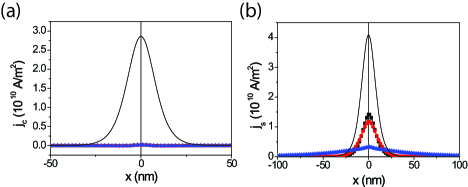
Figure 1: (color online) Results of micromagnetic simulation for (a) charge current and (b) spin current induced by SMF generated from 1D DW oscillator, which is fixed at $x=0$, but rotating with $\omega=10$GHz, in the presence of spin diffusion with $\lambda_{sf}=0.5$nm (black rectangle), $5.0$nm (red circle), and $50$nm (blue triangle). Solid line represents currents without diffusion. Here, DW width is set to be 10nm.

We confirmed our analytic result by comparing it with micromagnetic simulation for a 1D DW oscillator. The result is in Fig. 1. General features are the same as analytic result ; i) charge and spin currents are highly suppressed by spin diffusion, ii) spin current becomes nonlocal, iii) charge current almost vanish independently of diffusion length, and iv) spin current is more suppressed by larger diffusion length.

Now, we generalize the results to higher dimension. In 2D and 3D real spaces, Eqs. (61) and (62) are converted to

$$\mathbf{j}_{e}^{2D} = P\sigma\mathbf{E}_{s}-\frac{P\sigma}{2\pi}\nabla\int d^{2}x^{\prime}\ln\frac{|\mathbf{x}-\mathbf{x}^{\prime}|}{\lambda_{sf}}\nabla^{\prime}\cdot\mathbf{E}_{s},$$ (67a)

$$\mathbf{j}_{e}^{3D} = P\sigma\mathbf{E}_{s}+\frac{P\sigma}{4\pi}\nabla\int d^{3}x^{\prime}\frac{\nabla^{\prime}\cdot\mathbf{E}_{s}}{|\mathbf{x}-\mathbf{x}^{\prime}|},$$ (67b)

and

$$\mathbf{j}_{s}^{2D} = P\mathbf{j}_{e}^{2D}+(1-P^{2})\sigma\mathbf{E}_{s}$$ (68a)

$$+\frac{(1-P^{2})\sigma}{2\pi}\nabla\int d^{2}x^{\prime}K_{0}\left(\frac{|\mathbf{x}-\mathbf{x}^{\prime}|}{\lambda_{sf}}\right)\nabla^{\prime}\cdot\mathbf{E}_{s},$$

$$\mathbf{j}_{s}^{3D} = P\mathbf{j}_{e}^{3D}+(1-P^{2})\sigma\mathbf{E}_{s}$$ (68b)

$$+\frac{(1-P^{2})\sigma}{4\pi}\nabla\int d^{3}x^{\prime}\frac{e^{-|\mathbf{x}-\mathbf{x}^{\prime}|/\lambda_{sf}}}{|\mathbf{x}-\mathbf{x}^{\prime}|}\nabla^{\prime}\cdot\mathbf{E}_{s},$$

respectively. Here, $K_{0}(x)$ is the zeroth order modified Bessel function of the second kind. One can be uncomfortable because $\mathbf{j}_{e}^{2D}$ seems dependent on $\lambda_{sf}$ while Eq. (61) is not. Here $\lambda_{sf}$ is included because the argument of logarithmic function should be dimensionless. In fact, one can easily check that $\mathbf{j}_{e}^{2D}$ does not depend on $\lambda_{sf}$ by using $\ln|\mathbf{x}-\mathbf{x}^{\prime}|/\lambda_{sf}^{\prime}=\ln|\mathbf{x}-\mathbf{x}^{\prime}|/\lambda_{sf}+$(constant) for any positive $\lambda_{sf}^{\prime}$.

From now on, we present only 3D expressions but omit 2D, for simplicity. One can easily obtain 2D expressions by replacing the integral kernels $1/|\mathbf{x}-\mathbf{x}^{\prime}|\rightarrow-2\ln|\mathbf{x}-\mathbf{x}^{\prime}|/\lambda_{sf}$ and $\exp(-|\mathbf{x}-\mathbf{x}^{\prime}|/\lambda_{sf})/|\mathbf{x}-\mathbf{x}^{\prime}|\rightarrow 2K_{0}\left(\frac{|\mathbf{x}-\mathbf{x}^{\prime}|}{\lambda_{sf}}\right)$. The reason why the expressions depend on dimension is nothing but the fact that the inverse Fourier transforms, which give integration kernels, depend on dimension. Hence, essential physics are the same for 2D and 3D except the mathematical expressions of the integration kernels.

Overall features of the spin current in higher dimension is similar to 1D, except for the existence of nonvanishing $P\mathbf{j}_{e}$ term. However, the main feature of $\mathbf{j}_{e}$ is completely different from 1D case. First of all, $\mathbf{j}_{e}$ does not vanish. We argued qualitatively why the charge current vanishes in a 1D system by using chemical potential argument. However, in a higher dimensional system, chemical potential cannot be defined in general since $\mathbf{E}_{s}$ is nonconservative. Note that diffusion current $D^{\uparrow\downarrow}\nabla n^{\uparrow\downarrow}$ is conservative. Note also that nonconservative field cannot be canceled by conservative field. This is why the charge current exists in a higher dimensional system. The nonlocal term in Eq. (67) can be interpreted as Coulomb potential under charge density $-\nabla\cdot\mathbf{E}_{s}$. The canceled part of the charge current is nothing but conservative Coulomb part of $\mathbf{E}_{s}$. Secondly, it is very interesting that Eq. (67) is converted after some algebra to

$$\mathbf{j}_{e}=\frac{P\sigma}{4\pi}\int d^{3}x^{\prime}\frac{\nabla^{\prime}\times\left(\nabla^{\prime}\times\mathbf{E}_{s}\right)}{|\mathbf{x}-\mathbf{x}^{\prime}|}.$$ (69)

Now one can notice the importance of nonconservative part of $\mathbf{E}_{s}$ (nonvanishing $\nabla\times\mathbf{E}_{s}$) and the dependence of this on the charge current. If $\nabla\times\mathbf{E}_{s}$ happens to be zero, the charge current also vanishes, and this is consistent to the chemical potential argument. Lastly, it is also interesting that charge current does not depend on diffusion length. This is qualitatively understandable from the fact that the effect of $\mathbf{E}_{s}$ is maximally canceled by diffusion current in small spin-flip time regime, regardless of spin diffusion length. Here, maximal cancelation is slightly different from perfect cancelation in 1D case in the sense that the (conservative) diffusion current cannot cancel $P\sigma\mathbf{E}_{s}$ perfectly in principle.

It might be ambiguous what the “conservative part” of a vector field is mathematically. Helmholtz’s theorem guarantees that a spatially localized vector field can be uniquely decomposed into conservative (curl-free) part and solenoidal (divergence-free) part. Note that the second term in Eq. (67) is exactly the same as the formula of (negative of) conservative part of the Helmholtz decomposition. Note also that the resulting total current [Eq. (69)] is divergence-free. Therefore, the charge diffusion current and total charge current are respectively given by conservative part and solenoidal part of Helmholtz decomposition. One shall see in Sec. V that this claim is generally valid for arbitrary boundary conditions.

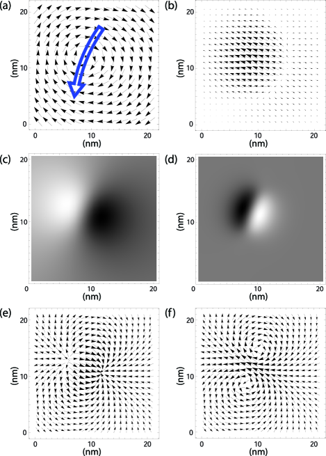
Figure 2: (color online) Results of the micromagnetic simulation for vortex resonant oscillation in 2D thin film. Here, the vortex core size is about 5nm, the resonant frequency is 605.5MHz, and $P=P_{n}=0.7$. The size of arrows are log-scaled (size $\propto$ ln(1+norm)). (a) Magnetization profile at the time when all calculation was performed. The blue arrow denotes the direction of vortex core motion. (b) SMF. (c) Accumulated charge density $-e\Delta n_{e}$ (divided by $\sigma\tau_{sf}/\lambda_{sf}^{2}$). The maximum value (white) is $1.39\times 10^{-5}$V and the minimum value (black) is $-1.62\times 10^{-5}$V. (d) $\nabla\cdot\mathbf{E}_{s}$. The maximum value (white) is $8.43\times 10^{10}$V/m² and the minimum value (black) is $-7.42\times 10^{10}$V/m². (e) Charge diffusion current, which is the conservative part of SMF. (f) Total charge current, which is the solenoidal part of SMF.

To understand the maximal cancelation of the charge current qualitatively, it would be very helpful to visualize the Helmholtz decomposition of the charge current. We performed a micromagnetic simulation for vortex resonant oscillation in 2D thin film. When the vortex DW wall [Fig. 2(a)] moves along the blue arrow, SMF is generated as shown in Fig. 2(b). The spatial dependence of SMF induces charge accumulation as shown in Fig. 2(c). Due to the charge accumulation, charge diffusion current is generated as shown in Fig. 2(e). Figure 2(e) can be qualitatively understood by Fig. 2(d). Recall that the diffusion current is given by Coulomb field generated by charge density $-\nabla\cdot\mathbf{E}_{s}$. Thus, dipole-like nature of the charge density $-\nabla\cdot\mathbf{E}_{s}$ [Fig. 2(d)] implies dipole-like field [Fig. 2(e)]. Summing up Figs. 2(b) and 2(e), one obtains total current as Fig. 2(f). Note that the total current is definitely nonconservative (has finite curl). It is interesting that Fig. 2(f) is similar to magnetic field generated by two separate conducting wires. This infers the solenoidal nature of the total charge current. It is very interesting that total charge current behaves as magnetic field rather than electric field.

III.3 Magnetization dynamics and nonlocal damping tensor

It is also important to see how the magnetization dynamics is changed by our result. By analogue of Ref. Zhang04PRL , it is obvious that the modified LLG equation is described by Eq. (1), in which Eq. (68) are added to $\mathbf{j}_{s}$ terms, rather than Eq. (49). However, there exist two nontrivial features in the modified LLG equation.

The first one is spatial dependence of $\gamma$ and $\alpha$. It is important to notice that $\gamma$ and $\alpha$ in Eq. (1) are renormalized parameters Zhang04PRL ,

$$\gamma = \gamma_{0}\left(1+\frac{n_{s}\mu_{B}}{M_{s}}\frac{1}{1+\beta^{2}}\right)^{-1},$$ (70)

$$\alpha = \frac{\gamma_{0}}{\gamma}\left(\alpha_{0}+\beta\frac{n_{s}\mu_{B}}{M_{s}}\frac{1}{1+\beta^{2}}\right),$$ (71)

where $\gamma_{0}$ and $\alpha_{0}$ are original parameters of the system. There has not been any problem of this renormalization without spin accumulation, but $n_{s}$ is no longer constant in the presence of spin accumulation. Hence, $\gamma$ and $\alpha$ cannot be a simple constant in principle. At this stage, it is more convenient to write down LLG equation without parameter renormalization,

$$\left(1+\frac{1}{1+\beta^{2}}\frac{n_{s}\mu_{B}}{M_{s}}\right)\frac{\partial\mathbf{M}}{\partial t}=-\gamma_{0}\mathbf{M}\times\mathbf{H}_{eff}$$

$$+\left(1+\frac{\beta}{\alpha_{0}}\frac{1}{1+\beta^{2}}\frac{n_{s}\mu_{B}}{M_{s}}\right)\frac{\alpha_{0}}{M_{s}}\mathbf{M}\times\frac{\partial\mathbf{M}}{\partial t}$$

$$+\frac{\mu_{B}}{eM_{s}}(\mathbf{j}_{s}\cdot\nabla)\mathbf{M}-\frac{\beta\mu_{B}}{eM_{s}^{2}}\mathbf{M}\times(\mathbf{j}_{s}\cdot\nabla)\mathbf{M}.$$ (72)

In fact, the effect of $n_{s}$ variation is small. Note that $n_{s}\mu_{B}/M_{s}=(n_{0}^{\uparrow}-n_{0}^{\downarrow})\mu_{B}/M_{s}\times\Delta n_{s}/(n_{0}^{\uparrow}-n_{0}^{\downarrow})$. Here, the first factor is of the order of $10^{-2}$ and the second factor is first order in SMF. Then, the effect should be very small compared to ordinary first order effect of SMF. In addition, one shall see in Sec. IV, that symmetry can reduce the effect of $\Delta n_{s}$ in collective coordinate level. In the case, the effect of $\Delta n_{s}$ vanishes through odd function integration.

The next one is effective damping constant. Without applied electric field, the modified LLG equation is obtained by taking Gilbert damping as a damping tensor like Eq. (4). Then, it is interesting to see how the damping tensor is generalized by spin diffusion effect. In the presence of spin diffusion, local damping tensor $\mathcal{D}_{ij}$ becomes nonlocal damping tensor $\mathcal{D}_{ij}(\mathbf{x},\mathbf{x}^{\prime})$. By using Eq. (68), it turns out that the damping tensor in Eq. (4) is modified as

$$\mathcal{D}_{ij}(x,x^{\prime}) = \alpha\delta_{ij}\delta(x-x^{\prime})+\frac{(1-P^{2})\eta}{M_{s}^{4}}\frac{e^{-|x-x^{\prime}|/\lambda_{sf}}}{2\lambda_{sf}}$$ (73)

$$\times(\mathbf{M}\times\partial_{x}\mathbf{M})_{i}(\mathbf{M}^{\prime}\times\partial_{x}\mathbf{M}^{\prime})_{j},$$

for 1D and

$$\mathcal{D}_{ij}(\mathbf{x},\mathbf{x}^{\prime}) = \alpha\delta_{ij}\delta(\mathbf{x}-\mathbf{x}^{\prime})+\frac{\eta}{\sigma M_{s}^{4}}S_{kl}(\mathbf{x},\mathbf{x}^{\prime})$$ (74)

$$\times(\mathbf{M}\times\partial_{k}\mathbf{M})_{i}(\mathbf{M}^{\prime}\times\partial_{l}\mathbf{M}^{\prime})_{j},$$

$$\mathcal{S}_{ij}(\mathbf{x},\mathbf{x}^{\prime}) = \sigma\delta_{ij}\delta(\mathbf{x}-\mathbf{x}^{\prime})+\frac{P^{2}\sigma}{4\pi}\partial_{i}\partial_{j}\frac{1}{|\mathbf{x}-\mathbf{x}^{\prime}|}$$ (75)

$$+\frac{(1-P^{2})\sigma}{4\pi}\partial_{i}\partial_{j}\frac{e^{-|\mathbf{x}-\mathbf{x}^{\prime}|/\lambda_{sf}}}{|\mathbf{x}-\mathbf{x}^{\prime}|}.$$

for 3D. Here, $\mathbf{M}^{\prime}=\mathbf{M}(\mathbf{x}^{\prime},t)$ and $\cdot$ is redefined as inner product with respect to both coordinate basis and spatial basis,

$$\left[\mathcal{D}\cdot\mathbf{f}(\mathbf{x})\right]_{i}=\sum_{j}\int d^{d}x^{\prime}\mathcal{D}_{ij}(\mathbf{x},\mathbf{x}^{\prime})f_{j}(\mathbf{x}^{\prime}),$$ (76)

for a vector field $\mathbf{f}$. As a passing remark, the tensor $\mathcal{D}$ is indeed a damping tensor in the sense that it decreases total magnetic energy. It can be demonstrated by showing energy dissipation is negative,

$$\frac{dE}{dt}=-\int\left(\mathbf{H}_{eff}\cdot\frac{\partial\mathbf{M}}{\partial t}\right)d^{d}x<0.$$ (77)

The mathematical details related to Eqs. (73)-(77) are in Appendix C.

IV Example : Domain wall motion

In this section, we apply our theory to 1D DW motion. We find equation of motion of collective coordinates $(X(t),\phi(t))$ of tail-to-tail transverse DW. Here, $X(t)$ is DW position and $\phi(t)$ is tilting angle. Mathematical details of obtaining the collective coordinate equation is described in Appendix D.

Without SMF, DW motion is described by Thiele73PRL ; Jung08APL ; Ryu09JAP ; Malozemoff79 ; Schryer74JAP ; Tatara06JPS ; Tatara04PRL

$$-\frac{\partial\phi}{\partial t}+\frac{\alpha}{\lambda}\frac{\partial X}{\partial t} = -\frac{\beta b_{J}^{0}}{\lambda},$$ (78)

$$\frac{1}{\lambda}\frac{\partial X}{\partial t}+\alpha\frac{\partial\phi}{\partial t} = -\frac{b_{J}^{0}}{\lambda}-\frac{\gamma K_{d}}{M_{s}}\sin 2\phi,$$ (79)

where $b_{J}^{0}=Pj\mu_{B}/eM_{s}$ for applied current $j$, $K_{d}$ represents dipole field integration, and $\lambda$ is DW width. In the presence of SMF, Eqs. (78) and (79) are modified as Kim11CAP

$$-\frac{\partial\phi}{\partial t}+\frac{\alpha}{\lambda}\frac{\partial X}{\partial t} = -\frac{\beta b_{J}^{0}}{\lambda}-\frac{2\beta\eta}{3\lambda^{2}}\frac{\partial\phi}{\partial t},$$ (80)

$$\frac{1}{\lambda}\frac{\partial X}{\partial t}+\alpha\frac{\partial\phi}{\partial t} = -\frac{b_{J}^{0}}{\lambda}-\frac{2\eta}{3\lambda^{2}}\frac{\partial\phi}{\partial t}-\frac{\gamma K_{d}}{M_{s}}\sin 2\phi.$$ (81)

One can expect that the effect of $\eta$ will be suppressed by spin diffusion, so a renormalized parameter $\tilde{\eta}$ will replace $\eta$. Thus, the expected equations of motion are

$$-\frac{\partial\phi}{\partial t}+\frac{\alpha}{\lambda}\frac{\partial X}{\partial t} = -\frac{\beta b_{J}^{0}}{\lambda}-\frac{2\beta\tilde{\eta}}{3\lambda^{2}}\frac{\partial\phi}{\partial t},$$ (82)

$$\frac{1}{\lambda}\frac{\partial X}{\partial t}+\alpha\frac{\partial\phi}{\partial t} = -\frac{b_{J}^{0}}{\lambda}-\frac{2\tilde{\eta}}{3\lambda^{2}}\frac{\partial\phi}{\partial t}-\frac{\gamma K_{d}}{M_{s}}\sin 2\phi.$$ (83)

As described in Appendix D, it turns out that Eqs. (82) and (83) are indeed valid, and the renormalized SMF parameter is given by

$$\tilde{\eta} = (1-P^{2})F(\zeta)\eta,$$ (84)

$$F(\zeta) = -\frac{3}{2}\zeta-\frac{3}{2}\zeta^{2}+\frac{3}{4}\zeta^{3}\left.\left(\frac{\Gamma^{\prime}(z)}{\Gamma(z)}\right)\right|_{z=\frac{\zeta}{2}},$$ (85)

where $\zeta=\lambda/\lambda_{sf}$ and $\Gamma(z)$ is the Gamma function.

The renormalization is largely dependent on relative magnitude of DW width and spin diffusion length. The asymptotic behavior of the function $F$ is given by

$$F(\zeta)=\left\{\begin{array}[]{cc}\frac{3}{2}\zeta-\frac{3}{2}\zeta^{2}+\frac{\pi^{2}\zeta^{3}}{8}+\mathcal{O}(\zeta^{4})&\zeta\ll 1,\\ 1-\frac{4}{5\zeta^{2}}+\mathcal{O}(\zeta^{-4})&\zeta\gg 1.\end{array}\right.$$ (86)

For $\lambda\ll\lambda_{sf}$, Eqs. (80) and (81) are reproduced except $(1-P^{2})$ factor which should exist as already discussed. For $\lambda\gg\lambda_{sf}$, the effect is highly suppressed by spin diffusion, so the overall effect of SMF goes as $\frac{1}{\lambda\lambda_{sf}}$ rather than $\frac{1}{\lambda^{2}}$.

V Further generalizations

V.1 Extended electric field - general boundary condition

In the case that the magnetization dynamics is generated by applied electric field, the electric field is no longer localized. Hence, it is necessary to generalize our theory to non-localized electric field ; $\mathbf{E}_{s}$ does not vanish at $|\mathbf{x}|\rightarrow\infty$. In this case, $\tilde{\mathcal{E}}$ does not give well-defined Fourier transform, but includes delta function parts. Furthermore, in order to obtain Eq. (69), one obtains additional boundary terms when integrating Eq. (67) by parts. Hence, the charge current may not be canceled by the diffusion current even if the electric field is conservative.

The problem can be treated by Green’s function method with given boundary condition, as described in the last part of this section. However, it is hard to catch the physical meaning, so we present more intuitive analysis for this case. It is very convenient to use the linearity of our theory. Suppose $\mathbf{E}^{\uparrow\downarrow}$ can be decomposed into two components $\mathbf{E}^{\uparrow\downarrow}=\mathbf{E}_{1}^{\uparrow\downarrow}+\mathbf{E}_{2}^{\uparrow\downarrow}$. Then, since Eqs. (13) and (23) are linear, the current $\mathbf{j}^{\uparrow\downarrow}$ can also be decomposed into two components $\mathbf{j}^{\uparrow\downarrow}=\mathbf{j}_{1}^{\uparrow\downarrow}+\mathbf{j}_{2}^{\uparrow\downarrow}$, where $\mathbf{j}_{i}^{\uparrow\downarrow}$ is the current generated by $\mathbf{E}_{i}$.

To take advantage of this linearity, we decompose $\mathbf{E}$ into three components as follows; any vector field $\mathbf{E}$ can be uniquely decomposed into irrotational part $\mathbf{E}_{1}$, solenoidal part $\mathbf{E}_{2}$, and boundary part $\mathbf{E}_{3}$,

$$\mathbf{E}^{\uparrow\downarrow}=\mathbf{E}_{1}^{\uparrow\downarrow}+\mathbf{E}_{2}^{\uparrow\downarrow}+\mathbf{E}_{3}^{\uparrow\downarrow},$$ (87)

$$\nabla\cdot\mathbf{E}_{1}^{\uparrow\downarrow}\neq 0,~{}\nabla\times\mathbf{E}_{1}^{\uparrow\downarrow}=0,~{}\mathbf{n}\cdot\mathbf{E}_{1}^{\uparrow\downarrow}|_{\mathbf{x}\in\partial}=0,$$ (88)

$$\nabla\cdot\mathbf{E}_{2}^{\uparrow\downarrow}=0,~{}\nabla\times\mathbf{E}_{2}^{\uparrow\downarrow}\neq 0,~{}\mathbf{n}\cdot\mathbf{E}_{2}^{\uparrow\downarrow}|_{\mathbf{x}\in\partial}=0,$$ (89)

$$\nabla\cdot\mathbf{E}_{3}^{\uparrow\downarrow}=0,~{}\nabla\times\mathbf{E}_{3}^{\uparrow\downarrow}=0,~{}\mathbf{n}\cdot\mathbf{E}_{3}^{\uparrow\downarrow}|_{\mathbf{x}\in\partial}\neq 0.$$ (90)

Here, $\partial$ means boundary and $\mathbf{n}$ denotes a normal unit vector perpendicular to the boundary. From given $\mathbf{E}^{\uparrow\downarrow}$, one can obtain $\mathbf{E}_{3}^{\uparrow\downarrow}$ by solving Laplace equation with Neumann boundary condition and $\mathbf{E}_{1,2}^{\uparrow\downarrow}$ by Helmholtz’s theorem. As previously mentioned, our result [Eq. (69)] indicates that the conservative source part $\mathbf{E}_{1}^{\uparrow\downarrow}$ cannot contribute to the charge current while the nonconservative solenoidal part $\mathbf{E}_{2}^{\uparrow\downarrow}$ can give rise to a nonvanishing contribution $\sigma^{\uparrow}\mathbf{E}_{2}^{\uparrow}+\sigma^{\downarrow}\mathbf{E}_{2}^{\downarrow}$. [Eq. (67) or Eq. (113) for general boundary condition]

In the presence of nonvanishing boundary condition, it is important to investigate the effect of $\mathbf{E}_{3}^{\uparrow\downarrow}$ to the spin accumulation. Fortunately, the source term of Eq. (13) depends on the divergence of $\mathbf{E}_{s}^{\uparrow\downarrow}$ only. Hence, $\mathbf{E}_{3}^{\uparrow\downarrow}$ cannot contribute to the spin accumulation since $\nabla\cdot\mathbf{E}_{3}^{\uparrow\downarrow}=0$. Therefore, $\mathbf{E}_{3}^{\uparrow\downarrow}$ can only contribute to the currents via the first term in Eq. (23). Consequently, the expressions of charge and spin current should be $\sigma^{\uparrow}\mathbf{E}_{3}^{\uparrow}\pm\sigma^{\downarrow}\mathbf{E}_{3}^{\downarrow}$ added to Eqs. (67) and (68) (or Eqs. (63) and (64)).

It can be a good example that a constant spin independent electric field $\mathbf{E}_{app}=E_{app}\hat{x}$ is applied in a 1D wire. In this case, $\mathbf{E}_{3}^{\uparrow\downarrow}=E_{app}\hat{x}$. Hence, the charge and spin current should be $\sigma^{\uparrow}E_{app}\pm\sigma^{\downarrow}E_{app}$ added to Eqs. (63) and (64), so

$$j_{e} = \sigma E_{app},$$ (91)

$$j_{s} = P\sigma E_{app}+(1-P^{2})\int dx^{\prime}\frac{e^{-|x-x^{\prime}|/\lambda_{sf}}}{2\lambda_{sf}}\sigma E_{s}(x^{\prime},t).$$ (92)

In this case, the charge current is not canceled by diffusion current, but only charge current generated by SMF (which is spatially localized) is canceled.

V.2 Charge neutrality and other spin independent potentials

There is another important physical consequence of spin accumulation we have ignored. This is Coulomb potential of accumulated electrons. Since Coulomb potential is in general strong, electron tends to make local charge neutral. Hence, giving a charge neutrality constraint,

$$\Delta n^{\uparrow}+\Delta n^{\downarrow}=0$$ (93)

is a good approximation. To do this, it is convenient to introduce charge neutrality potential $V_{c}$ and replace $\mathbf{E}_{s}^{\uparrow\downarrow}\rightarrow\mathbf{E}_{s}^{\uparrow\downarrow}-\nabla V_{c}$ as suggested in Ref. Tserkovnyak08PRB . Then, the solution of the spin drift-diffusion equation [Eq. (37)] is modified by

$$\left(\begin{array}[]{c}\Delta\tilde{n}^{\uparrow}\\ \Delta\tilde{n}^{\downarrow}\\ \end{array}\right)=\frac{\tau_{sf}}{e}\Omega^{-1}\left(\begin{array}[]{cc}\sigma^{\uparrow}&0\\ 0&\sigma^{\downarrow}\\ \end{array}\right)i\mathbf{k}\cdot\left(\begin{array}[]{c}\tilde{\mathbf{E}}_{s}-i\mathbf{k}\tilde{V}_{c}\\ -\tilde{\mathbf{E}}_{s}-i\mathbf{k}\tilde{V}_{c}\\ \end{array}\right),$$ (94)

where $V_{c}$ is found self-consistently to satisfy Eq. (93). After straightforward algebra, one obtains charge neutrality potential in terms of $\mathbf{E}_{s}$,

$$\tilde{V}_{c}(\mathbf{k},t) = -\frac{Pi\mathbf{k}\cdot\tilde{\mathbf{E}}_{s}}{k^{2}}-\frac{(P_{n}-P)i\mathbf{k}\cdot\tilde{\mathbf{E}}_{s}}{k^{2}+\lambda_{sf}^{-2}},$$ (95)

$$V_{c}(\mathbf{x},t) = -\frac{P}{4\pi}\int d^{3}x^{\prime}\frac{1}{|\mathbf{x}-\mathbf{x}^{\prime}|}\nabla\cdot\mathbf{E}_{s}$$ (96)

$$-\frac{P_{n}-P}{4\pi}\int\frac{e^{-|\mathbf{x}-\mathbf{x}^{\prime}|/\lambda_{sf}}}{|\mathbf{x}-\mathbf{x}^{\prime}|}\nabla\cdot\mathbf{E}_{s}.$$

The effect of this potential is twofold. Firstly, $V_{c}$ gives additional electrical current $-\sigma^{\uparrow\downarrow}\nabla V_{c}$. In $k$-space,

$$\Delta\tilde{\mathbf{j}}_{c}^{\uparrow}(\mathbf{k},t) = -\sigma^{\uparrow}i\mathbf{k}V_{c},$$ (97)

$$\Delta\tilde{\mathbf{j}}_{c}^{\downarrow}(\mathbf{k},t) = -\sigma^{\downarrow}i\mathbf{k}V_{c}.$$ (98)

Secondly, $V_{c}$ affects diffusion current through $\nabla n^{\uparrow\downarrow}$. After some algebra, one obtains

$$\left(\begin{array}[]{c}\Delta\tilde{\mathbf{j}}_{D}^{\uparrow}\\ \Delta\tilde{\mathbf{j}}_{D}^{\downarrow}\\ \end{array}\right) = i\mathbf{k}\left(\begin{array}[]{cc}\lambda_{sf}^{\uparrow 2}&0\\ 0&\lambda_{sf}^{\downarrow 2}\\ \end{array}\right)\Omega^{-1}\left(\begin{array}[]{cc}\sigma^{\uparrow}&0\\ 0&\sigma^{\downarrow}\\ \end{array}\right)\left(\begin{array}[]{c}k^{2}V_{c}\\ k^{2}V_{c}\\ \end{array}\right)$$ (107)

$$= i\mathbf{k}V_{c}\left(\begin{array}[]{c}\sigma^{\uparrow}\\ \sigma^{\downarrow}\\ \end{array}\right),$$ (110)

which exactly cancels Eqs. (97) and (98). Hence, there are no additional charge and spin currents attributed to $V_{s}$.

It is very interesting that one does not need to assume any specific form of $V_{c}$ to reach Eq. (110). The mathematical origin of the exact cancelation is that the additional force is conservative (described by $i\mathbf{k}\times$(scalar)) and spin independent. A spin independent potential generates additional current, but spin accumulation adjusts fast to make diffusion current cancel it. Of course, the modified spin accumulation $n^{\uparrow\downarrow}$ affects LLG equation by Eq. (72), but we claimed that this is ignorable. Consequently, any spin independent potential cannot modify the main features of our result. As another side remark, this cancelation can be verified for exact Coulomb potential even without using the charge neutrality approximation Eqs. (93)-(96).

V.3 Arbitrary boundary

Since SMF is usually strongly localized, we have considered an infinite boundary problem. However, for a finite system, the expression of the charge and spin currents should be slightly modified. Note that the key part of our theory is to find real space expression of $\Omega^{-1}$. (See Eq. (37)). In real space, $\Omega$ is a differential operator,

$$\Omega_{real}=\left(\begin{array}[]{cc}-\lambda_{sf}^{\uparrow 2}\nabla^{2}+\frac{n_{0}^{\downarrow}}{n_{0}^{\uparrow}+n_{0}^{\downarrow}}&-\frac{n_{0}^{\uparrow}}{n_{0}^{\uparrow}+n_{0}^{\downarrow}}\\ -\frac{n_{0}^{\downarrow}}{n_{0}^{\uparrow}+n_{0}^{\downarrow}}&-\lambda_{sf}^{\downarrow 2}\nabla^{2}+\frac{n_{0}^{\uparrow}}{n_{0}^{\uparrow}+n_{0}^{\downarrow}}\\ \end{array}\right).$$ (111)

Hence, the problem is to find the inverse operator, i.e., the Green’s function corresponding $\Omega_{real}$ at the given geometry.

In order to find the Green’s function of $\Omega_{real}$, one can get a hint from Eq. (40). Firstly, let $G_{L}(\mathbf{x},\mathbf{x}^{\prime})$ and $G_{H}(\mathbf{x},\mathbf{x}^{\prime})$ be respectively the Green’s function corresponding Laplacian $\nabla^{2}$ and modified Helmholtz operator $\nabla^{2}-\lambda_{sf}^{-2}$ for the given geometry. In order to obtain the Green’s function, it is plausible to replace $1/k^{2}\rightarrow-G_{L}(\mathbf{x},\mathbf{x}^{\prime})$ and $1/(k^{2}+\lambda_{sf}^{-2})\rightarrow-G_{H}(\mathbf{x},\mathbf{x}^{\prime})$ in Eq. (40). Then, one obtains

$$G_{\Omega}(\mathbf{x},\mathbf{x}^{\prime})=-\frac{1}{\sigma}\left(\begin{array}[]{cc}\frac{\sigma^{\uparrow}G_{L}+\sigma^{\downarrow}G_{H}}{\lambda_{sf}^{\uparrow 2}}&\frac{\sigma^{\uparrow}G_{L}-\sigma^{\uparrow}G_{H}}{\lambda_{sf}^{\uparrow 2}}\\ \frac{\sigma^{\downarrow}G_{L}-\sigma^{\downarrow}G_{H}}{\lambda_{sf}^{\downarrow 2}}&\frac{\sigma^{\downarrow}G_{L}+\sigma^{\uparrow}G_{H}}{\lambda_{sf}^{\downarrow 2}}\\ \end{array}\right).$$ (112)

One can verify this is indeed the Green’s function of $\Omega_{real}$ by showing $\Omega_{real}G_{\Omega}=\delta(\mathbf{x}-\mathbf{x}^{\prime})$. Then, one straightforwardly concludes that the generalized expressions of charge and spin current [Eqs. (67)-(68)] are given by

$$\mathbf{j}_{e} = P\sigma\mathbf{E}_{s}-P\sigma\nabla\int d^{d}x^{\prime}G_{L}(\mathbf{x},\mathbf{x}^{\prime})\nabla^{\prime}\cdot\mathbf{E}_{s},$$ (113)

$$\mathbf{j}_{s} = P\mathbf{j}_{e}+(1-P^{2})\sigma\mathbf{E}_{s}$$ (114)

$$-(1-P^{2})\sigma\nabla\int d^{d}x^{\prime}G_{H}(\mathbf{x},\mathbf{x}^{\prime})\nabla^{\prime}\cdot\mathbf{E}_{s}.$$

For infinite boundary with vanishing boundary condition, $4\pi G_{L}=-1/|\mathbf{x}-\mathbf{x}^{\prime}|$ and $4\pi G_{H}=-e^{-|\mathbf{x}-\mathbf{x}^{\prime}|/\lambda_{sf}}/|\mathbf{x}-\mathbf{x}^{\prime}|$, so Eqs. (67)-(68) are reproduced.

VI Conclusion

By constructing spin drift-diffusion equation from the equation of motion of conduction electrons, we studied the effect of SMF in the presence of spin accumulation, spin diffusion and spin flip scattering, which were ignored Zhang09PRL or considered only in 1D Zhang10PRB in previous theories. It turns out that, in realistic regime, the conservative part of charge current is canceled by diffusion current, and spin current becomes nonlocal. Consequently, the magnetization dynamics is affected by nonlocal Gilbert damping tensor, instead of the previously reported (local) Gilbert damping tensor. By calculating spin-transfer torque generated by nonlocal spin current, we obtained the explicit expressions of the nonlocal Gilbert damping tensor.

Different from the previous work focusing on 1D Zhang10PRB , we also obtained the results for 2D and 3D as well as 1D. In a 1D system, the results of the previous theory are reproduced. It turns out that Einstein’s relation prevents the existence of charge current, but for parameter sets which do not satisfy the Einstein’s relation, the charge current can be induced by the spin motive force. After generalizing the results to higher dimension, we find that the nonconservative part of SMF plays an important role in charge and spin currents.

As an illustration of suppression of the effect of SMF, we demonstrated equations of motion of collective coordinate of 1D current-induced DW motion. We found that spin diffusion renormalizes SMF depending on the relative magnitude of DW width and spin diffusion length.

We also investigated the system under spatially extended (non-localized) electric field. In this case, it turns out that the spatially extended part of the electric field can contribute to the charge current even though it is conservative. However, the existence of spatially extended part of the electric field cannot alter the result that the charge current generated by (localized) SMF cannot include conservative part.

Our result is solid in the sense that our principal results are not changed by any spin independent potential. A spin independent potential modifies current via additional electric field, but spin density rapidly adjusts to make diffusion current cancel it. Consequently, a spin independent potential can modify spin density, but not current.

Appendix A Absence of Time Variation of Equilibrium Number Density

In this section, we show that $e^{-\Omega t/\tau_{sf}}\tilde{\mathcal{N}}(\mathbf{k},0)$ does not have time dependence, where $\Omega$ is given by Eq. (31) and $\tilde{\mathcal{N}}(\mathbf{k},0)=(2\pi)^{d/2}\delta(\mathbf{k})(n_{0}^{\uparrow}~{}n_{0}^{\downarrow})^{T}$. It suffices to calculate $e^{-\Omega t/\tau_{sf}}$ at $k=0$ because of $\delta(\mathbf{k})$ factor. It is easy to show that $\Omega$ is idempotent for $k=0$. In other words, $\Omega^{n}|_{k=0}=\Omega|_{k=0}$. Then, for $k=0$,

$$e^{-\Omega t/\tau_{sf}} = \sum_{n=0}^{\infty}\frac{\Omega^{n}}{n!}\left(-\frac{t}{\tau_{sf}}\right)^{n}=I+\sum_{n=1}^{\infty}\frac{\Omega}{n!}\left(-\frac{t}{\tau_{sf}}\right)^{n},$$ (115)

$$= I+\Omega(e^{-t/\tau_{sf}}-1).$$

where $I$ is the identity matrix. Since

$$\Omega\tilde{\mathcal{N}}(\mathbf{k},0)=(2\pi)^{d/2}\delta(\mathbf{k})\Omega\left(\begin{array}[]{c}n_{0}^{\uparrow}\\ n_{0}^{\downarrow}\\ \end{array}\right)=0$$ (116)

the second term of Eq. (115) vanishes after applied to $\tilde{\mathcal{N}}(\mathbf{k},0)$. Finally, one obtains $e^{-\Omega t/\tau_{sf}}\tilde{\mathcal{N}}(\mathbf{k},0)=\tilde{\mathcal{N}}(\mathbf{k},0)$.

Note that the result is obtained without the approximation that $\tau_{sf}$ is small.

Appendix B Derivation of Eq. (36)

The idea is based on the delta sequence

$$\lim_{n\rightarrow\infty}ne^{-nt}\Theta(t)=\delta(t),$$ (117)

for natural number $n$. This can be generalized as

$$\lim_{u\rightarrow\infty}ne^{-uzt}\Theta(t)=\delta(t),$$ (118)

where $z$ is a complex number satisfying $\Re[z]>0$. This generalization is obvious in that $uze^{-uzt}$ is localized at $t=0$ and $\int_{-\infty}^{\infty}uze^{-uzt}\Theta(t)dt=1$.

We now generalize this relation to matrices. For a diagonalizable matrix $M$ with eigenvalues $\lambda_{i}$ satisfying $\Re[\lambda_{i}]>0$, we claim that

$$\lim_{u\rightarrow\infty}uMe^{-uMt}\Theta(t)=\delta(t)I.$$ (119)

The proof is simple. Since $M$ is diagonalizable, one can write

$$uM=Q\left(\begin{array}[]{ccc}u\lambda_{1}&0&\cdots\\ 0&u\lambda_{2}&\cdots\\ \vdots&\vdots&\ddots\\ \end{array}\right)Q^{-1},$$ (120)

for some $Q$. Then

$$uMe^{-uMx}\Theta(x)$$

$$=Q\left(\begin{array}[]{ccc}u\lambda_{1}e^{-u\lambda_{1}}\Theta(x)&0&\cdots\\ 0&u\lambda_{2}e^{-u\lambda_{2}}\Theta(x)&\cdots\\ \vdots&\vdots&\ddots\\ \end{array}\right)Q^{-1}$$ (124)

$$\rightarrow Q\left(\begin{array}[]{ccc}\delta(x)&0&\cdots\\ 0&\delta(x)&\cdots\\ \vdots&\vdots&\ddots\\ \end{array}\right)Q^{-1}=\delta(x)I,$$ (128)

as $u\rightarrow\infty$.

By taking $M=\Omega$ and $u=1/\tau_{sf}$,

$$\lim_{\tau_{sf}\rightarrow+0}\frac{\Omega}{\tau_{sf}}e^{-\Omega t/\tau_{sf}}\Theta(t)=\delta(t)I,$$ (129)

so, for small $\tau_{sf}$,

$$\frac{\Omega}{\tau_{sf}}e^{-\Omega t/\tau_{sf}}\Theta(t)\approx\delta(t)I,$$ (130)

which is exactly Eq. (36).

As a passing remark, one should check that the real parts of eigenvalues of $\Omega$ are really positive. It is guaranteed by $\mathrm{Tr}~{}\Omega>0$ and $\det\Omega>0$ for any nonzero $\mathbf{k}$. However, the approximation Eq. (36) makes singularity at $\mathbf{k}=0$. Fortunately, this singularity is removed by $i\mathbf{k}$ factor in Eq. (35).

Appendix C Nonlocal damping tensor and energy dissipation

C.1 1D damping tensor

Starting from

$$j_{s} = (1-P^{2})\int dx^{\prime}\frac{e^{-|x-x^{\prime}|/\lambda_{sf}}}{2\lambda_{sf}}\sigma E_{s}(x^{\prime},t),$$ (131)

$$E_{s} = \frac{\hbar}{2eM_{s}^{3}}\partial_{t}\mathbf{M}\cdot(\partial_{x}\mathbf{M}\times\mathbf{M}),$$ (132)

spin-transfer torque driven by SMF is given by

$$\frac{\mu_{B}}{eM_{s}}j_{s}\partial_{x}\mathbf{M} = (1-P^{2})\frac{\eta}{M_{s}^{3}}\partial_{x}\mathbf{M}$$ (133)

$$\times\int dx^{\prime}\frac{e^{-|x-x^{\prime}|/\lambda_{sf}}}{2\lambda_{sf}}\partial_{t}\mathbf{M}^{\prime}\cdot(\partial_{x}\mathbf{M}^{\prime}\times\mathbf{M}^{\prime})$$

$$= \frac{\mathbf{M}}{M_{s}}\times\int dx^{\prime}\left[(1-P^{2})\frac{\eta}{M_{s}^{4}}\frac{e^{-|x-x^{\prime}|/\lambda_{sf}}}{2\lambda_{sf}}\right.$$

$$\left.(\mathbf{M}\times\partial_{x}\mathbf{M})(\mathbf{M}^{\prime}\times\partial_{x}\mathbf{M}^{\prime})\right]\cdot\partial_{t}\mathbf{M}^{\prime}.$$

Then, comparing with Eqs. (4) and (76),

$$\mathcal{D}_{ij}(x,x^{\prime}) = \alpha\delta_{ij}\delta(x-x^{\prime})+\frac{(1-P^{2})\eta}{M_{s}^{4}}\frac{e^{-|x-x^{\prime}|/\lambda_{sf}}}{2\lambda_{sf}}$$ (134)

$$\times(\mathbf{M}\times\partial_{x}\mathbf{M})_{i}(\mathbf{M}^{\prime}\times\partial_{x}\mathbf{M}^{\prime})_{j}.$$

It is interesting to note that

$$\lim_{\lambda_{sf}\rightarrow 0}\mathcal{D}_{ij}(x-x^{\prime}) = \delta(x-x^{\prime})\left[\alpha\delta_{ij}+\frac{(1-P^{2})\eta}{M_{s}^{4}}\right.$$ (135)

$$\left.\times(\mathbf{M}\times\partial_{x}\mathbf{M})_{i}(\mathbf{M}\times\partial_{x}\mathbf{M})_{j}\right].$$

This is exactly the previous result Eq. (5) except $(1-P^{2})$ factor, which should exist regardless of diffusion strength.

Now, the remaining step is to calculate energy dissipation. Energy dissipation is calculated by the integration energy density dissipation $-\mathbf{H}_{eff}\cdot\partial_{t}\mathbf{M}$. From now on, the subscription _eff is dropped until this section ends. Energy dissipation by a nonlocal damping tensor $\mathcal{D}$ is given by

$$\frac{dE}{dt} = -\int dx\mathbf{H}\cdot\left[\frac{\mathbf{M}}{M_{s}}\times\mathcal{D}\cdot\partial_{t}\mathbf{M}\right]$$ (136)

$$= \frac{1}{M_{s}}\int dx(\mathbf{M}\times\mathbf{H})\cdot\mathcal{D}\cdot\partial_{t}\mathbf{M}$$

$$\approx -\frac{\gamma}{M_{s}}\int dx(\mathbf{M}\times\mathbf{H})\cdot\mathcal{D}\cdot(\mathbf{M}\times\mathbf{H})$$

$$= -\frac{\gamma}{M_{s}}\iint dxdx^{\prime}(\mathbf{M}\times\mathbf{H})_{i}\mathcal{D}_{ij}(x,x^{\prime})(\mathbf{M}^{\prime}\times\mathbf{H}^{\prime})_{j},$$

up to first order. Here, $\mathbf{H}^{\prime}=\mathbf{H}(\mathbf{x}^{\prime},t)$. The first term in Eq. (134) gives definitely negative $dE/dt$. The second term, which comes from SMF, gives

$$\frac{dE_{SMF}}{dt} = -\frac{(1-P^{2})\eta\gamma}{M_{s}}\iint dxdx^{\prime}(\mathbf{H}\cdot\partial_{x}\mathbf{M})$$ (137)

$$\times\frac{e^{-|x-x^{\prime}|/\lambda_{sf}}}{2\lambda_{sf}}(\mathbf{H}^{\prime}\cdot\partial_{x}\mathbf{M}^{\prime}).$$

In order to show $dE/dt<0$, it is sufficient to show that $\iint dxdx^{\prime}f(x)e^{-a|x-x^{\prime}|}f(x^{\prime})$ is positive for real function $f$. This is verified by Parseval’s relation and convolution theorem of Fourier transform.

$$\iint dxdx^{\prime}f(x)e^{-a|x-x^{\prime}|}f(x^{\prime})$$

$$=\int dxf(x)^{*}\left[\int dx^{\prime}e^{-a|x-x^{\prime}|}f(x^{\prime})\right]$$

$$=\int dk\mathcal{F}[f(x)](k)^{*}\mathcal{F}\left[\int dx^{\prime}e^{-a|x-x^{\prime}|}f(x^{\prime})\right](k)$$

$$=\sqrt{2\pi}\int dk\mathcal{F}[f(x)](k)^{*}\mathcal{F}[e^{-a|x|}](k)\mathcal{F}[f(x)](k)$$

$$=2a\int dk\frac{\left|\mathcal{F}[f(x)](k)\right|^{2}}{k^{2}+a^{2}}>0.$$ (138)

This implies $dE/dt<0$.

C.2 3D damping tensor

From now on, Einstein’s convention is used. Componentwise expressions of spin current and SMF for a 3D system are

$$j_{s,i} = \sigma E_{s,i}+\frac{P^{2}\sigma}{4\pi}\partial_{i}\int d^{3}x^{\prime}\frac{\partial_{j}^{\prime}E_{s,j}}{|\mathbf{x}-\mathbf{x}^{\prime}|}$$ (139)

$$+\frac{(1-P^{2})\sigma}{4\pi}\partial_{i}\int d^{3}x^{\prime}\frac{e^{-|\mathbf{x}-\mathbf{x}^{\prime}|/\lambda_{sf}}}{|\mathbf{x}-\mathbf{x}^{\prime}|}\partial_{j}^{\prime}E_{s,j},$$

$$E_{s,i} = \frac{\hbar}{2eM_{s}^{3}}\partial_{t}\mathbf{M}\cdot(\partial_{i}\mathbf{M}\times\mathbf{M}).$$ (140)

By integrating by parts in order to remove derivatives in front of $E_{s,j}$,

$$j_{s,i} = \sigma E_{s,i}-\frac{P^{2}\sigma}{4\pi}\partial_{i}\int d^{3}x^{\prime}E_{s,j}(\mathbf{x}^{\prime})\partial_{j}^{\prime}\frac{1}{|\mathbf{x}-\mathbf{x}^{\prime}|}$$ (141)

$$-\frac{(1-P^{2})\sigma}{4\pi}\partial_{i}\int d^{3}x^{\prime}E_{s,j}(\mathbf{x}^{\prime})\partial_{j}^{\prime}\frac{e^{-|\mathbf{x}-\mathbf{x}^{\prime}|/\lambda_{sf}}}{|\mathbf{x}-\mathbf{x}^{\prime}|},$$

$$= \sigma E_{s,i}+\frac{P^{2}\sigma}{4\pi}\int d^{3}x^{\prime}E_{s,j}(\mathbf{x}^{\prime})\partial_{i}^{\prime}\partial_{j}^{\prime}\frac{1}{|\mathbf{x}-\mathbf{x}^{\prime}|}$$

$$+\frac{(1-P^{2})\sigma}{4\pi}\int d^{3}x^{\prime}E_{s,j}(\mathbf{x}^{\prime})\partial_{i}^{\prime}\partial_{j}^{\prime}\frac{e^{-|\mathbf{x}-\mathbf{x}^{\prime}|/\lambda_{sf}}}{|\mathbf{x}-\mathbf{x}^{\prime}|}.$$

Here, it is convenient to introduce nonlocal conductivity tensor $\mathcal{S}$,

$$j_{s,i} = \int d^{3}x^{\prime}\mathcal{S}_{ij}(\mathbf{x},\mathbf{x}^{\prime})E_{s,j}(\mathbf{x}^{\prime}),$$ (142)

$$\mathcal{S}_{ij}(\mathbf{x},\mathbf{x}^{\prime}) = \sigma\delta_{ij}\delta(\mathbf{x}-\mathbf{x}^{\prime})+\frac{P^{2}\sigma}{4\pi}\partial_{i}^{\prime}\partial_{j}^{\prime}\frac{1}{|\mathbf{x}-\mathbf{x}^{\prime}|}$$ (143)

$$+\frac{(1-P^{2})\sigma}{4\pi}\partial_{i}^{\prime}\partial_{j}^{\prime}\frac{e^{-|\mathbf{x}-\mathbf{x}^{\prime}|/\lambda_{sf}}}{|\mathbf{x}-\mathbf{x}^{\prime}|}.$$

Now, spin-transfer torque driven by SMF is given by

$$\frac{\mu_{B}}{eM_{s}}(\mathbf{j}_{s}\cdot\nabla)\mathbf{M}$$

$$=\frac{\mu_{B}}{eM_{s}}\partial_{i}\mathbf{M}\int d^{3}x^{\prime}\cdot\mathcal{S}_{ij}(\mathbf{x},\mathbf{x}^{\prime})E_{s,j}(\mathbf{x}^{\prime})$$

$$=\frac{\mathbf{M}}{M_{s}}\times\left[\frac{\eta}{\sigma M_{s}^{4}}(\mathbf{M}\times\partial_{i}\mathbf{M})\right.$$

$$\phantom{=}\left.\times\int d^{3}x^{\prime}\cdot\mathcal{S}_{ij}(\mathbf{x},\mathbf{x}^{\prime})(\mathbf{M}^{\prime}\times\partial_{j}\mathbf{M}^{\prime})\cdot\partial_{t}\mathbf{M}^{\prime}\right].$$ (144)

Hence, the nonlocal damping tensor for 3D is given by

$$\mathcal{D}_{ij}(\mathbf{x},\mathbf{x}^{\prime}) = \alpha\delta_{ij}\delta(\mathbf{x}-\mathbf{x}^{\prime})+\frac{\eta}{\sigma M_{s}^{4}}S_{kl}(\mathbf{x},\mathbf{x}^{\prime})$$ (145)

$$\times(\mathbf{M}\times\partial_{k}\mathbf{M})_{i}(\mathbf{M}^{\prime}\times\partial_{l}\mathbf{M}^{\prime})_{j}.$$

Now, we calculate energy dissipation. This is an analogue of the previous section. After some algebra,

$$\frac{dE_{SMF}}{dt} = -\frac{\gamma\eta}{\sigma M_{s}}\iint d^{3}xd^{3}x^{\prime}\mathcal{S}_{kl}(\mathbf{x},\mathbf{x}^{\prime})$$ (146)

$$\times(\mathbf{H}\cdot\partial_{k}\mathbf{M})(\mathbf{H}^{\prime}\cdot\partial_{l}\mathbf{M}^{\prime}).$$

In order to show $dE_{SMF}/dt<0$, one should verify

$$\iint d^{3}xd^{3}x^{\prime}(\mathbf{H}\cdot\partial_{i}\mathbf{M})\mathcal{S}_{ij}(\mathbf{x},\mathbf{x}^{\prime})(\mathbf{H}^{\prime}\cdot\partial_{j}\mathbf{M}^{\prime})>0.$$ (147)

Note that $\mathcal{S}_{ij}(\mathbf{x},\mathbf{x}^{\prime})$ is a function of $(\mathbf{x}-\mathbf{x}^{\prime})$. It is convenient to write $\mathcal{S}_{ij}=\mathcal{S}_{ij}(\mathbf{x}-\mathbf{x}^{\prime})$ at this stage. Similar to the previous subsection, by using Parseval’s theorem and convolution theorem of Fourier transform,

$$\iint d^{3}xd^{3}x^{\prime}(\mathbf{H}\cdot\partial_{i}\mathbf{M})\mathcal{S}_{ij}(\mathbf{x}-\mathbf{x}^{\prime})(\mathbf{H}^{\prime}\cdot\partial_{j}\mathbf{M}^{\prime})$$

$$=\int d^{3}k\mathcal{F}[\mathbf{H}\cdot\partial_{i}\mathbf{M}](\mathbf{k})^{*}\tilde{\mathcal{S}}_{ij}(\mathbf{k})\mathcal{F}[\mathbf{H}\cdot\partial_{j}\mathbf{M}](\mathbf{k}).$$ (148)

Here, $\tilde{\mathcal{S}}_{ij}(\mathbf{k})$ is given by

$$\tilde{\mathcal{S}}_{ij}(\mathbf{k})=\frac{\sigma}{(2\pi)^{3/2}}\left[\delta_{ij}-P^{2}\frac{k_{i}k_{j}}{k^{2}}-(1-P^{2})\frac{k_{i}k_{j}}{k^{2}+\lambda_{sf}^{-2}}\right].$$ (149)

Note that the integrand in Eq. (148) is an expectation value of $3\times 3$ matrix $\tilde{\mathcal{S}}_{ij}(\mathbf{k})$ with respect to vector $\mathcal{F}[\mathbf{H}\cdot\partial_{i}\mathbf{M}](\mathbf{k})$. Since $\tilde{\mathcal{S}}_{ij}(\mathbf{k})$ is a Hermitian matrix, the integrand is always positive if the eigenvalues of $\tilde{\mathcal{S}}_{ij}(\mathbf{k})$ are positive. Recall that the eigenvalues of matrix $k_{i}k_{j}$ is given by $(0,0,k^{2})$. The corresponding eigenvectors are definitely the eigenvectors of $\tilde{\mathcal{S}}_{ij}(\mathbf{k})$, so the eigenvalues of $\tilde{\mathcal{S}}_{ij}(\mathbf{k})$ is given by $\left(\frac{\sigma}{(2\pi)^{3/2}},\frac{\sigma}{(2\pi)^{3/2}},\frac{\sigma}{(2\pi)^{3/2}}\frac{\lambda_{sf}^{-2}(1-P^{2})}{k^{2}+\lambda_{sf}^{-2}}\right)$, which are all positive. This proves $dE/dt<0$.

Appendix D 1D DW motion in the presence of spin diffusion

D.1 Collective coordinate equation of 1D DW for space-time dependent spin current and spin density

The starting equation is 1D version of Eq. (72).

$$\left(1+\frac{1}{1+\beta^{2}}\frac{n_{s}\mu_{B}}{M_{s}}\right)\frac{\partial\mathbf{M}}{\partial t}=-\gamma_{0}\mathbf{M}\times\mathbf{H}_{eff}$$

$$+\left(1+\frac{\beta}{\alpha_{0}}\frac{1}{1+\beta^{2}}\frac{n_{s}\mu_{B}}{M_{s}}\right)\frac{\alpha_{0}}{M_{s}}\mathbf{M}\times\frac{\partial\mathbf{M}}{\partial t}$$

$$+b_{J}\frac{\partial\mathbf{M}}{\partial x}-\beta b_{J}\frac{\mathbf{M}}{M_{s}}\times\frac{\partial\mathbf{M}}{\partial x},$$ (150)

where $b_{J}=\mu_{B}j_{s}/eM_{s}$. The main difference from the conventional approach is that $b_{J}$ and $n_{s}$ are space-time dependent. The equation is rewritten as

$$\gamma_{0}\mathbf{M}\times\mathbf{H}_{tot}=0,$$ (151)

where

$$\gamma_{0}\mathbf{H}_{tot} = -\left(1+\frac{1}{1+\beta^{2}}\frac{n_{s}\mu_{B}}{M_{s}}\right)\frac{\mathbf{M}}{M_{s}^{2}}\times\frac{\partial\mathbf{M}}{\partial t}+\gamma_{0}\mathbf{H}_{eff}$$ (152)

$$-\left(\alpha_{0}+\frac{\beta}{1+\beta^{2}}\frac{n_{s}\mu_{B}}{M_{s}}\right)\frac{1}{M_{s}}\frac{\partial\mathbf{M}}{\partial t}$$

$$+b_{J}\frac{\mathbf{M}}{M_{s}^{2}}\times\frac{\partial\mathbf{M}}{\partial x}+\frac{\beta b_{J}}{M_{s}}\frac{\partial\mathbf{M}}{\partial x}.$$

We set the effective magnetic field as $\mathbf{H}_{eff}=\frac{2A}{M_{s}^{2}}\frac{\partial^{2}\mathbf{M}}{\partial x^{2}}+\frac{H_{K}M_{x}}{M_{s}}\hat{x}+\mathbf{H}_{d}$, where $A$ and $K_{d}$ represents exchange coupling and anisotropy, and $\mathbf{H}_{d}$ is dipole field. In addition, the magnetization profile is set to be tail-to-tail transverse wall,

$$\mathbf{M} = M_{s}(\cos\theta,\sin\theta\cos\phi,\sin\theta\sin\phi),$$ (153)

$$\sin\theta = \mathrm{sech\,}\left(\frac{x-X(t)}{\lambda}\right),$$ (154)

$$\cos\theta = \tanh\left(\frac{x-X(t)}{\lambda}\right),$$ (155)

$$\phi = \phi(t),$$ (156)

where $X(t)$ is DW position and $\phi(t)$ is tilting angle.

Note that Eq. (151) implies $\mathbf{H}_{tot}=a\mathbf{M}$ for some $a$. Then, one can define force density $f=-\mathbf{H}_{tot}\cdot\frac{\partial\mathbf{M}}{\partial X}$ and torque density $\tau=-\mathbf{H}_{tot}\cdot\frac{\partial\mathbf{M}}{\partial\phi}$, which are identically zero. Then, collective coordinate equation is given by calculating total force and total torque,

$$F \equiv \int fdx=0,$$ (157)

$$T \equiv \int\tau dx=0.$$ (158)

Each equation implies respectively,

$$-\frac{\partial\phi}{\partial t}+\frac{\alpha}{\lambda}\frac{\partial X}{\partial t}+\frac{1}{1+\beta^{2}}\left(-\frac{\partial\phi}{\partial t}+\frac{\beta}{\lambda}\frac{\partial X}{\partial t}\right)$$

$$\times\int\frac{\Delta n_{s}\mu_{B}}{M_{s}}\mathrm{\,sech\,}^{2}\left(\frac{x-X}{\lambda}\right)\frac{dx}{2\lambda}$$

$$=-\frac{\beta b_{J}^{0}}{\lambda}-\frac{\beta}{\lambda}\int b_{J}^{s}\mathrm{\,sech\,}^{2}\left(\frac{x-X}{\lambda}\right)\frac{dx}{2\lambda},$$ (159)

$$\frac{1}{\lambda}\frac{\partial X}{\partial t}+\alpha\frac{\partial\phi}{\partial t}+\frac{1}{1+\beta^{2}}\left(\frac{1}{\lambda}\frac{\partial X}{\partial t}+\beta\frac{\partial\phi}{\partial t}\right)$$

$$\times\int\frac{\Delta n_{s}\mu_{B}}{M_{s}}\mathrm{\,sech\,}^{2}\left(\frac{x-X}{\lambda}\right)\frac{dx}{2\lambda}$$

$$=-\frac{b_{J}^{0}}{\lambda}-\int\frac{b_{J}^{s}}{\lambda}\mathrm{\,sech\,}^{2}\left(\frac{x-X}{\lambda}\right)\frac{dx}{2\lambda}-\frac{\gamma K_{d}}{M_{s}}\sin 2\phi.$$ (160)

where $b_{J}^{0}$ is space-time independent part of $b_{J}$ which comes from applied spin current, $b_{J}^{s}=b_{J}-b_{J}^{0}$, $K_{d}$ corresponds integration of dipole field. Here, $\alpha$ and $\gamma$ are renormalized parameter by the same way with $n_{0}^{\uparrow\downarrow}$. One can check that Eqs. (159) and (160) reproduces Eqs. (78) and (79) if $\Delta n_{s}=0$ and $b_{J}^{s}=0$.

D.2 1D DW motion in the presence of SMF and spin diffusion

Now, we apply

$$b_{j}^{s} = \frac{\mu_{B}\sigma}{eM_{s}}\frac{1-P^{2}}{2\lambda_{sf}}\int dx^{\prime}e^{-|x-x^{\prime}|/\lambda_{sf}}E_{s}(x^{\prime},t),$$ (161)

$$E_{s} = \frac{\hbar}{2e\lambda}\mathrm{\,sech\,}^{2}\left(\frac{x-X}{\lambda}\right)\frac{\partial\phi}{\partial t},$$ (162)

$$\Delta\tilde{n}_{s} = \frac{\sigma\tau_{sf}}{e\lambda_{sf}^{2}}\frac{1-P^{2}}{1-P_{n}^{2}}\frac{k^{2}+P_{n}P\lambda_{sf}^{-2}}{k^{2}+\lambda_{sf}^{-2}}\frac{ik\tilde{E}_{s}}{k^{2}}.$$ (163)

to Eqs. (159) and (160).

First, we calculate the integral $\int\Delta n_{s}\mathrm{\,sech\,}^{2}\left(\frac{x-X}{\lambda}\right)dx$ which corresponds to the effect of spin density . Note that $\Delta n_{s}$ is an odd function of $x-X$. Hence, the integrand is an odd function so the integral vanishes.

The next step is to calculate $\int\frac{b_{J}^{s}}{\lambda}\mathrm{\,sech\,}^{2}\left(\frac{x-X}{\lambda}\right)\frac{dx}{2\lambda}$. After some algebra,

$$\int\frac{b_{J}^{s}}{\lambda}\mathrm{\,sech\,}^{2}\left(\frac{x-X}{\lambda}\right)\frac{dx}{2\lambda}$$

$$=\frac{(1-P^{2})\eta\zeta}{4\lambda^{2}}\frac{\partial\phi}{\partial t}\iint e^{-\zeta|u-u^{\prime}|}\mathrm{\,sech\,}^{2}u\mathrm{\,sech\,}^{2}u^{\prime}dudu^{\prime}$$

$$=\frac{(1-P^{2})\eta\zeta}{4\lambda^{2}}\frac{\partial\phi}{\partial t}\int\frac{\pi\zeta k^{2}\mathrm{\,csch\,}^{2}\left(\frac{k\pi}{2}\right)}{k^{2}+\zeta^{2}}dk$$

$$=\frac{(1-P^{2})\eta\zeta}{4\lambda^{2}}\frac{\partial\phi}{\partial t}\int_{0}^{\infty}\frac{2\pi\zeta k^{2}\mathrm{\,csch\,}^{2}\left(\frac{k\pi}{2}\right)}{k^{2}+\zeta^{2}}dk$$ (164)

where $\zeta=\lambda/\lambda_{sf}$, $u=(x-X)/\lambda$, and $u^{\prime}=(x^{\prime}-X)/\lambda$. Parseval’s relation and convolution theorem of Fourier transform is used at the third step. By using the identity

$$\mathrm{\,csch\,}^{2}\left(\frac{k\pi}{2}\right)=4\sum_{n=1}^{\infty}ne^{-n\pi k},$$ (165)

the integral can be expressed by Laplace transform $\mathcal{L}$.

$$\int_{0}^{\infty}\frac{2\pi\zeta k^{2}\mathrm{\,csch\,}^{2}\left(\frac{k\pi}{2}\right)}{k^{2}+\zeta^{2}}dk = \sum_{n=1}^{\infty}\mathcal{L}\left[\frac{8\pi\zeta nk^{2}}{k^{2}+\zeta^{2}}\right](n\pi)$$ (166)

$$= \sum_{n=1}^{\infty}\int_{0}^{\infty}\frac{16}{n\pi}\frac{\sin n\pi\zeta u}{(u+1)^{3}}du.$$

Recall the Fourier series of a sawtooth function

$$\sum_{n=1}^{\infty}\frac{16}{n\pi}\sin n\pi x=8(2n+1-x),$$ (167)

for $2n<x<2n+2$. Then the integral is given by

$$\sum_{n=1}^{\infty}\int_{0}^{\infty}\frac{16}{n\pi}\frac{\sin n\pi\zeta u}{(u+1)^{3}}du$$

$$=\sum_{n=0}^{\infty}\int_{\frac{2n}{\zeta}}^{\frac{2n+2}{\zeta}}\frac{8(2n+1-u\zeta)}{(1+u)^{3}}du$$

$$=-4-4\zeta+2\zeta^{2}\sum_{n=0}^{\infty}\frac{1}{(n+\zeta/2)^{2}}.$$ (168)

By using the relation

$$\frac{d^{n}}{dz^{n}}\frac{\Gamma^{\prime}(z)}{\Gamma(z)}=(-1)^{n+1}n!\sum_{k=1}^{\infty}\frac{1}{(z+k)^{n+1}},$$ (169)

one obtains the integral in closed form as

$$\frac{8}{3}\frac{F(\zeta)}{\zeta}\equiv\int_{0}^{\infty}\frac{2\pi\zeta k^{2}\mathrm{\,csch\,}^{2}\left(\frac{k\pi}{2}\right)}{k^{2}+\zeta^{2}}dk$$

$$=-4-4\zeta+2\zeta^{2}\left.\left(\frac{\Gamma^{\prime}(z)}{\Gamma(z)}\right)^{\prime}\right|_{z=\frac{\zeta}{2}}$$

$$=-4-4\zeta+2\zeta^{2}\frac{\Gamma^{\prime\prime}\left(\frac{\zeta}{2}\right)\Gamma\left(\frac{\zeta}{2}\right)-\Gamma^{\prime}\left(\frac{\zeta}{2}\right)^{2}}{\left(\frac{\zeta}{2}\right)^{2}}.$$ (170)

The prefactor $8/3\zeta$ is to make $\lim_{\lambda_{sf}\rightarrow 0}F(\zeta)=1$. Therefore, we finally obtain

$$\int\frac{b_{J}^{s}}{\lambda}\mathrm{\,sech\,}^{2}\left(\frac{x-X}{2\lambda}\right)\frac{dx}{2\lambda}=(1-P^{2})\frac{2\eta}{3\lambda^{2}}F(\zeta)\frac{\partial\phi}{\partial t},$$ (171)

and, consequently,

$$-\frac{\partial\phi}{\partial t}+\frac{\alpha}{\lambda}\frac{\partial X}{\partial t} = -\frac{\beta b_{J}^{0}}{\lambda}-\frac{2\beta\tilde{\eta}}{3\lambda^{2}}\frac{\partial\phi}{\partial t},$$ (172)

$$\frac{1}{\lambda}\frac{\partial X}{\partial t}+\alpha\frac{\partial\phi}{\partial t} = -\frac{b_{J}^{0}}{\lambda}-\frac{2\tilde{\eta}}{3\lambda^{2}}\frac{\partial\phi}{\partial t}-\frac{\gamma K_{d}}{M_{s}}\sin 2\phi,$$ (173)

where $\eta$ is renormalized parameter by spin diffusion defined as $\tilde{\eta}=(1-P^{2})F(\zeta)\eta$.

References

- (1) S. Zhang and Z. Li, Phys. Rev. Lett. 93, 127204 (2004).
- (2) A. Thiaville, Y. Nakatani, J. Miltat, and Y. Suzuki, Europhys. Lett. 69, 990 (2005).
- (3) G. Tatara, T. Takayama, H. Kohno, J. Shibata, Y. Nakatani, and H. Fukuyama, J. Phys. Soc. Jpn. 75, 064708 (2006).
- (4) M. D. Stiles, W. M. Saslow, M. J. Donahue, and A. Zangwill, Phys. Rev. B 75, 214423 (2007).
- (5) L. Berger, Phys. Rev. B 33, 1572 (1986).
- (6) S. E. Barnes and S. Maekawa, Phys. Rev. Lett. 98, 246601 (2007).
- (7) S. Zhang and S. S.-L. Zhang, Phys. Rev. Lett. 102, 086601 (2009).
- (8) Y. Tserkovnyak, A. Brataas, and G. E. W. Bauer, Phys. Rev. Lett. 88, 117601 (2002).
- (9) W. M. Saslow, Phys. Rev. B 76, 184434 (2007).
- (10) Y. Tserkovnyak and M. Mecklenburg, Phys. Rev. B 77, 134407 (2008).
- (11) J. Shibata and H. Kohno, Phys. Rev. Lett. 102, 086603 (2009).
- (12) Y. Tserkovnyak and C. H. Wong, Phys. Rev. B 79, 014402 (2009).
- (13) R. A. Duine, Phys. Rev. B 79, 014407 (2009).
- (14) J. Ohe, S. E. Barnes, H.-W. Lee, and S. Maekawa, Appl. Phys. Lett. 95, 123110 (2009).
- (15) J. Ohe and S. Maekawa, J. Appl. Phys 105, 07C706 (2009).
- (16) S. A. Yang, G. S. D. Beach, C. Knutson, D. Xiao, Q. Niu, M. Tsoi, and J. L. Erskine, Phys. Rev. Lett. 102, 067201 (2009).
- (17) P. N. Hai, S. Ohya, M. Tanaka, S. E. Barnes, and S. Maekawa, Nature 458, 489 (2009).
- (18) C. H. Wong and Y. Tserkovnyak, Phys. Rev. B 81, 060404(R) (2010).
- (19) S. S.-L. Zhang and S. Zhang, Phys. Rev. B 82, 184423 (2010).
- (20) K.-W. Kim, J.-H. Moon, K.-J. Lee, and H.-W. Lee (unpublished).
- (21) G. E. Volovik, J. Phys. C 20, L83 (1987).
- (22) E. Ya. Sherman, A. Najmaie, H. M. van Driel, A. L. Smirl, and J. E. Sipe, e-print arXiv:cond-mat/0606725.
- (23) A. A. Thiele, Phys. Rev. Lett. 30, 230 (1973).
- (24) N. L. Schryer and L. R. Walker, J. Appl. Phys. 45, 5406 (1974).
- (25) A. P. Malozemoff and J. C. Slonczewski, Magnetic Domains Walls in Bubble Materials (Academic, New York, 1979).
- (26) G. Tatara and H. Kohno, Phys. Rev. Lett. 92, 086601 (2004).
- (27) S.-W. Jung, W. Kim, T.-D. Lee, K.-J. Lee, and H.-W. Lee, Appl. Phys. Lett. 92, 202508 (2008)
- (28) J. Ryu and H.-W. Lee, J. Appl. Phys. 105, 093929 (2009).
- (29) S.-I. Kim, J.-H. Moon, W. Kim, and K.-J. Lee, Curr. Appl. Phys. 11, 61 (2011).