Dynamic conductivity of symmetric three-barrier plane nanosystem in constant electric field

Abstract

The theory of dynamic conductivity of nanosystem is developed within the model of rectangular potentials and different effective masses of electron in open three-barrier resonance-tunnel structure in a constant homogeneous electric field.

The application of this theory for the improvement of operating characteristics of quantum cascade laser active region (for the experimentally investigated In_0.53Ga_0.47As/In_0.52Al_0.48As heterosystem) proves that for a certain geometric design of nanosystem there exists such minimal magnitude of constant electric field intensity, at which the electromagnetic field radiation power together with the density of current flowing through the separate cascade of quantum laser becomes maximal.

resonance-tunnel structure, dynamic conductivity 73.21.Fg, 73.90.+f, 72.30.+q, 73.63.Hs

Abstract

У моделi прямокутних потенцiалiв i рiзних ефективних мас електрона у рiзних елементах вiдкритої трибар’єрної резонансно-тунельної структури, що знаходиться в постiйному однорiдному електричному полi, розроблена теорiя динамiчної провiдностi наносистеми.

Застосування розробленої теорiї для покращення робочих характеристик активної областi квантового каскадного лазера (на основi експериментально дослiджуваної системи In_0.53Ga_0.47As/In_0.52Al_0.48As) показало, що при заданому геометричному дизайнi наносистеми iснує така мiнiмальна величина напруженостi постiйного електричного поля, при якiй одночасно максималiзується як величина потужностi електромагнiтного випромiнювання, так i густина струму, що проходить крiзь окремий каскад квантового каскадного лазера. резонансно-тунельна стректура, динамiчна провiднiсть

1 Introduction

Recently, there has been achieved a considerable progress in the experimental fabrication of quantum cascade lasers (QCL) [1, 2, 3, 4] and quantum cascade detectors (QCD) [5, 6, 7, 8] of various geometric design. The investigation of these devices attracts great attention due to their operation in the actual terahertz range of electromagnetic waves. The main focus is made on the optimization of parameters of nano-devices. However, this is a rather complicated problem due to the absence of a consequent and consistent theory of physical processes taking place in open nanosystems. The active operating elements of experimental QCL or QCD are the open resonance-tunnel structures (RTS) with different number of barriers and wells. Thus, the properties of their static and dynamic conductivities determining the basic QCL parameters, i.e., regions and widths of ranges of operating parts, radiation intensity, excited current and so on, have been theoretically studied.

In references [9, 10, 11, 12, 13, 14, 15], mainly within the model of unitary effective mass and $\delta$-like potential barriers, there have been developed the theoretical approaches to the calculation of active conductivity of electrons in open RTS. Recently, in references [16, 17] it was shown that $\delta$-barrier model with unitary electron effective yields too rough magnitudes of resonance widths of quasistationary states (ten times bigger) relatively to the realistic model of rectangular potential barriers with different effective masses of quasiparticle in different pars of RTS. The conductivity is very sensitive to the magnitudes of resonance widths of quasistationary states. Therefore, the rectangular potential barriers and different effective masses are to be taken into account within the framework of the respective model. In the majority of theoretical papers dealing with the conductivity of open RTS, the presence of constant electric field has not been taken into account at all or has been evaluated only roughly [18]. However, the effective QCL [1, 2, 3, 4] has been experimentally produced just at the applied constant electric field. Thus, an urgent task is to develop a consistent theory of open RTS conductivity at an applied constant electric field; the model would be deprived of the rough $\delta$-like approximating barriers and would consider different effective masses of quasiparticles in the wells and barriers.

In the proposed paper, there is developed a theory of electronic conductivity of open symmetric three-barrier RTS under the applied constant homogeneous electric field within the framework of the model of different electron effective masses in component parts of a nanosystem with rectangular potential wells and barriers. For the first time, the obtained exact solutions of the equations determining the magnitude of the active conductivity at the applied constant electric field at RTS make it possible to investigate it in a weak signal one-mode approximation over the radiation field intensity. By the example of experimental nanosystem In_0.53Ga_0.47As/In_0.52Al_0.48As, it is shown that using the presented model it is possible to optimize the operating parameters of QCL depending on its geometric design and electric field intensity.

2 Hamiltonian. Conductivity of three-barrier nanosystem

The open symmetric three-barrier RTS with the applied constant electric field characterized by intensity $F$ (figure 1) is under study.

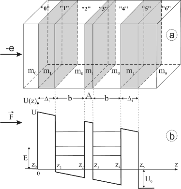
Figure 1: Geometrical (a) and potential energy (b) schemes of RTS.

It is assumed that the monoenergetic ($E$, the energy) electron current ($n$, the concentration) is falling at the RTS from the left side, perpendicularly to its planes. The small difference between lattice constants of RTS layers-wells (the media: $0,2,4,6$) and layers-barriers (the media: $1,3,5$) allows us to study the nanosystem within the framework of the model of effective masses and rectangular potential barriers

$$m(z)={\left\{{{\begin{array}[]{*{20}c}{m_{0}\hfill}\\ {m_{1}\hfill}\\ \end{array}}}\right.}{\rm,}\quad U(z)={\left\{{{\begin{array}[]{*{20}c}{0,\,\,\,\,\,\,\,\text{in reg.}\,\,0,\,2,\,4,\,6,\hfill}\\ {U,\,\,\,\,\,\,\text{in reg.}\,\,1,\,3,\,\,5.\hfill}\\ \end{array}}}\right.}\,\,$$ (1)

The Schrodinger equation for the electron is written as

$$\ri\hbar{\frac{{\partial\Psi(z,t)}}{{\partial\,t}}}=[H_{0}+H(z,t)]\Psi(z,t){\rm,}$$ (2)

where

$$H_{0}=-{\frac{{\hbar^{2}}}{{2}}}{\frac{{\partial}}{{\partial z}}}{\frac{{1}}{{m\left({z}\right)}}}{\frac{{\partial}}{{\partial z}}}+U(z)-\re F\{z[\theta(z)-\theta(z-z_{5})]+z_{5}\theta(z-z_{5})\}{\rm}$$ (3)

– the Hamiltonian of stationary problem (with constant electric field),

$$H(z,t)=-e\epsilon\{z[\theta(z)-\theta(z-z_{5})]+z_{5}\theta(z-z_{5})\}(\re^{\ri\omega t}+\re^{-\ri\omega t})$$ (4)

– the interaction Hamiltonian of electron with the electromagnetic field varying in time ($\omega$, the frequency) and amplitude of electric field intensity ($\epsilon$).

The solution of equation (2.2) in one-mode approximation, assuming the amplitude of high frequency field to be small  [12, 13, 14, 18], according to the perturbation theory, is as follows:

$$\Psi\left({z,t}\right)=\Psi_{0}\left({z}\right)\re^{-\ri\omega_{0}t}+\Psi_{+1}\left({z}\right)\re^{-\ri\left({\omega_{0}+\omega}\right)t}+\Psi_{-1}\left({z}\right)\re^{-\ri\left({\omega_{0}-\omega}\right)t}\,,\qquad\left({\omega_{0}={{E}\mathord{\left/{\vphantom{{E}{\hbar}}}\right.\kern-1.2pt}{\hbar}}}\right).$$ (5)

Here $\Psi_{0}(z)$ function is the solution of stationary Schrodinger equation

$$H_{0}(z)\,\Psi_{0}(z)=E\,\Psi_{0}(z).$$ (6)

Considering that the energy of electronic current in X0Y plane is negligibly small ($k_{||}=0$) it can be written as follows:

$$\Psi_{0}(z) = \Psi^{(0)}_{0}(z)\theta(-z)+\sum\limits_{p=1}^{5}\Psi^{(p)}_{0}(z)[\theta(z-z_{p-1})-\theta(z-z_{p})]+\Psi^{(6)}_{0}(z)\theta(z-z_{5})$$ (7)

$$= \left(\re^{\ri k^{(0)}z}+B^{(0)}\re^{-\ri k^{(0)}z}\right)\theta(-z)+A^{(6)}\re^{\ri k^{(6)}(z-z_{5})}\theta(z-z_{5})$$

$${}+\sum\limits_{p=1}^{5}\left[A^{(p)}\mathrm{Ai}(\xi^{(p)})+B^{(p)}\mathrm{Bi}(\xi^{(p)})\right]\left[\theta(z-z_{p-1})-\theta(z-z_{p})\right],$$

where $\mathrm{Ai}(\xi),\mathrm{Bi}(\xi)$ are the Airy functions and

$$k^{(0)} = \hbar^{-1}\sqrt{\displaystyle 2m_{0}E},\qquad k^{(6)}=\hbar^{-1}\sqrt{\displaystyle 2m_{0}\left(E+\re Fz_{5}\right)},$$

$$\xi^{(1)} = \xi^{(3)}=\xi^{(5)}=\displaystyle\rho^{(1)}\left[(U-E)/\re F-z\right],\qquad\rho^{(1)}=\rho^{(3)}=\rho^{(5)}=\displaystyle(2m_{1}\re F/\hbar^{2})^{1/3},$$

$$\xi^{(2)} = \xi^{(4)}=-\displaystyle\rho^{(2)}\left(E/\re F+z\right),\qquad\rho^{(2)}=\rho^{(4)}=\displaystyle(2m_{0}\re F/\hbar^{2})^{1/3}.$$ (8)

The unknown coefficients ($B^{(0)},A^{(6)},A^{(p)},B^{(p)}\,\ (p=1,\dots,6)$) are fixed by the fitting conditions for the wave functions and their densities of currents at all media interfaces

$$\Psi_{0}^{(p)}(z_{p})=\Psi_{0}^{(p+1)}(z_{p}),\quad\quad\displaystyle\frac{1}{m_{0(1)}}\left.\frac{\rd{\rm\,\ ;}\Psi_{0}^{(p)}}{\rd z}\right|_{z=z_{p}}=\frac{1}{m_{1(0)}}\left.\frac{\rd{\rm\;}\Psi_{0}^{(p+1)}(z)}{\rd z}\right|_{z=z_{p}},\qquad(p=0,\dots,5)$$ (9)

together with the normalizing condition

$$\int\limits_{-\infty}^{\infty}\Psi_{0}^{*}(k^{\prime}z)\Psi_{0}(kz){\rm\;}\rd z=\delta(k-k^{\prime}).$$ (10)

In order to define the both terms of corrections ($\Psi_{\pm 1}(z)$) to wave function, taking into account equations (2.2)–(2.6) and preserving the magnitudes of the first order, inhomogeneous equations are obtained:

$$[H_{0}(z)-\hbar(\omega_{0}-\omega)]\Psi_{\pm 1}(z)-\re\epsilon\{[\theta(z)-\theta(z-z_{5})]+z_{5}\theta(z-z_{5})\}\Psi_{0}(z)=0.$$ (11)

Their solutions are the superposition of functions

$$\Psi_{\pm 1}(z)=\Psi_{\pm}(z)+\Phi_{\pm}(z),$$ (12)

where $\Psi_{\pm}(z)$ are the partial solutions of homogeneous and $\Phi_{\pm}(z)$ are the partial solutions of inhomogeneous equations (2.11).

The solutions of homogeneous equations are

$$\Psi_{\pm}(z) = \Psi^{(0)}_{\pm}(z)\theta(-z)+\sum\limits_{p=1}^{5}\Psi^{(p)}_{\pm}(z)[\theta(z-z_{p-1})-\theta(z-z_{p})]+\Psi^{(6)}_{\pm}(z)\theta(z-z_{5})$$ (13)

$$= B^{(0)}_{\pm}\re^{-\ri k^{(0)}_{\pm}z}\theta(-z)+A^{(6)}_{\pm}\re^{\ri k^{(6)}_{\pm}(z-z_{5})}\theta(z-z_{5})$$

$${}+\sum\limits_{p=1}^{5}\left[A^{(p)}_{\pm}\mathrm{Ai}(\xi^{(p)}_{\pm})+B^{(p)}_{\pm}\mathrm{Bi}(\xi^{(p)}_{\pm})\right]\left[\theta(z-z_{p-1})-\theta(z-z_{p})\right],$$

where

$$k^{(0)}_{\pm} = \hbar^{-1}\sqrt{\displaystyle 2m_{0}(E\pm\hbar\omega)},\qquad k^{(6)}_{\pm}=\hbar^{-1}\sqrt{\displaystyle 2m_{0}\left(E\pm\hbar\omega+\re Fz_{5}\right)},$$

$$\xi^{(1)}_{\pm} = \xi^{(3)}_{\pm}=\xi^{(5)}_{\pm}=\displaystyle\rho^{(1)}\left\{[U-(E\pm\hbar\omega)]/\re F-z\right\},\qquad\xi^{(2)}_{\pm}=\xi^{(4)}_{\pm}=-\displaystyle\rho^{(2)}\left[(E\pm\hbar\omega)/\re F+z\right].$$

The partial solutions of inhomogeneous equations (2.11), as it is shown, are of an exact analytical form

$$\Phi_{\pm}(z)\!\!\! \!=\! \!\displaystyle\pi\frac{\epsilon}{F}\sum\limits_{p=1}^{5}\displaystyle\left[\mathrm{Bi}(\xi^{(p)}_{\pm})\int\limits_{1}^{\xi^{(p)}}\left(\eta-\rho^{(p)}\frac{U(z)-E}{\re F}\right)\mathrm{Ai}\left(\eta\mp\rho^{(p)}\frac{\hbar\omega}{\re F}\right)\Psi_{0}^{(p)}(\eta)\rd\eta\right.$$ (15)

$$\left.{}-\displaystyle\mathrm{Ai}(\xi^{(p)}_{\pm})\!\!\int\limits_{1}^{\xi^{(p)}}\!\!\left(\eta-\rho^{(p)}\frac{U(z)-E}{\re F}\right)\!\mathrm{Bi}\left(\eta\mp\rho^{(p)}\frac{\hbar\omega}{\re F}\right)\Psi_{0}^{(p)}(\eta)\rd\eta\right]\!\![\theta(z-z_{p-1})-\theta(z-z_{p})]$$

$${}\mp\displaystyle\frac{\re\epsilon z_{5}}{\hbar\omega}\Psi_{0}^{(6)}(z_{5})\theta(z-z_{5}).$$

The conditions for $\Psi(z,t)$ wave function continuity (2.5), at all nanosystem interfaces, lead to the boundary conditions for the $\Psi_{\pm 1}(z)$

$$\Psi_{\pm 1}^{(p)}(z_{p})=\Psi_{\pm 1}^{(p+1)}(z_{p}),\qquad\displaystyle\frac{1}{m_{0(1)}}\left.\frac{\rd{\rm\;}\Psi_{\pm 1}^{(p)}}{\rd z}\right|_{z=z_{p}}=\frac{1}{m_{1(0)}}\left.\frac{\rd{\rm\,\ ;}\Psi_{\pm 1}^{(p+1)}(z)}{\rd z}\right|_{z=z_{p}},\qquad(p=0,\dots,5).$$ (16)

The solution of the system of inhomogeneous equations (2.16) defines all unknown coefficients ($B^{(0)}_{\pm}$, $A^{(6)}_{\pm}$, $A^{(p)}_{\pm}$, $B^{(p)}_{\pm}$). Now, $\Psi_{\pm}(z)$ functions (2.13) and $\Psi_{\pm 1}(z)$ corrections (2.15) are definitively written, since $\Psi(z,t)$ being the whole wave function, is fixed too.

Introducing the energy of interaction between the electron and electromagnetic field, which can be calculated as a sum of electronic wave energies flowing from both sides of RTS due to the current, the real part of active conductivity in quasiclassic approximation [19] is determined by densities of currents with the energies

$$\sigma(\omega)=\displaystyle\frac{\hbar\omega}{2z_{5}e\epsilon^{2}}\left\{[j(E+\hbar\omega,z_{5})-j(E-\hbar\omega,z_{5})]-[j(E+\hbar\omega,0)-j(E-\hbar\omega,0)]\right\}.$$ (17)

According to the quantum mechanics, the density of current of uncoupling electrons with concentration $n$ is related to the whole wave function

$$j(z,t)=\displaystyle\frac{\re\hbar n}{2m(z)}\left[\Psi(z,t)\frac{\partial}{\partial z}\Psi^{\ast}(z,t)-\Psi(z,t)\frac{\partial}{\partial z}\Psi(z,t)\right].$$ (18)

Thus, taking into account the expressions (2.5), (2.17) and (2.18), we obtain the final expression for the real part of nanosystem active conductivity

$$\sigma(\omega)=\sigma_{\mathrm{l}}(\omega)+\sigma_{\mathrm{r}}(\omega),$$ (19)

where

$$\sigma_{\mathrm{l}}(\omega)=\displaystyle\frac{\hbar^{2}\omega n}{2z_{5}m_{0}\epsilon^{2}}(k^{(0)}_{+}|B^{(0)}_{+}|^{2}-k^{(0)}_{-}|B^{(0)}_{-}|^{2}),$$ (20)

$$\sigma_{\mathrm{r}}(\omega)=\displaystyle\frac{\hbar^{2}\omega n}{2z_{5}m_{0}\epsilon^{2}}(k^{(6)}_{+}|A^{(6)}_{+}|^{2}-k^{(6)}_{-}|A^{(6)}_{-}|^{2}),$$ (21)

$\sigma_{\mathrm{r}}(\omega),\sigma_{\mathrm{l}}(\omega)$ are the conductivities, stipulated by electronic current interacting with electromagnetic field and flowing out ($\mathrm{r}$ – right side) and back ($\mathrm{l}$ – left side) of nanosystem.

3 Analysis of the results

The numeric calculations and analysis of the symmetric three-barrier RTS conductivity ($\sigma$) and function of the electric field intensity, $F$ (equal to the magnitude of energy shift $U_{0}=\re Fz_{5}$) were performed for In_0.53Ga_0.47As/In_0.52Al_0.48As open nanoheterosystem with physical parameters: $m_{0}=0.089m_{e}$, $m_{1}=0.046m_{e}$, $a_{0}=0.5867$ nm, $a_{1}=0.5868$ nm, $U=516$ meV. The geometrical sizes of wells and barriers were taken in the ranges of values typical of the experimentally investigated nanosystems [1, 2, 3, 4, 5, 6, 7, 8]. It was assumed that the current of monoenergetic electrons with concentration $n=10^{16}$ cm^-3 and energy $E$, corresponding to the resonance energy of the second quasistationary state ($E_{n=2}$), falls at the RTS from the left side.

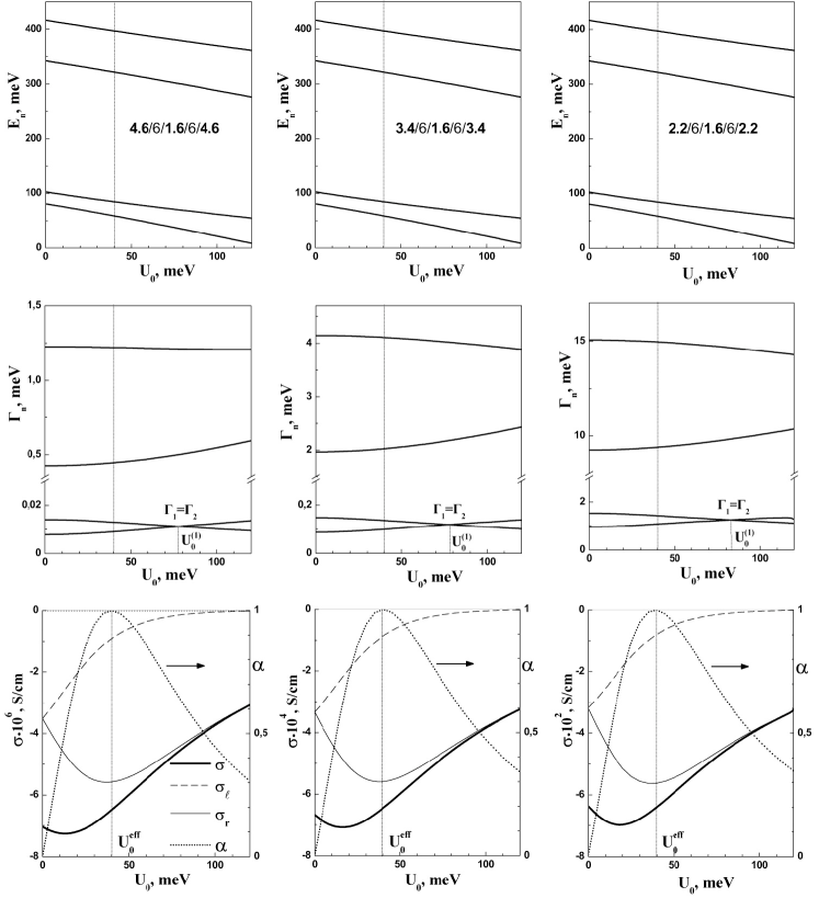
Figure 2: Dependences of resonance energies ($E_{n}$), widths ($\Gamma_{n}$), conductivity ($\sigma$), its terms ($\sigma_{\mathrm{l}},\sigma_{\mathrm{r}}$) and parameter of efficiency ($\alpha$) on energy shift ($U_{0}=\re Fz_{5}$) and three different magnitudes the thicknesses of outer barriers at the fixed sizes of the inner barrier ($\Delta=1.6$ nm) and the widths of wells ($b=6$ nm).

Figure 2 shows the dependences of resonance energies spectrum ($E_{n}$) and resonance widths ($\Gamma_{n}$) of electron quasistationary states and conductivity ($\sigma$) at the transition from the second to the ground quasistationary state and its terms ($\sigma_{\mathrm{r}}$ – due to the right-side current and $\sigma_{\mathrm{l}}$ – due to the left-side current) on the magnitude of electromagnetic field shift ($U_{0}$) at the fixed: $b=6$ nm (wells), $\Delta=1.6$ nm (inner barrier) and $\Delta_{1}=2.2$ nm; 3.4 nm; 4.6 nm (three different magnitudes of outer barriers). In figure 2: In_0.52Al_0.48As barrier layers are in bold, In_0.53Ga_0.47As well layers are in roman. There is also calculated and presented in the same figure an important parameter $\alpha=\sigma(\sigma_{\mathrm{r}}-\sigma_{\mathrm{l}})/\mathrm{max}[\sigma(\sigma_{\mathrm{r}}-\sigma_{\mathrm{l}})]$, characterizing the optimal efficiency RTS acting on condition that for the fixed geometric design of its parts and energy shift ($U_{0}$), both the conductivity ($\sigma$) proportional to the force of laser radiation and the magnitude ($\sigma_{\mathrm{r}}-\sigma_{\mathrm{l}}$) proportional to the current flowing through the RTS would be optimal at the same time.

From figure 2 one can see the following. The magnitudes of resonance energies ($E_{n}$) are almost independent of the thicknesses of outer barriers ($\Delta_{1}$) at the fixed sizes of wells ($b$). At the $U_{0}$ increasing (equal to the increasing intensity of the electric field) all resonance levels show the linear shift into the region of smaller energies. At the same time, the resonance widths ($\Gamma_{n}$) of odd states are increasing and even decreasing. Consequently, there exist such magnitudes of shifts ($U_{0}^{(p)}$), at which the resonance widths of neighbouring states are equal. At the increasing thicknesses of RTS outer barriers, $U_{0}^{(p)}$ magnitudes do not almost vary and resonance widths exponentially increase.

According to the developed theory, the intensity of laser radiation at the frequency $\omega=(E_{2}-E_{1})/\hbar$ would be almost proportional to the maximal magnitude of negative conductivity $\sigma$, arising at the transitions of electrons from the second into the ground quasistationary state. From figure 2 it is clear that $\sigma$ absolute value firstly increases till certain maximum value and further linearly decreases for the bigger $U_{0}$, independently of RTS geometrical parameters. This takes place due to the same $\sigma_{\mathrm{r}}$ bahaviuor while $\sigma_{\mathrm{l}}$ (absolute value) only decreases at $U_{0}$ increasing.

Figure 2 shows that the parameter of optimal effectiveness ($\alpha$) has one maximum at such $U_{0}^{\mathrm{eff}}$ (for the system under research, $U_{0}^{\mathrm{eff}}\approx 40$ meV relating to the electric field intensity $F=18$ kVcm${}^{-1};20$ kVcm${}^{-1};22$ kVcm^-1 for the three different sizes of nanosystem) the magnitude of which almost does not depend on the sizes of outer barriers at the fixed sizes of wells and outer barriers. It is obvious that $U_{0}^{\mathrm{eff}}$ magnitude almost coincides with the shift at which $\sigma_{\mathrm{r}}$ approaches its extremum. Thus, a certain intensity of constant electric field realizing the shift $U_{0}^{\mathrm{eff}}$ at which the nanosystem, as an active element of QCL, works optimally, exists for the fixed geometrical configuration of symmetrical three-barrier RTS.

As far as the increase of the sizes of the outer barriers causes an exponential increase of conductivity, as it is clear from figure 2, when the thicknesses of the outer barriers become bigger than two lattice constats, the conductivity becomes about two orders bigger. Naturally, it does not mean that by increasing the sizes of outer barriers one can obtain the arbitrarily big magnitudes of conductivities because it is obvious that herein the electron lifetime also exponentially increases. For certain sizes of nanosystem, the lifetime becomes much bigger than the relaxation time of electron energy arising due to the electron-phonon, electron-electron and other types of interactions. Therefore, the model which does not take into account these types of energy relaxation becomes useless. Taking this into consideration we studied such sizes of outer barriers at which the electron lifetime in the lowest quasistationary states not bigger than one order exceed the relaxation time due to the interaction with phonons, evaluated in reference [1] approximately as one picosecond.

4 Conclusions

1. For the first time, there is developed a theory of dynamic conductivity of symmetric three-barrier RTS with the exact accounting of the applied constant electric field.

2. It is established that for the fixed geometrical configuration of RTS there exists one minimal magnitude of electric field intensity (equivalent to the energy shift $U_{0}$), at which the active element of QCL works in an optimal regime: the intensity of electromagnetic radiation and density of current flowing through the separate cascade of quantum laser become maximal at the same time.

3. It is shown that within the framework of the used models of effective masses and rectangular potential barriers without taking into account the electron-phonon, electron-electron interactions and other relaxation processes, at the fixed sizes of inner barrier and both wells of three-barrier RTS, the effectiveness of QCL operation exponentially increases both with the increase of outer barriers thicknesses as well with the increases of the magnitude of the shift due to the constant electric field.

Динамiчна провiднiсть симетричної трибар’єрної плоскої наносистеми у постiйному електричному полi Ю.О. Сетi, М.В. Ткач, О.М. Войцехiвська Чернiвецький нацiональний унiверситет iменi Юрiя Федьковича, вул. Коцюбинського, 2,
58012 Чернiвцi, Україна

References

-
[1]
Gmachl C., Capasso F., Sivco D.L., Cho A.Y.,
Rep. Prog. Phys., 2001, 64, 1533;
\bibdoi10.1088/0034-4885/64/11/204. - [2] Scalari G. et al., Appl. Phys. Lett., 2003, 82, 3165; \bibdoi10.1063/1.1571653.
- [3] Diehl L. et al., Appl. Phys. Lett., 2006, 88, 201115; \bibdoi10.1063/1.2203964.
- [4] Qi Jie Wang et al., Appl. Phys. Lett., 2009, 94, 011103; \bibdoi10.1063/1.3062981.
- [5] Hofstetter D., Beck M., Faist J., Appl. Phys. Lett., 2002, 81, 2683; \bibdoi10.1063/1.1512954.
- [6] Gendron L. et al., Appl. Phys. Lett., 2004, 85, 2824; \bibdoi10.1063/1.1781731.
- [7] Giorgetta F.R. et al., Appl. Phys. Lett., 2007, 91, 111115; \bibdoi10.1063/1.2784289.
- [8] Hofstetter D. et al., Appl. Phys. Lett., 2008, 93, 221106; \bibdoi10.1063/1.3036897.
- [9] Elesin V.F., JETP, 2005, 126, 131 (in Russian).
- [10] Elesin V.F., Kateev I.Ju., FTP, 2008, 42, 586 (in Russian).
- [11] Elesin V.F., Kateev I.Ju., Remnev M.A., FTP, 2009, 43, 269 (in Russian).
- [12] Pashkovskii A.B., JETP Lett., 2005, 82, 228 (in Russian).
- [13] Gelvich E.A., Golant E.I., Pashkovskii A.B., JETP Lett., 2006, 32, 13 (in Russian).
- [14] Pashkovskii A.B., JETP Lett., 2009, 89, 32 (in Russian).
- [15] Tkach N.V., Seti Yu.A., Low Temp. Phys., 2009, 35, 556; \bibdoi10.1063/1.3170931.
- [16] Tkach M., Seti Ju., Voitsekhivska O. and Fartushynsky R., AIP Conf. Proc., 2009, 1198, 174; \bibdoi10.1063/1.3284413.
- [17] Tkach M., Seti Ju., Ukr. J. Phys., 2009, 54, 614 (in Ukrainian).
- [18] Golant E.I., Pashkovskii A.B., FTP, 1994, 28, 954 (in Russian).
- [19] Golant E.I., Pashkovskii A.B., Tager A.S., FTP, 28, 740 (in Russian).