The $\Delta$-Statistics of Uncoventional Quarkonium-like Resonances

Abstract

In this note we address the problem of unconventional charmonium-like levels from the standpoint of level spacing theory. The level distribution of the newly discovered vector resonances is compared to that of standard charmonia analyzing their spectral rigidities. It is found that the unconventional charmonium-like states are significantly more compatible with the hypothesis of being levels from a Gaussian Orthogonal Ensamble of Random Matrices than the standard ones, which in turn seem more likely to be Poisson distributed. We discuss the consequences of this result and draw some hints for future investigations.

Introduction. With the very recent observation of the charged resonances $Z(10610)$ and $Z(10650)$ by the Belle collaboration belle , the family of unconventional quarkonium-like states has further grown. Since the discovery of the $X(3872)$, now observed also in LHC experiments, a long list of new narrow resonances has been found. There is a vast consensus that most of them are multiquark structures although a general picture is still missing. Some of these states occur extremely close and some other far from open-charm or beauty thresholds. For the close-to-thresholds ones, several authors agree that the appropriate interpretation is in terms of $S-$wave $D^{(*)}D^{(*)}$ or $B^{(*)}B^{(*)}$ hadron molecules with a very small binding energy (compatible with zero), yet rather stable to be as narrow as the observation shows. Also the prompt production of $X(3872)$ in $p\bar{p}$ collisions at CDF has been observed making at least questionable the chances of a loosely bound molecule interpretation noiben . On the other hand it has been claimed that final state interactions mechanisms could be at the core of the surprising stability of such a molecular object abrat . Similarly the newly discovered states, the $Z(10610)$ and $Z(10650)$, have immediately been interpreted as hadron molecules volo for their mass values happen to be exactly at the threshold values of $BB^{*}$ and $B^{*}B^{*}$ mesons.

Hadron molecules are meant to be extended tetraquark objects (several fermi in size) in which the strong interaction is conveyed by some long range pion exchange or rescattering mechanism. As opposed to this picture one could theorize the existence of compact tetraquark structures which are just new kind of hadrons with four quarks neutralizing the color within the typical range of strong interactions mainoi . In principle, compact tetraquarks are not expected to be formed at the mass values of meson molecules; on the other hand some $Qq\bar{Q}\bar{q}$ bound state could fluctuate into $(Q\bar{q})(\bar{Q}q)$ or $(Q\bar{Q})(\bar{q}q)$ and the discrete levels of the unknown Hamiltonian binding $Qq\bar{Q}\bar{q}$ should, as a result, be coupled to hadron molecule levels.

In this letter we test the assumption that the known $1^{--}$ resonances located at the mass values ${\cal E}=\{3943,4008,4263,4360,4634,4664\}$ MeV – all of them candidates to be exotic hadrons nb – represent the discrete levels of some unknown compact tetraquark Hamiltonian along the same lines as the standard charmonia at ${\cal S}=\{3096~{}(J/\psi),3686~{}(\psi(2S)),3772,4039,4153,4421\}$ MeV are the levels of the $c\bar{c}$ Hamiltonian with the Cornell potential. Resonances in ${\cal E}$ are all produced in $e^{+}e^{-}$ collisions with initial state radiation. Most of the levels of the exotic set ${\cal E}$ happen to be away from open charm threshold and thus represent a good laboratory to explore the possibility that we are observing the spectrum of a complicated multiquark Hamiltonian; for earlier attempts of this kind see vv .

A very much studied conjecture in the field of quantum chaotic systems bohigas84 , states that spectra of quantum Hamiltonian systems whose classical analogs are described by (strongly) chaotic Hamiltonians show locally the same fluctuation properties as predicted by the so called Gaussian Orthogonal Ensemble (GOE) for large dimensional Random Matrices. A portion of the quantum Hamiltonian spectrum is rescaled to spacing one and the levels so obtained turn out to be distributed as the eigenvalues of the GOE Random Matrices in the limit of large dimensions. In this limit indeed the local properties of Random Matrix eigenvalues are extracted, as the Wigner semicircle appears locally flat. As a consequence the probability distribution of the level spacings is expected to follow closely the Wigner law

$$W(s)=\frac{\pi s}{2}\,\exp\Big{(}{-\frac{\pi s^{2}}{4}}\Big{)}$$ (1)

The eigenvalues of GOE matrices following this distribution show the typical level repulsion features studied at length in the context of nuclear resonances.

Naive formulations of tetraquark semiclassical 4-body Hamiltonians are possible, for example relying on one-gluon-exchange models. Most likely all of them express a chaotic classical dynamics. The Hamiltonian describing the $c\bar{c}$ system is, on the other hand, very close to an integrable one. Thus it is expected to have the level clustering features of the Poisson spacing distribution $P(s)=\exp(-s)$, or at least a discrepant behavior with respect to the GOE eigenvalues.

Using the tool of the spectral rigidity also known as the $\Delta-$Statistics developed initially by Dyson and Mehta we study the short sets ${\cal E}$ and ${\cal S}$ in the attempt of confirming or disproving the picture according to which the ${\cal E}$ levels should more markedly match the expected behavior for the GOE ones than standard charmonia, ${\cal S}$, do. We surprisingly find that this is indeed the case although our explorative analysis has its natural limit in the very limited amount of data at hand - the method of $\Delta-$Statistics has been systematically applied for example in the discussion of nuclear resonances level spacing where the data sets contain order of hundreds of levels.

Yet we believe that this result is to be interpreted as an interesting suggestion which leads us to some speculative considerations we are still working on: $i)$ exotic hadrons (for example those in the ${\cal E}$ set) are just like the $c\bar{c}$ ones but with an additional light quark $q\bar{q}$ component; $ii)$ they fall on the levels of some tetraquark Hamiltonian; $iii)$ once a discrete tetraquark level happens to be located within the level width of a molecular level - centered at some meson; threshold - because of the coupling between the two spectra induced by fluctuations like $Qq\bar{Q}\bar{q}\to(Q\bar{q})(\bar{Q}q)\to Qq\bar{Q}\bar{q}$, the molecular level, otherwise very broad, gets metastable because of a Feshbach-like mechanism.

$\Delta$–Statistics. The spectral rigidity (SR) is a measure of the deviation of a level set from uniform spacing: the more regular the set, the smaller the value of the spectral rigidity. Consider a set of $N$ levels $\{E_{i}\}$ rescaled to unit spacing, namely $E_{N}-E_{1}=N-1\equiv 2L$, and centered with respect to the origin ($E_{1}=-L$ and $E_{N}=L$). The sample cumulative function is

$$C(x)\equiv\sum_{E_{i}>0}\Theta\left(x-E_{i}\right)-\sum_{E_{i}<0}\Theta(E_{i}-x)$$

where $\Theta(x)=1$ if $x\geq 0$ and $\Theta(x)=0$ if $x<0$. The spectral rigidity, in its original form due to Dyson and Mehta, is defined as

$$\Delta_{3}\equiv\frac{1}{2L}\min_{A,\,B}\int_{-L}^{L}\left(C(s)-As-B\right)^{2}\mathrm{d}s$$ (2)

following the notations introduced in dysonIV .

The conjecture above means that a sequence of $N$ experimental levels has to be compared with a sequence of $N$ eigenvalues extracted from an ensemble of random matrices with large dimension $D$. Calculations in metha show that in the large $D$ limit the mean of the SR computed with the Poisson distribution is linear in the number of spacings, while that computed with the GOE  eigenvalue distribution grows only logarithmically: it is therefore possible to discriminate between Poisson and GOE levels. This discrimination is more effective as the number of consecutive levels in the studied sequence grows. In practice, the number of levels available is often too low for $\Delta_{3}$ to provide a clear discrimination between Poisson and Gaussian Orthogonal Ensembles. It is therefore useful to consider a different notion of SR in order to reduce the variance. Following Bohigas et al. bohigas82 we set

$$\Delta_{3}(x,y)\equiv\frac{1}{y}\min_{A,\,B}\int_{x}^{x+y}\left(C(s)-As-B\right)^{2}\mathrm{d}s$$ (3)

where $\Delta_{3}(x,y)$ is a generalization of the Dyson-Mehta estimator, recovered as $y=2L$ and $x=-L$. We thus define a new random variable $\Lambda(w,y)$ built on averaging the spectral rigidity of smaller portions of the dataset

$$\Lambda(w,y)\equiv\frac{1}{2L-y+2w}\int_{-L-w}^{L+w-y}\Delta_{3}(x,y)\mathrm{d}x$$ (4)

where $y$ takes continuous values between $0$ and $2L+2w$, which is the number of spacings of the sequence, while $x$ ranges from $-L-w$ to $L+w-y$. We have thus defined a family of statistical variables depending on $y$ and $w$. $\Delta_{3}$ looks at the whole data set whereas $\Delta_{3}(x,y)$ checks a smaller number of levels and $\Lambda(w,y)$ is his average on the data set. The parameter $w$ is introduced in order to minimize possible finite size effects. The original definition of $\Delta_{3}$ is recovered in the limit $w=0\,,\;y\rightarrow 2L$.

Results. The data sets at hand are ${\cal E}=\{3943,4008,4263,4360,4634,4664\}$ MeV, the candidate exotic levels, and the standard charmonia at ${\cal S}=\{3096~{}(J/\psi),3686~{}(\psi(2S)),3772,4039,4153,4421\}$ MeV. ${\cal E}$ contains the masses in MeV of the $1^{--}$ states $G(3900)\,,\;Y(4008)\,,\;Y(4260)\,,\;Y(4360)\,,\;X(4630)$ and $Y(4660)$. ${\cal S}$ contains the masses of the standard $1^{--}$ charmonia, from the $J/\psi$ to the $\psi(4415)$. A third set ${\cal E}^{\prime}=\{3943,4008,4263,4360,4661\}$ MeV is composed by the same resonances of the first set ${\cal E}$, where the $Y(4630)$ and the $Y(4660)$ are taken to coincide with the $Y_{B}(4660)$ state, as proposed in charmed_baryonium . In this study we will neglect the uncertainties on the masses.

In order to choose the parameter $w$ we are introducing, we study the behavior of $\Lambda(w,y)$ on some test series. We choose $w=1$, because smaller values are insensitive to variations of the spacings at the extrema of the series, whereas greater values are useless as they do not add further information.

From now on we will use the notation $\Lambda(1,y)\equiv\Lambda(y)$. As we deal with 5 and 6 level sequences, we generate a large number of $\Lambda(y)$ samples from GOE and Poisson series. The GOE samples are obtained by diagonalizing 30 random GOE matrices $4000\times 4000$ in size, obtaining 24000 series of 5 levels each and 19980 series of 6 levels each; the number of Poisson samples is similar (24000 and 20000). The integral in $\Delta_{3}(x,y)$ is evaluated analytically, whereas the $\Lambda$’s are obtained by a midpoint rectangle approximation. We choose to evaluate $\Lambda(y)$ for integers and half-integers, with $y\in[0.5,7]$ ($\Lambda(0)$ is identically zero). Note that each experimental data set has to be compared with samples of same cardinality.

A comparison between the statistical properties of $\Delta_{3}$ as a function of the number of spacings and our $\Lambda(y)$ is given in Figure 1. There we introduce the ensemble averages $\langle\cdot\rangle_{{}_{\rm P,GOE}}$ where P stands for averaging against the Poisson Ensemble and GOE is for the Random Matrix ensemble. The ensemble average $\langle\Delta_{3}\rangle_{{}_{\rm P,GOE}}$ is computed exactly in metha . The $\langle\Lambda(y)\rangle_{{}_{\rm P,GOE}}$ is computed via the Monte Carlo sampling described above.

The $\langle\Lambda(y)\rangle_{{}_{\rm P,GOE}}$ have respectively the same linear and logarithmic behavior as $\langle\Delta_{3}\rangle_{{}_{\rm P,GOE}}$, apart from the last points where finite-size effects dominate. A clear discrimination between GOE and Poisson sets is reached at $y$ large.

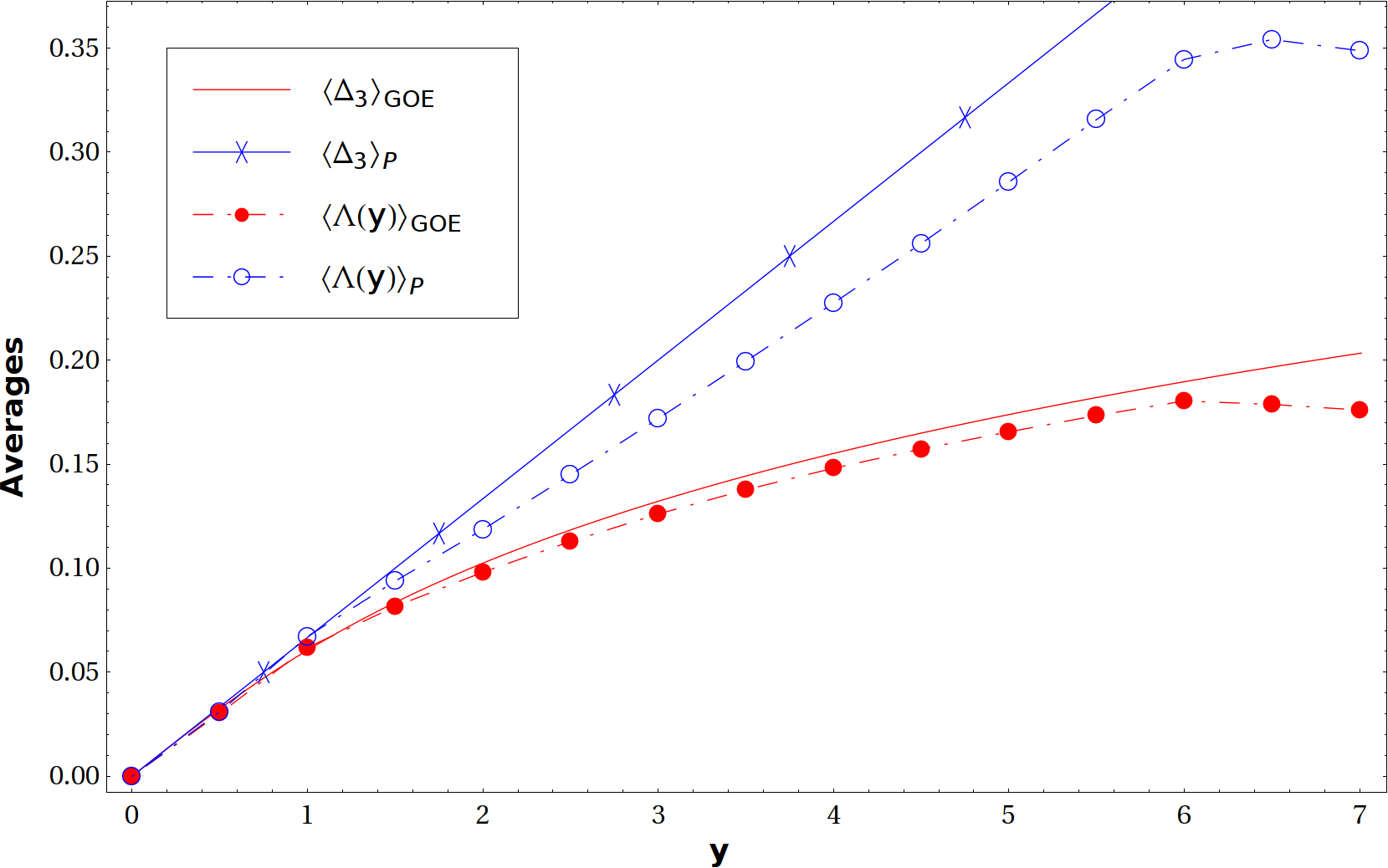
Figure 1: The solid lines represent $\langle\Delta_{3}\rangle_{{}_{\rm P,GOE}}$ for series of $y+1$ levels. The points show the Monte Carlo sampled $\langle\Lambda(y)\rangle_{{}_{\rm P,GOE}}$.

We now study the level properties of the experimental series ${\cal E}$ and ${\cal S}$. We observe that it is hard to discriminate between Poisson and non-Poisson sets because of the large variance of the Poisson $\Lambda(y)$ random variable. On the other hand the GOE distributions have a smaller variance, so a more significant discrimination is possible between GOE and non-GOE sets by looking at high values of $y$.

In Fig. 2 we show the experimental $\Lambda(y)$ for the ${\cal E}$ and ${\cal S}$ levels compared to the six level GOE averages. The results obtained for the sets ${\cal E}$ and ${\cal E^{\prime}}$ are compatible with the hypothesis of GOE distributed levels whereas this turns out not to be true for the ${\cal S}$ set.

Given the random variable $\Lambda(y)$ relative to the GOE ensemble we compute the related distribution function $f_{y}$ as depicted in Fig. 3. We thus introduce

$$\alpha_{y}\equiv\int_{\{s:f_{y}(s)<\bar{f}_{y}\}}f_{y}(s)ds$$ (5)

where $\bar{f}_{y}$ is the value assumed by the distribution $f_{y}$ in correspondence of the SR $\Lambda(y)$ associated to the experimental data set ${\cal S}$. $\alpha_{y}$ takes values in the $[0,1]$ interval; in correspondence of small $\alpha_{y}$ values the null-hypothesis that ${\cal S}$ is a realization of the GOE ensemble has to be rejected.

We consider the most significant five cases $y=5,5.5,6,6.5,7$ and compute the corresponding $\alpha_{y}$ by constructing a binned distribution $f_{y}$. By averaging over different binning choices we obtain the data reported in Table. 1 where for $y\geq 5$ the fraction $\alpha_{y}$ is smaller than 0.1.

$y$	$5$	$5.5$	$6$	$6.5$	$7$
$\alpha_{y}$	$0.097$	$0.084$	$0.095$	$0.096$	$0.089$

Table 1: $\alpha_{y}$ is the fraction of sampled $\Lambda(y)$ whose probability is less than the value $\bar{f}$ introduced in the text.

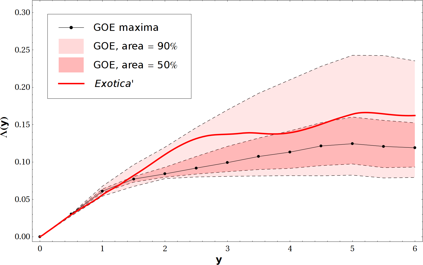
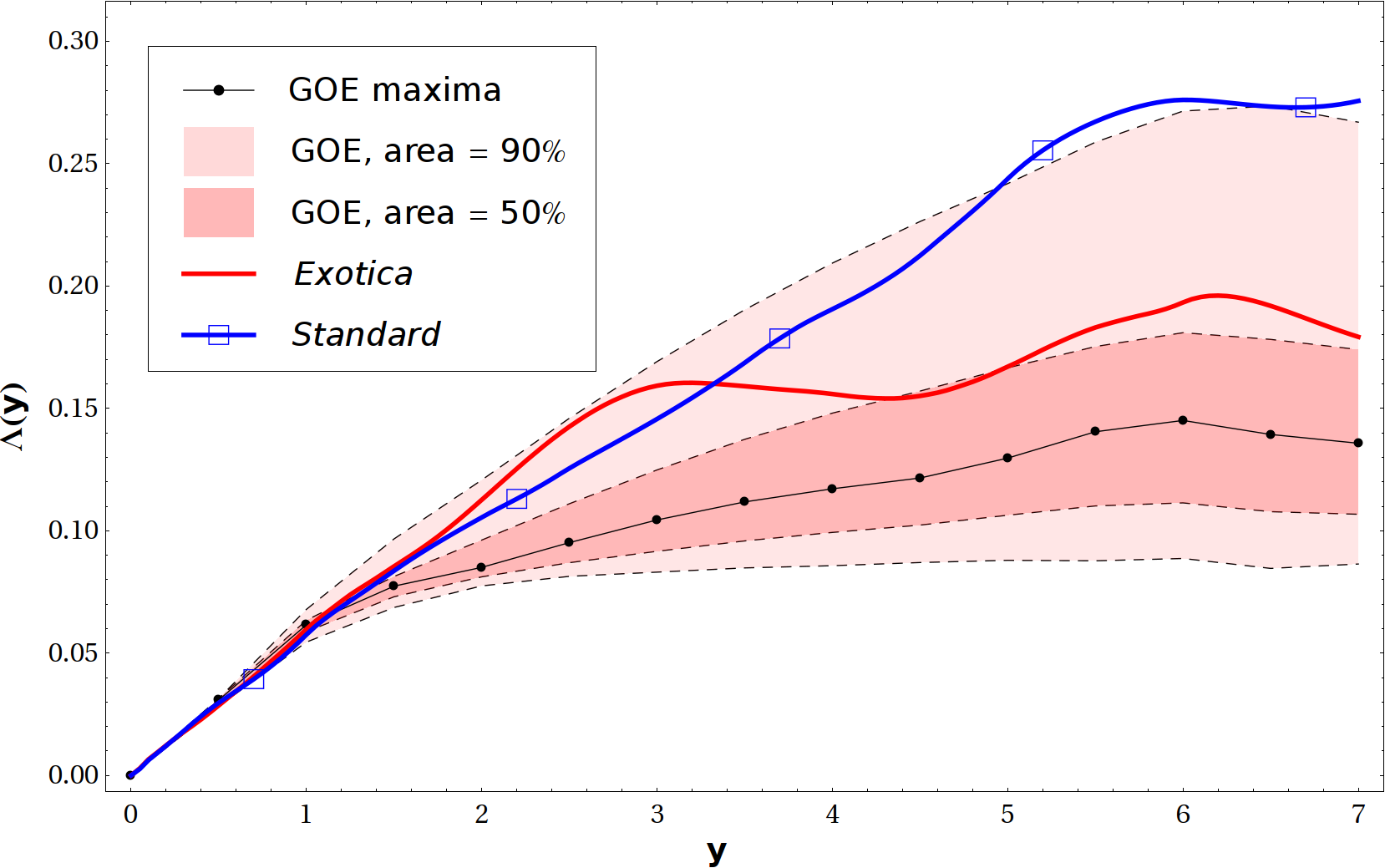
Figure 2: In the two figures the experimental and sampled data for 5-levels (left panel) and 6-levels series are shown. Solid lines show the experimental $\Lambda(y)$ for the $\mathcal{S}$, $\mathcal{E}$ and $\mathcal{E}^{\prime}$ series. For any $y$, the black line indicates the point where the maximum of the distribution $f_{y}$ is attained; the colored areas indicate the regions that contain 50% or 90% of the $\Lambda(y)$ samples. Note that when $\Lambda(y)$ is outside the $90\%$ area, the parameter $\alpha_{y}$ is smaller than $0.1$.

Computing the analogous quantity for the data sets ${\cal E}$ and ${\cal E^{\prime}}$ we get values larger than 0.4 for $y\geq 5$.

It is then reasonable to reject the hypothesis that ${\cal S}$ levels are extracted from the Gaussian Orthogonal Ensemble. Note that, because of the large variance of the Poisson samples, it is practically impossible to reject the hypothesis that a series of few levels ($\lesssim 20$) belongs to the Poisson Ensemble, but, as observed above, it is easier to state that they are not of the GOE type.

As an example in Fig. 3 the sampled distributions for $\Lambda(7)$ are shown and the experimental values of the ${\cal S}$ and ${\cal E}$ sequences.

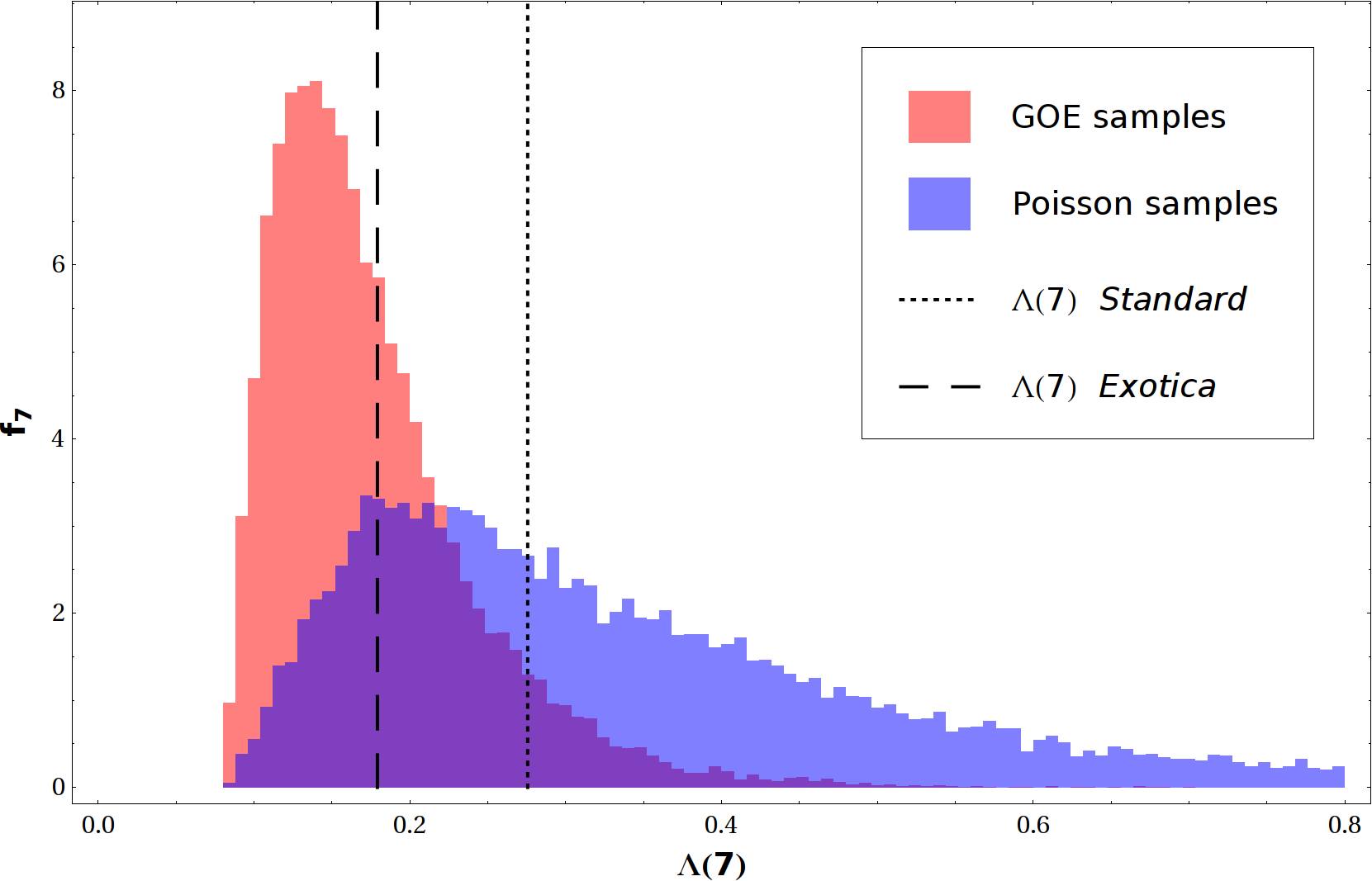
Figure 3: Sampled distributions for $\Lambda(7)$. The histograms are obtained with 19980 GOE samples and 20000 Poisson samples and rescaled to unit area. The vertical lines indicate the $\Lambda(7)$ value for the standard and the exotica series. The bin width is equal 0.008.

Conclusions. Comparing the spectral rigidity of standard $S$-wave charmonia with that of the unconventional vector resonances recently discovered, we observe that the latter states are more significantly compatible with the hypothesis of being the levels of some multiquark Hamiltonian (whose classical analog exhibits chaotic dynamics and therefore having quantum levels distributed with the Wigner law) than the former, which, on the other hand, could be thought as the levels of some classically integrable one - as the simplest version of the Cornell potential Hamiltonian is. The limit of this analysis is in the small amount of experimental data available both in the standard and unconventional sectors. We have introduced a slight modification of the spectral rigidity estimators used in the literature to improve as much as possible the quality of our analysis with a small number of levels.

Molecular Hamiltonians, besides the fact that describe two-body systems, could as well be regulated by complicated potentials with Wigner distributed quantum level spacings. Yet there are states in the ${\cal E}$ sequence of unconventional $1^{--}$ resonances which do not match molecular thresholds whereas the most accredited hadron molecule model has $S$-wave molecules almost exactly at threshold. There are no clear hints on the form of these potentials neither and the main problem of the spectroscopy of the new $X,Y,Z$ resonances remains that of finding a unified description that accounts for both on and off-threshold particles.

Acknowledgements. We wish to thank A. Vulpiani for informative discussions.

References

- (1) Belle Collaboration, arXiv:1105.4583 [hep-ex].
- (2) C. Bignamini, B. Grinstein, F. Piccinini, A. D. Polosa, C. Sabelli, “Is the X(3872) Production Cross Section at Tevatron Compatible with a Hadron Molecule Interpretation?,” Phys. Rev. Lett. 103, 162001 (2009). [arXiv:0906.0882 [hep-ph]].
- (3) P. Artoisenet, E. Braaten, Phys. Rev. D83, 014019 (2011). [arXiv:1007.2868 [hep-ph]].
- (4) A. E. Bondar, A. Garmash, A. I. Milstein, R. Mizuk, M. B. Voloshin, [arXiv:1105.4473 [hep-ph]]; Y. Yang, J. Ping, C. Deng, H. -S. Zong, [arXiv:1105.5935 [hep-ph]]; J. Nieves, M. P. Valderrama, [arXiv:1106.0600 [hep-ph]]; J. Nieves, M. P. Valderrama, [arXiv:1106.0600 [hep-ph]]. A compact tetraquark interpretation is attempted in T. Guo, L. Cao, M. -Z. Zhou, H. Chen, [arXiv:1106.2284 [hep-ph]].
- (5) L. Maiani, F. Piccinini, A. D. Polosa, V. Riquer, “Diquark-antidiquarks with hidden or open charm and the nature of ,” Phys. Rev. D71, 014028 (2005). [hep-ph/0412098].
- (6) N. Brambilla, S. Eidelman, B. K. Heltsley, R. Vogt, G. T. Bodwin, E. Eichten, A. D. Frawley, A. B. Meyer et al., Eur. Phys. J. C71, 1534 (2011). [arXiv:1010.5827 [hep-ph]].
- (7) H. Markum, W. Plessas, R. Pullirsch, B. Sengl, R. F. Wagenbrunn, “Quantum chaos in QCD and hadrons,” [hep-lat/0505011].
- (8) O. Bohigas, M. J. Giannoni, C. Schmit, “Characterization of chaotic quantum spectra and universality of level fluctuation laws,” Phys. Rev. Lett. 52, 1-4 (1984).
- (9) F. Dyson, M. L. Mehta, Statistical Theory of the Energy Levels of Complex Systems. IV. Journal of Mathematical Physics, Volume 4, Number 5, 701, 21 January 1963.
- (10) M. L. Mehta, Random Matrices, Elsevier Academic Press, 3rd Edition, 2004.
- (11) R. U. Haq, A. Pandey, O. Bohigas, “Fluctuations Properties of Nuclear Energy Levels: do Theory and Experiment Agree?”, Phys. Rev. Lett. 48, 1086 (1982).
- (12) G. Cotugno, R. Faccini, A. D. Polosa, C. Sabelli, Phys. Rev. Lett. 104, 132005 (2010). [arXiv:0911.2178 [hep-ph]].