Magnetic anisotropy at nanoscale

Abstract

Nanoscale objects often behave differently than their ‘normal-sized’ counterparts. Sometimes it is enough to be small in just one direction to exhibit unusual features.  One example of such a phenomenon is a very specific in-plane magnetic anisotropy observed sometimes in very thin layers of various materials.  Here we recall a peculiar form of the free energy functional nicely describing the experimental findings but completely irrelevant and thus never observed in larger objects.

1 Intriguing experimental observations

In [1] we find the experimentally observed in-plane magnetic anisotropy energy (MAE) diagrams for multilayer structure Cr$(4)$/Fe$(2)$/Cr$(d_{\mathrm{Cr}})$/Fe$(4)$/Cr$(2)$, where numbers are thicknesses of components, expressed in nm. The thickness of the middle Cr layer, $d_{\mathrm{Cr}}$, was varied in few nm range, and the complete structures were deposited on Si$(100)$ substrate, covered with natural SiO₂ layer $1.5$–$2.0\,$nm thick.  The substrate was not perfectly flat — as a result of ion beam erosion it was covered with quite well ordered ripples (see atomic force microscopy (AFM) images of the substrates, Fig. 1 in [1]). The metallic layers were deposited using molecular beam epitaxy (MBE) technique. Their transmission electron microscopy (TEM) cross sections revealed mostly amorphous structure with small inclusions of polycrystalline character. The values of MAE were derived from hysteresis loop area observed while exciting field was oriented along successive in-plane directions.

In principle, samples of this kind should not exhibit any in-plane magnetic anisotropy. This is indeed the case when the substrate is flat (see Fig. 4a in [1]). On the rippled substrate, however, this is no longer true and the sample exhibits peculiar two-fold in-plane anisotropy (coercive field, Fig. 4b in [1], MAE — in Fig. 4c). It is peculiar since it is not the uniaxial anisotropy: four maxima are visible instead of just two.

2 The surface magnetic anisotropy of a cylinder

Consider the static configuration of individual spins located on a surface of a long (ideally: infinitely long), hollow ferromagnetic cylinder. In absence of any external field one may expect that individual spins may adopt one of the three stable configurations:

• they all may be aligned with $C_{\infty}$ symmetry axis of a cylinder. This is the lowest exchange energy configuration.

• they all may be oriented perpendicularly to the above symmetry axis. Now the exchange energy is no longer at its global minimum. Nevertheless, such a configuration is stable since it realizes a local minimum of exchange energy.

In the second case we may again distinguish two cases: either individual spins are aligned with local $C_{2}$ symmetry axis (there are infinitely many of them, each perpendicular to $C_{\infty}$) thus pointing inwards or outwards of a cylinder and being perpendicular to the cylinder’s surface, or they can be perpendicular to the local $C_{2}$ axis (laying on the cylinder’s circumference), making a ring-shaped configuration, and producing no net magnetization. It is easy to see that both those configurations are energetically equivalent, since the angle between any two neighboring spins is exactly the same.

Here we concentrate only on this part of magnetostatic energy which originates from Heisenberg-type exchange interactions between spins.  For a pair of nearest neighbor ($nn$) spins, say $i$ and $j$, we have

$$E=-2J\,\vec{S}_{i}\cdot\vec{S}_{j}=-2JS^{2}\cos\varphi_{ij},$$ (1)

where $J$ is an exchange integral, $\varphi_{ij}$ is the angle between spins ${i}$ and ${j}$, and $S=\left|\vec{S}_{i}\right|=\left|\vec{S}_{j}\right|$. As the angle $\varphi_{ij}$ between neighboring spins is small, then the following approximation is valid:

$$\cos\varphi_{ij}\approx 1-\varphi_{ij}^{2}/2=1-\frac{1}{2}\left(\frac{\delta}{\rho}\right)^{2},$$ (2)

where $\delta$ is the spacing between $nn$ spins, and $\rho$ is the cylinder radius.

Full magnetostatic energy of a sample is of course the sum, running over all the pairs of $nn$, of expressions like (1). Anisotropy characterizes differences of free energy between various directions of an external field, so any constant terms are meaningless and may be dropped.  In our case such a term is “$1$” in (2).  After this is done, the exchange energy for a single $nn$ pair of spins reads:

$$E\approx J\,\frac{S^{2}\delta^{2}}{\rho^{2}}$$ (3)

As the sum of expressions of type (1) is hard to treat analytically, we replace it with appropriate integral, i.e. we assume the continuous distribution of interacting spins but we do not approximate anything else. Particularly, we do not make use of approximation (2). This way we have to integrate proper expression along the elliptical path, being a trace of a cylinder’s cross-section by a plane parallel to the external magnetic field.  The final result for the surface part of the free magnetostatic energy density, $E_{\mathrm{s}}$, already presented some time ago in [2], reads:

$$E_{\mathrm{s}}=K_{\mathrm{s}}\,\left|\,\cos\theta\,\right|$$ (4)

Here $K_{s}$ is the surface anisotropy constant, and $\theta$ denotes the angle between the direction of sample’s magnetization and easy direction $C_{\infty}$. As one might expect $K_{s}\,\propto\,J/\rho^{2}$ – in full accordance with simplified approach, sketched in (3).

A comment is in order in this place.  Magnetocrystalline anisotropy energy density is always expressed by even powers of $\cos\theta$ and is always a smooth function of the external field orientation.  Here we have $\cos\theta$ in first power, and, additionally, the energy density is not a smooth function.

3 Experimental confirmation

The formula (4) has been first derived to interpret ferromagnetic resonance (FMR) spectrum of Co₆₈Mn₇Si₁₀B₁₅ glass-coated amorphous single microwire with diameter roughly equal to $16.5\,\mu$m.  The spectrum, taken at fixed frequency, and containing more that one absorption line, could not be described (modeled) satisfactorily with conventional two- and fourth-order uniaxial anisotropies alone [3]. Unfortunately, even the inclusion of the surface anisotropy term (4) into the full expression for the free energy density didn’t help much.  This applies also to further experiments, performed on similar but thinner wires, down to the diameter of $6\,\mu$m. Some qualitative features of the spectra (e.g. broadening and distortion of absorption lines at special orientations), however, could be attributed to the presence of a non-smooth surface anisotropy term.  Nevertheless, it had to be concluded that the wire’s diameter was most likely to big to clearly observe the surface anisotropy contribution. By the way, due to the presence of a glassy cover, other effects, notably the magnetostriction of the inhomogeneously stressed sample, were dominating in this experiment.

The definitive confirmation of validity of formula (4) appeared only recently, when the paper [1] was published.  Its authors admit the discrepancy between their model of magnetic anisotropy arising at the interface between two magnetic layers and the experimental data.  Specifically, they expected a quadratic sinusoidal angle dependence but observed additional peaks at $\varphi=90^{\circ}$ and $\varphi=270^{\circ}$, see Fig. 1 in this paper.  Their model mimics quite well the major part of data and curves presented in Fig. 4c [1] but fails to explain the presence of those mysterious ‘additional peaks.’

4 Discussion

Rippled surfaces are well known in experimental practice. Some studies were already performed aiming to gain the full control on ripple formation process on various substrates [4] (sapphire), [5, 6] (silicon), [7] (ZnO), or to investigate the influence of ripples on various physical properties, most notably the magnetic anisotropy, exchange bias [8], or morphology of magnetic domains. Recently many papers are devoted to rippled surfaces of diluted magnetic semiconductors (DMS), with $\mathrm{(Ga,\,Mn)\,As}$ being probably the most frequently studied substance in this class [9, 10].  The active area of research, both theoretical [11, 12] and experimental [13] are competing anisotropies, uniaxial and tetragonal, present in thin layers of this compound.

The rippled surfaces were approximated in literature in many ways, usually as a train of sinusoidal waves, or as a periodic series of Gaussian-shaped peaks or as a periodic set of flat islands.  Here we propose yet another approach, namely the rippled surface may be seen as being build by many identical, infinitely long half-cylinders, aligned parallel to each other.  Obviously, the period of such a structure is equal to $4\rho$, where $\rho$ is, as previously, the individual cylinder’s radius. Additionally, we neglect eventual interactions between cylinders.

We test our theory, given in sec. 2. Using scanned data from Ref. [1], we try to fit them to the expression

$$E(\theta)=a+K_{\mathrm{s}}\,|\cos\theta\,|+K_{\mathrm{u}}\cos^{2}\theta,$$ (5)

i.e. taking into account only the surface anisotropy and conventional uniaxial anisotropy. The constant $a$ is irrelevant, but has to be fitted in order to simulate experimental data correctly. It is therefore not reported in Tab. 1, where the results for two available samples, with different thicknesses $t$, are shown.  The ripple’s period was reported in [1] as being equal to $22\,$nm, so the estimated mean radius of curvature is $5.5\,$nm. This should be compared with the diameter of microwires used in [2].  Looking at the relation (3), it is easy to see why the surface anisotropy term could not be detected in earlier experiments: now the squared radius of curvature is some $3.0\times\,\!10^{5}$—$2.25\times\,\!10^{6}$ times lower, and so many times the expected magnitude of the effect should increase.

Table 1: Fitted parameters of expression (5)

$t$	$\!K_{\mathrm{s}}$	$\!\sigma(K_{\mathrm{s}})$	$\!K_{\mathrm{u}}$	$\!\sigma(K_{\mathrm{u}})$	$\!\left|K_{\mathrm{s}}/K_{\mathrm{u}}\right|$
nm	$\mathrm{kJ/m}^{3}$	$\mathrm{kJ/m}^{3}$	$\mathrm{kJ/m^{3}}$	$\mathrm{kJ/m^{3}}$
$2.0$	$-180$	$6$	$202$	$5$	$0.891$
$5.2$	$-161$	$4$	$184$	$3$	$0.875$

The reported uncertainties for both anisotropy constants, $K_{\mathrm{s}}$ and $K_{\mathrm{u}}$, are most likely seriously underestimated, some $2$—$3$ times, by our quick and dirty fit.  It is quick and dirty because the fitting procedure has no information concerning the uncertainties of individual measurements, and, consequently, treats all the data as being exact.  Even the discretization errors, being a result of manual scanning procedure, go unattended.

Despite of these deficiencies, the trend is clear: the magnitudes of both anisotropy constants slightly decrease with increasing sample’s thickness.

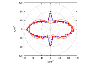
Figure 1: MAE for the sample 2.0 nm thick. In addition to the best fitted line (blue) shown is the ‘pure’ uniaxial part (scaled) of anisotropy. Note the remarkable difference between the two near $\varphi=90^{\circ}$ and $\varphi=270^{\circ}$. $156$ measurements.

The decrease of $K_{\mathrm{s}}$ probably has its roots in decreasing height of ripples, while their period stays unchanged during sample growth, hence the curvature radius $\rho$ effectively increases.  This is probably also the reason for evidently ‘rounded’ shape of peaks visible in Fig. 2.  This feature may be also explained by finite lengths of individual cylinders, their misalignment, or even weak, but long-range, interactions between them. Since it not visible so clearly in Fig. 1, then we should attribute it to broadening of height (and, consequently, of curvature radii) distribution while the sample gets thicker.

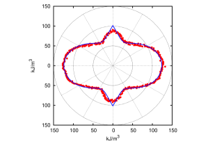
Figure 2: Same as Fig. 1, but for sample $5.2\,$nm thick. $297$ data points. For clarity, the ‘classical’ uniaxial anisotropy term is not shown.

On the other hand, the drop in value of ordinary uniaxial anisotropy $K_{\mathrm{u}}$ originates most likely from the strain relaxation far from possibly mismatched substrate.

It is doubtful whether the presence of sharp, non-differentiable features, existing in reality on any experimental curve will ever be possible to convincingly demonstrate using the data alone. O^′Grady [14] shows, using symmetry arguments, that angular variation of many magnetic properties may be described either as even or as odd series of $\cos\theta$.  Similar ideas, related to variation of coercivity or exchange bias field, were presented even earlier [15]. Here we show one more possibility: the surface anisotropy is described by a single $\left|\,\cos\theta\,\right|$ term, rather hard to approximate by only few terms of even cosine series.

It remains to be explained why $K_{\mathrm{s}}$ in Tab. 1 is expressed in kJ/m³ rather than in kJ/m². This is intended, as it illustrates convincingly (in last column) comparable shares of both types of anisotropy in free energy (not its density!). In fact, what we present there is the quantity $K_{\mathrm{s}}=K^{\prime}_{\mathrm{s}}/t$, where $K^{\prime}_{\mathrm{s}}$ is the true surface anisotropy, expressed in kJ/m², as it should, and $t$ is the sample thickness. Taking this into account, we have $K^{\prime}_{\mathrm{s}}(2.0\;\mathrm{nm})=-0.36\;\mathrm{erg/cm}^{2}$ and $K^{\prime}_{\mathrm{s}}(5.2\;\mathrm{nm})=-0.84\;\mathrm{erg/cm}^{2}$, respectively. One may wonder why the two estimates differ so much. It is less surprising when we compare the samples’ thickness ($2.0$ and $5.2\;$nm) — in both cases smaller than the radii ($5.5\;$nm) of our hypothetical half-cylinders. This means that our cylinders must be far from perfect, they are most likely flattened, what certainly affects their curvature radii, $\rho$. Nevertheless, the values of $K_{\mathrm{s}}$ decrease with sample thickness, as expected. Published values of $\left|K^{\prime}_{\mathrm{s}}\right|$ are scarce, ranging from $0.032\;\mathrm{erg/cm}^{2}$ to as high as $1.17\;\mathrm{erg/cm}^{2}$ for Fe deposited on GaAs [16]. Our result is of the same order of magnitude.

Let us now estimate the exchange energy per single Fe–Fe pair. The density of elementary cells on $(001)$ surface of $\alpha$-Fe is $n=1/a^{2}\approx 1.214\times 10^{19}\mathrm{m}^{-2}$, where $a=2.870\;\AA$ is $\alpha$-Fe lattice constant.  Therefore the exchange energy, $E_{\mathrm{ex}}$, per $a\times{a}$ square element of a surface is $K_{\mathrm{s}}^{\prime}/n$, i.e. $-2.965\times 10^{-23}\;$J for thinner, and $-6.853\times 10^{-23}\;$J for thicker sample.  From formula (3) we get $J=E_{\mathrm{ex}}\left(\frac{\rho}{S\delta}\right)^{2}$, that is $-3.937\times 10^{-21}\;$J and $-9.099\times 10^{-21}\;$J, respectively, when $S=2.22\;$[$\mu_{\mathrm{B}}$] and $\delta=a\sqrt{3}/2\approx{0.215}\;$nm. Those values should still be divided by the number of $nn$ Fe pairs (4) residing in a said $a\times{a}$ surface element.  This is because the nearest neighbor for any given Fe surface atom is the one laying deeper, inside the elementary cell – as pure iron has $bcc$ structure. This fact has been already accounted for by expressing $\delta$ ($nn$ spacing) as an appropriate fraction of the lattice constant. Finally we obtain $J(2.0\;\mathrm{nm})=-0.98\times 10^{-21}\;$J, and $J(5.2\;\mathrm{nm})=-2.28\times 10^{-21}\;$J.  For comparison, Ref. [17] quotes $J=-1.21\;\times\;10^{-21}\;$J for pure $\alpha$-iron. The correspondence is amazingly good, especially that our model completely neglects RKKY-type exchange, certainly present there, and the estimate is made as if the surface was perfectly flat.

5 Conclusions

The surface anisotropy form, presented here, seems to explain the observed features of magnetic anisotropy energy simply formidably. The shape of angular dependence of MAE is reproduced much better than by any other model. The deduced values of $nn$ exchange coupling strength are in good agreement with those obtained independently. Moreover, they are in full accordance with intuitive understanding what makes the surface layer: no more than two crystal planes are involved. Consequently, the surface layer thickness is lower than the size of a unit cell. Yet, such effect can be easily observed only at nanoscale, that is in samples thin enough. Only then its magnitude is comparable with ordinary uniaxial anisotropy (see the last column of Tab. 1).  One may expect that, at least in the case of iron, a $\sim\!\!{500}\;$nm layer is thick enough to effectively mask surface anisotropy effects.

It is amazing that our original, idealized model of non-interacting, infinitely long half-cylinders, works so well. It is likely that the presence of elongated, but finite length structures, present on nominally flat surfaces, even those obtained by MBE technique, is sufficient to generate this form of anisotropy. On the other hand, it is doubtful whether it will ever be used to determine some parameters it depends on. It is because the presented surface anisotropy term is rather sensitive to the fine details of a surface. Those are probably easier to investigate using one of microscopic techniques.  Nevertheless, using its peculiar angular behavior, and treating it as a ‘background’ of known shape, one should be able to determine important material’s parameters with better accuracy than it was possible earlier.

The presence of non-negligible surface anisotropy, generated by surface curvature, in addition to the edge-related effects, will affect the operation of future spintronic devices.

References

- [1] M. Körner, K. Lenz, M.O. Liedke, T. Strache, A. Mücklich, A. Keller, S. Facsko, and J. Fassbender, Interlayer exchange coupling of Fe/Cr/Fe thin films on rippled substrates, Phys. Rev. B, vol. 80, 214401, 2009.
- [2] M.W. Gutowski, R. Żuberek, and A. Zhukov, Novel Surface Anisotropy Term in the FMR Spectra of Amorphous Microwires, J. Magn. Magn. Mat., vol. 272–276, Suppl., pp. E1145–E1146, 2004
- [3] R. Żuberek, M. Gutowski, H. Szymczak, A. Zhukov, and J. Gonzalez, FMR study of amorphous Co68Mn7Si10B15 glass-coated microwires, phys. stat. sol. (a), vol. 196, No. 1, pp. 205, 2003
- [4] Hua Zhou, Yiping Wang, Lan Zhou, Randall L. Headrick, Ahmet S. Özcan, Yiyi Wang, Gözde Özaydin, Karl F. Ludwig Jr., and D. Peter Siddons, Wavelength Tunability of Ion-bombardment Induced Ripples on Sapphire, http://arXiv.org/abs/cond-mat/0608203
- [5] S.A. Mollick and D. Ghose, Formation of ripple pattern on silicon surface by grazing incidence ion beam sputtering, http://arxiv.org/abs/0904.1311
- [6] S. Bhattacharjee, P. Karmakar, A.K. Sinha, and A. Chakrabarti, Projectile’s mass, reactivity and molecular dependence on ion nanostructuring, http://arxiv.org/abs/1008.0958
- [7] S. Bhattacharjee, P. Karmakar, V. Naik, A.K. Sinha, and A. Charkrabarti, Ripple topography on thin ZnO films by grazing and oblique incidence ion sputtering, http://arxiv.org/abs/1102.3309
- [8] M.O. Liedke, B. Liedke, A. Keller, B. Hillebrands, A. Mücklich, S. Facsko, and J. Fassbender, Induced anisotropies in exchange-coupled systems on rippled substrates, Phys. Rev. B, vol. 75, 220407(R), 2007
- [9] K.Y. Wang, A.W. Rushforth, V.A. Grant, R.P. Campion, K.W. Edmonds, C.R. Staddon, C.T. Foxon, B.L. Gallagher, J. Wunderlich and D. A. Williams, Domain imaging and domain wall propagation in thin films with tensile strain, J. Appl. Phys., vol. 101, pp. 106101, 2007
- [10] S. Piano, X. Marti, A.W. Rushforth, K.W. Edmonds, R.P. Campion, O. Caha, T.U. Schülli, V. Hol, and B.L. Gallagher, Surface morphology and magnetic anisotropy in , http://arxiv.org/abs/1010.0112
- [11] A.N. Bogdanov, I.E. Dragunov, U.K. Roessler, Reorientation, multidomain states and domain walls in diluted magnetic semiconductors, J. Magn. Magn. Mat., vol. 316, pp. 225-228, 2007
- [12] A.A. Leonov, U.K. Roessler, A.N. Bogdanov, Phenomenological theory of magnetization reversal in nanosystems with competing anisotropies, http://arxiv.org/abs/0805.1984
- [13] Y.Y. Zhou, X. Liu, and J.K. Furdyna M.A. Scarpulla and O.D. Dubon, Ferromagnetic resonance investigation of magnetic anisotropy in synthesized by ion implantation and pulsed laser melting, Phys. Rev. B, vol. 80, pp. 224403, 2009
- [14] L.E. Fernandez-Outon, K. O’Grady, Angular dependence of coercivity and exchange bias in IrMn/CoFe bilayers, J. Magn. Magn. Mat., vol. 290–291, pp. 536-539, 2005
- [15] T. Ambrose, R.L. Sommer, and C.L. Chien, Angular dependence of exchange coupling in ferromagnet/antiferromagnet bilayers, Phys. Rev. B, vol. 56, pp. 83–86, 1997
- [16] Kh. Zakeri, Th. Kebe, J. Lindner, M. Farle, Magnetic anisotropy of Fe/GaAs(0 0 1) ultrathin films investigated by in situ ferromagnetic resonance, J. Magn. Magn. Mat., vol. 299, pp. L1—L10, 2006
- [17] Richard P. Boardman, Computer simulation studies of magnetic nanostructures, Ph.D. Thesis, Univ. of Southampton, http://www.soton.ac.uk/~rpb/thesis/node18.html 2006-11-28