Spectral decomposition and matrix element effects in scanning tunneling spectroscopy of Bi₂Sr₂CaCu₂O_8+δ.

Abstract

We present a Green’s function based framework for modeling the scanning tunneling spectrum from the normal as well as the superconducting state of complex materials where the nature of the tunneling process$-$ i.e. the effect of the tunneling ’matrix element’, is properly taken into account. The formalism is applied to the case of optimally doped Bi₂Sr₂CaCu₂O_8+δ (Bi2212) high-Tc superconductor using a large tight-binding basis set of electron and hole orbitals. The results show clearly that the spectrum is modified strongly by the effects of the tunneling matrix element and that it is not a simple replica of the local density of states (LDOS) of the Cu-$d_{x^{2}-y^{2}}$ orbitals with other orbitals playing a key role in shaping the spectra. We show how the spectrum can be decomposed usefully in terms of tunneling ’channels’ or paths through which the current flows from various orbitals in the system to the scanning tip. Such an analysis reveals symmetry forbidden and symmetry enhanced paths between the tip and the cuprate layers. Significant contributions arise from not only the CuO₂ layer closest to the tip, but also from the second CuO₂ layer. The spectrum also contains a longer range background reflecting the non-local nature of the underlying Bloch states. In the superconducting state, coherence peaks are found to be dominated by the anomalous components of Green’s function.

I Introduction

High resolution scanning tunneling spectroscopy (STS) together with other highly resolved spectroscopies such as angle resolved photoemission (ARPES), is making it possible to obtain a comprehensive mapping of the electronic spectrum of the high-temperature superconductors (HTSs) in both real and reciprocal space over a wide range of dopings and temperatures. These studies are providing insight into the rich phase diagrams of the HTSs, and are leading thus to an understanding of the ’missing links’ for developing a definitive theory of how high superconducting transition temperatures arise in these unconventional materials. In STS experiments, the focus to date has been on hole doped cuprates, especially on Bi₂Sr₂CaCu₂O_8+δ (Bi2212), which has been the subject of an overwhelming amount of experimental work, see, e.g, Refs. Fischer, ; McElroy, ; Hudson, ; Pan, ; Yazdani, ; Balatsky1, . Bi2212 is a typical cuprate material, which is an antiferromagetic insulator in the strongly underdoped regime, but exhibits a superconducting phase over a wide range of hole doping.

STS can be applied to a substantial part of the doping and temperature spanned phase space of HTS materials. The superconducting (SC) phase is observed around optimal hole doping (OP), while the pseudogap (PG) phase is found within the underdoped regime (UD). As a practical limitation, STS requires a conducting sample, but the deeply underdoped regime is insulating and hence unreachable by STS. However, under experimental conditions the samples are not homogeneously doped. Rather, there is a strong spatial variation in doping, which makes observation of a continuum from the PG to the SC phase possible within one sample. Although these spatial variations in STS generally appear irregular, quite recently a more ordered coexistence of PG and SC phases has been observed Kohsaka .

The physics of the cuprates is dominated by the cuprate layers, which are usually not exposed to the tip of the apparatus. For example, in Bi2212, the quasiparticle tunneling takes place through insulating BiO and SrO layers. The conventional interpretation of the spectra is based on the assumption that the STS spectrum is directly proportional to the LDOS of the CuO₂ layer, especially the LDOS of the $d_{x^{2}-y^{2}}$ orbitals, thus neglecting the effects of the tunneling process in modifying the spectrum in the presence of the insulating overlayers and multiple orbitals. The motivation for this simplification is an attempt to reduce the quasiparticle structure to few band models, which are amenable to theoretical treatment of strong correlation effects in the presence of superconducting and antiferromagnetic order. Notably, there have been attempts to take the effect of the overlayers into account by assuming a ‘tunneling matrix element’ or a ‘filter function’ Balatsky ; hoogenboom ; Fischer .

With this background, our recent work on STSNLMB of Bi2212 provides a significant advance in realistic material-specific modeling of the STS spectrum. We invoke a Green’s function approach where a large number of orbitals is included, and all tunneling paths to the tip in the semi-infinite solid are taken into account. We showed clearly that instead of being a simple reflection of LDOS of the Cu-$d_{x^{2}-y^{2}}$ orbitals, the STS signal represents a very complex mapping of the electronic structure of the system.

In this study we extend our approach by decomposing the tunneling current in terms of regular and anomalous matrix elements of the spectral function in an atomic orbital basis. As in Ref. NLMB, , we concentrate on Bi2212 as the canonical HTS material. We start by reformulating the well-established methods to model tunneling current in nanostructures into a more transparent form for interpreting tunneling in the superconducting state. Our derivation is based on the conventional Todorov-Pendry Todorov ; Pendry approach (TP), which is closely related to the more common Tersoff-Hamann Tersoff method (TH). TP and TH methods both employ a calculation of the LDOS, but TP is more naturally written in terms of Green’s functions. We will show, in fact, that TP decomposes into matrix elements of the spectral function, giving very detailed information concerning the origin of various features in the tunneling spectrum. We thus demonstrate how the contribution of different atomic orbitals to the total current can be extracted from the calculations. Our spectral decomposition also naturally distinguishes between the electron and hole nature of the quasiparticles in the superconducting state. In addition, it leads to a multiband generalization of filtering function by Martin et al Balatsky and a clarification of selection rules governing tunneling through filtering layers. This information is important, e.g., in determining how a dopant or impurity atom alters the spectrum, and how the effect of such a perturbation is seen in real space.

In order to gain a handle on the effects of filtering layers, we derive a consistent form of a filter function through Green’s function manipulations. This rigorous form for the filtering effects is useful for determining the relation between the tunnel current and the LDOS of the CuO₂ layers. We show that this relation is nontrivial in that some channels are ‘first-order forbidden’. Thus our new approach shows that no direct regular signal from $d_{x^{2}-y^{2}}$ orbitals of the Cu directly below the STM tip reaches the microscope. Instead the $d_{x^{2}-y^{2}}$ orbitals of the four neighboring Cu atoms give a major contribution to the tunneling signal. Although we concentrate on pristine systems in the present work, the results have important implications for inhomogeneous situations – e.g., the relationship between the observed features in the spectrum of an impurity atom and the underlying LDOS. This decomposition also allows treatment of the regular and anomalous propagation of quasiparticles in a superconductor, and on this basis we show that the coherence peaks result from the anomalous electron-hole propagation.

The paper is organized as follows. The model for the geometrical structure and the electronic structure is introduced in Sections II.A and B, respectively. The methods to calculate the Green’s function in the normal and the superconducting state are derived in Sections II.B and C, respectively. The Todorov-Pendry equation for the tunneling current is decomposed into regular and anomalous terms to show not only the proper form of the matrix element but also the partial current terms for any chosen orbital in Section II.D. The formalism is applied to discuss STM topographic maps in Section III.A, and the STS spectrum of Bi2212 in Section III.B. The spectrum is then analyzed in terms of tunneling matrix elements and partial currents in Section III.C. Further comments on symmetry analysis are made in Section IV.A., and remarks on electron extraction/injection are made in Section IV.B. Finally, conclusions are drawn and future applications sketched in Section V. Relevant technical details of the form of boson-electron coupling assumed in the tunnel spectra and of the superconducting state calculations are given in the two appendices.

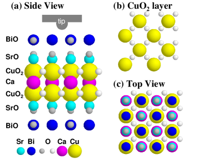
Figure 1: (color online) (a) Side view of the simulation cell used to compute the tunneling spectrum of Bi2212. Tunneling signal from the conducting CuO₂ layers reaches the tip after passing through the filtering layers of SrO and BiO. (b) Cuprate layer showing the supercell consisting of eight primitive cells. (c) Top view of the surface showing the arrangement of various atoms.

II Description of the model

Our theoretical framework involves three distinct steps. First, we choose a three-dimensional geometrical model of atoms with a sufficiently large simulation cell with periodic boundary conditions in the horizontal directions to treat a semi-infinite solid surface. Second, we attach a basis set of atomic orbitals to each atom. At this stage, the one-particle Hamiltonian is constructed and the corresponding Green’s function tensor is formed. Third, we apply our Green’s function formalism to evaluate the tunneling current. The technical details of these three steps are outlined in the following three subsections.

II.1 Sample geometry

We model the Bi2212 sample as a slab of seven layers footnote1 in which the topmost layer is BiO, followed by layers of SrO, CuO₂, Ca, CuO₂, SrO, and BiO, as shown in Fig. 1(a). The tunneling computations are based on a $2\sqrt{2}\times 2\sqrt{2}$ real space supercell consisting of 8 primitive surface cells with a total of 120 atoms (see Fig. 1(b)). The coordinates are taken from the tetragonal crystal structure of Ref. Bellini, . For STS simulations, the STM tip is modeled as an orbital with an s-wave symmetry at the assumed position of the apex of the tip. This tip is allowed to scan across the substrate for generating the topographic maps such as those in Fig. 5, or held fixed on top of a surface Bi atom for the computed spectra presented for example in Fig. 6.

II.2 Construction of the uncorrelated normal state Hamiltonian

In order to construct a realistic framework capable of describing the tunneling spectrum of the normal as well as the superconducting state of the cuprates, we start with the normal state Hamiltonian for the semi-infinite solid in the form

$$\hat{H}_{1}=\sum_{\alpha\beta\sigma}\left[\varepsilon_{\alpha}c^{\dagger}_{\alpha\sigma}c_{\alpha\sigma}+V_{\alpha\beta}c^{\dagger}_{\alpha\sigma}c_{\beta\sigma}\right],$$ (1)

which describes a system of tight-binding orbitals created (or annihilated) via the real-space operators $c^{\dagger}_{\alpha\sigma}$ (or $c_{\alpha\sigma}$). Here $\alpha$ is a composite index denoting both the type of orbital (e.g. Cu-$d_{x^{2}-y^{2}}$) and the site on which this orbital is placed, and $\sigma$ is the spin index. $\varepsilon_{\alpha}$ is the on-site energy of the $\alpha^{th}$ orbital. $\alpha$ and $\beta$ orbitals interact with each other through the potential $V_{\alpha\beta}$ to create the energy eigenstates of the entire system.

The specific electron and hole orbital sets used for various atoms are: ($s,p_{x},p_{y},p_{z}$) for Bi, Ca and O; $s$ for Sr; and ($4s,d_{3z^{2}-r^{2}},d_{xy},d_{xz},d_{yz},d_{x^{2}-y^{2}}$) for Cu atoms. This yields 58 electron or hole orbitals in a primitive cell and a total of $2\times 464$ orbitals in the $2\sqrt{2}\times 2\sqrt{2}$ simulation supercell. The number of k-points used in the computations depends on whether we do band calculations or solve the Green’s function. For band calculations, we use a dense set of k-values to produce smooth bands for directions $\Gamma\rightarrow M\rightarrow X\rightarrow\Gamma$ as seen for example in Fig. 2. In the case of Green’s function calculations, we use $N_{k}=256$ k-points for the supercell Brillouin zone. This corresponds to $8\times 256=2048$ k-points for a primitive cell.

$v_{\alpha\beta m}(eV)$
$v_{ss\sigma}$	$v_{sp\sigma}$	$v_{pp\sigma}$	$v_{pp\pi}$	$v_{sd\sigma}$	$v_{pd\sigma}$	$v_{pd\pi}$	$v_{dd\sigma}$	$v_{dd\pi}$	$v_{dd\delta}$
-0.28	0.94	1.23	-0.13	-0.62	-2.81	1.16	-9.00	12.60	-2.29

$\varepsilon_{\alpha}(eV)$
s/Bi	p/Bi	s/O(Bi)	p/O(Bi)	s/Sr	s/Ca	p/Ca
-12.200	1.800	14.700	-2.400	7.819	5.631	13.335a
s/O(Sr)	p/O(Sr)	s/Cu	d/Cu	s/O(Cu)	p/O(Cu)
-15.270	-2.353	5.001	-2.962	-18.560	-3.825

Table 1: Slater-Koster prefactors, $v_{\alpha\beta m},$ and onsite energies $\varepsilon_{\alpha}.$ The $v_{\alpha\beta m}$ are used to construct the Hamiltonian overlap matrix elements $V_{\alpha\beta}$ as described in Ref. Slater .

The Slater-Koster formalism Slater ; Harrison ; Shi is used to fix the angular dependence of the tight binding overlap integrals. The onsite energies and the prefactors are fitted to the LDA band structure of Bi2212 that underlies for example the extensive angle-resolved photointensity computations of Refs.  bansil99, ; lindroos02, ; bansil05, ; markiewicz05, ; asensio03, ; bansil98, . In Table I, we show the specific values of the $v_{\alpha\beta m}$ prefactors used for computing the Slater-Koster hopping integrals. Notably, we have shifted the bottom of the BiO conduction band to agree with experiments, which do not observe the Bi-bands at least within $1eV$ above the Fermi-level. This choice is also supported by calculations of Ref. HL, , which show the sensitivity of the position of the Bi-band with respect to impurities and doping. The absence of the bottom of the BiO band in the STS spectra may also be due to a voltage gradient across the insulating filter layers (BiO and SrO layers) when applying a bias voltage between the tip and the sample. If so, the absolute value of the voltage within these layers is less than the bias voltage $V_{b}$, and thus the apparatus would need to apply a bias which would be significantly larger than $V_{b}$ to locally see states that are strictly at $E_{F}+eV_{b}.$

The tight-binding parameters of the normal state Hamiltonian of Eq. (1) produce the detailed band structure of Bi2212 shown in Fig. 2. While the tight-binding band structure is in reasonable agreement with the LDA band structure of Ref. HL, , in order to carry out spectroscopic computations, one must additionally make sure that the underlying wavefunctions are described correctly including their symmetries. Our procedure based on the the use of Koster-Slater matrix elements not only fits the band stuctures, but the symmetries and phases of the associated wavefunctions are also described correctly.

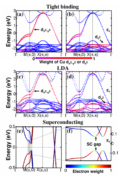
Figure 2: (color online) (a)-(d): Normal state band structure of Bi2212 for the tight-binding Hamiltonian and from first-principles LDA computations. Weights of Cu-$d_{x^{2}-y^{2}}$ and Cu-$d_{z^{2}}$ contribution to the bands are shown using a colorscale where red denotes high and blue low values (see colorbar). Note that the tight-binding calculations are done for a slab, so that the the tight-binding bands do not display the splitting of Bi-O bands seen in LDA results. The LDA bands have been calculated using Virtual Crystal Approximation (VCA) with 24% Pb doping to set the bottom of the BiO band. (e) and (f): Quasiparticle band structure in the superconducting state based on the Hamiltonian of Eq. (3) is shown in (e). Panel (f) zooms in on the gap region of (e) which is shaded grey. Electron character of quasiparticles is shown in red and the hole character in blue. Notice, that the quasiparticles differ significantly from being electrons or holes only in the close neighborhood of the superconducting gap around the M-point.

Figs. 2 (a)-(b) show the normal state tight-binding band structure based on our $58$ orbital Hamiltonian of Eq. (1). The main cuprate bands, with predominantly Cu-$d_{x^{2}-y^{2}}$ character, are seen in panels (a) and (b) to follow the corresponding LDA calculations in panels (c) and (d). Note that in our tight-binding modeling, we have adjusted the positions and bilayer splitting of the two van Hove singularities (VHSs) to approximately match the experimental photoemission and STS findings for the optimal doping (OP) region with hole concentration $p\approx 0.16$ (Ref. Gomes, ; Kaminski, ). In addition to Cu-$d_{x^{2}-y^{2}}$, Cu-$d_{z^{2}}$ is seen in panels (b) and (d) to give a significant spectral weight to this band, especially at energies below the Fermi-level. The complicated ‘spaghetti’ region has large contributions from the $d_{z^{2}}$ of Cu and horizontal $p_{x}(p_{y})$ orbitals of the oxygens within the cuprate layer as well as the vertical $p_{z}$ orbital of the apical oxygen. Concerning the filter layers, the bottom of the BiO-like conduction band (or bismuth pocket) along the $M(\pi,0)$ direction carries the character of the horizontal p-orbitals of the surface oxygens $O(Bi)$ (see Fig.  2 (a)).

In tunneling calculations, we directly evaluate the Green’s function instead of diagonalizing the Hamiltonian. For this purpose, the normal state Green’s function is solved first by starting from the orbital matrix elements of the Green’s function:

$$g^{\pm}_{\alpha\beta}=\frac{\delta_{\alpha\beta}}{\varepsilon-\varepsilon_{\alpha}-\Sigma^{\pm}_{\alpha}(\varepsilon)},$$ (2)

where $\varepsilon_{\alpha}$ is the onsite energy of the orbital $\alpha.$ At this point, a diagonal self-energy $\Sigma^{\pm}_{\alpha}=\Sigma_{\alpha}{{}^{\prime}}\pm i\Sigma_{\alpha}{{}^{\prime\prime}}$ can be included straightforwardly. The simplest self-energy is a constant broadening of the states in the form of a convergence factor $\Sigma^{\pm}_{\alpha}=\mp i\eta.$ Appendix A (Eq. (19)) presents a more general self-energy which we use to model electron-boson coupling.

The total Green’s function $G$ is constructed by solving Dyson’s equation

$$G=g+gVG,$$

where $V_{\alpha\beta}$ are the off-diagonal overlap integrals of Eq. (1) Dyson’s equation is exactly solved using the method described in Ref. Nieminen , which is suitable for tunneling calculations footfourier .

II.3 Pairing interaction and the superconducting state Hamiltonian

Superconductivity is included by adding a pairing interaction term $\Delta$ in the Hamiltonian of Eq. (1) as follows

$$\hat{H}=\hat{H}_{1}+\sum_{\alpha\beta\sigma}\left[\Delta_{\alpha\beta}c^{\dagger}_{\alpha\sigma}c^{\dagger}_{\beta-\sigma}+\Delta_{\beta\alpha}^{\dagger}c_{\beta-\sigma}c_{\alpha\sigma}\right]$$ (3)

A gap parameter value of $|\Delta|=0.045eV$ is chosen to model a typical experimental spectrumMcElroy for the illustrative purposes of this study. We take $\Delta$ to be non-zero only between $d_{x^{2}-y^{2}}$ orbitals of the nearest neighbor Cu atoms, and to possess a d-wave form, i.e., $\Delta_{d(d\pm x)}=+|\Delta|$ and $\Delta_{d(d\pm y)}=-|\Delta|,$ where $d$ denotes the $d_{x^{2}-y^{2}}$ orbital at a chosen site, and $d\pm x/y$ the $d_{x^{2}-y^{2}}$ orbital of the neighboring Cu atom in x/y-direction. In momentum space, the corresponding $\Delta$ is given by

$$\Delta_{k}=\frac{\Delta}{2}\left[\cos{k_{x}a}-\cos{k_{y}a}\right],$$ (4)

where $a$ is the in-plane lattice constant. The pairing interaction of Eq. (3) allows electrons of opposite spins to combine to produce superconducting pairs such that the resulting superconducting gap is zero along the nodal directions $k_{x}=\pm k_{y}$, and is maximum along the antinodal directions. This choice of pairing interaction follows, e.g., the one-band formalism given in Ref. Flatte, .

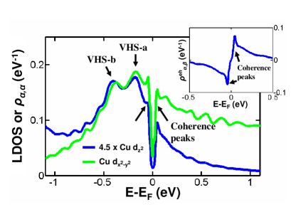
Figure 3: (color online) Main: LDOS (or the diagonal elements $\rho_{\alpha\alpha}$ of the density matrix; see Appendix B for details) of $d_{x^{2}-y^{2}}$ (green) and $d_{z^{2}}$ (blue) orbitals of Cu. [Note $d_{z^{2}}$ curve is scaled up by a factor of 4.5 to compare the shapes of the two LDOSs.] Oscillations at high positive or negative energies ( above $\pm 0.5$ eV) are artifacts due to the use of a sparse mesh of k-points in the computation. Inset: Anomalous density matrix term $\rho^{eh}_{\alpha\beta}$ discussed in Appendix B, where $\alpha$ and $\beta$ denote $d_{x^{2}-y^{2}}$ orbitals of two neighboring Cu atoms.

For treating the superconducting case, we employ the tensor (Nambu-Gorkov) Green’s function ${\cal G}$ (see Ref. Fetter, ) with the corresponding Dyson’s equation:

$${\cal G}={\cal G}^{0}+{\cal GVG}^{0},$$ (5)

where

$${\cal G}=\left(\begin{array}[]{cc}G_{e}&F\\ F^{\dagger}&G_{h}\end{array}\right)~{}\textrm{and}~{}{\cal V}=\left(\begin{array}[]{cc}0&\Delta\\ \Delta^{\dagger}&0\end{array}\right)$$

where $G_{e}$ and $G_{h},$ denote the Green’s functions for the electrons and holes, respectively.

The normal state electron Green function $G_{e}$ can be used to derive the hole Green function $G_{h}$. It can be shown by, e.g., the equation of motion method, that

$$G^{\pm}_{h,\alpha\beta}(E)=-G^{\mp}_{e,\beta\alpha}(-E)$$

It is straightforwardly shown then that

$$G_{e} = G_{e}^{0}+F\Delta^{\dagger}G_{e}^{0}$$

$$F = G_{e}\Delta G_{h}^{0}$$ (6)

The quasiparticle Green’s function projected onto electron degrees of freedom is then written in the form

$$G_{e}=G_{e}^{0}+G_{e}\Sigma^{BCS}G_{e}^{0},~{}\textrm{where}~{}\Sigma^{BCS}=\Delta G_{h}^{0}\Delta^{\dagger}.$$ (7)

We also need the self-energy term $\Sigma^{h}_{\alpha}$ for holes. Since the transformation from electron to holes follows that of the Green’s function, we obtain the general form

$$\Sigma^{h}_{\alpha}(\varepsilon)=-\Sigma^{e*}_{\alpha}(-\varepsilon)=-\Sigma^{{}^{\prime}}_{\alpha}(-\varepsilon)+i\Sigma^{{}^{\prime\prime}}_{\alpha}(-\varepsilon).$$

In our particular case, we use a self-energy with an odd real part and an even imaginary part as discussed in Appendix A (see Eq. (19)) Our self-energy is thus invariant under electron-hole transformation.

Figs. 2(e) and (f) show the modifications of the normal state band structure from the introduction of the pairing interaction. Only the region within $\pm 500meV$ of the Fermi level is shown in panel (e), as the remainder of the bands are unchanged from the normal state results of panels (a) and (b). The superconducting state dispersion in panels (e) and (f) clearly displays a d-wave gap with a maximum in the antinodal region near the $M$ point and zero gap along the nodal direction near $(\pi/2,\pi/2)$. Note that both bonding and antibonding VHSs possess gaps of similar magnitude. Fig. 2(e) also shows the relative electron/hole character of the quasiparticles. As expected, the quasiparticles are very distinctly either electron- or hole-like almost everywhere except within a very narrow energy range at the top and bottom of the SC gap. Fig. 3 further shows that mixing of the electron and hole features gives rise to coherence peaks in the LDOS of Cu-$d_{x^{2}-y^{2}}$ and to a lesser extent in the LDOS of Cu-$d_{z^{2}}$. The effects of electron-hole mixing are however most pronouned in the anomalous matrix element of the quasiparticle Green’s function (inset to Fig. 3 and Fig. 4). In fact, the off-diagonal matrix element between an up-spin $d_{x^{2}-y^{2}}$ electron orbital and a down-spin $d_{x^{2}-y^{2}}$ hole orbital of two neighboring Cu atoms gives the most important term in the anomalous part of the Green’s function. This term has d-wave symmetry, which manifests itself as a change in sign each time we make a rotation of $\frac{\pi}{2}$ around the central Cu site. In addition to the coherence peaks, the anomalous density matrix inherits features from the VHSs in the regular part of the density matrix, which in view of electron-hole symmetry are reflected on both sides of the Fermi energy. Additionally, strong hybridization between up-spin Cu-$d_{x^{2}-y^{2}}$ electron orbitals and down-spin orbitals of O $p_{x}$ holes (and vice versa) takes place as shown in Fig. 4. This term is comparable in strength to the Cu-$d~{}-~{}$Cu-$d$ terms and changes sign in rotations of $\pi$ for reasons explained in the special case (3) of the following paragraph. Fig. 4 also shows a small onsite contribution from the up-spin electron and down-spin hole of the $p_{x}$-orbital on the oxygen between two neighboring Cu atoms. It is notable that these matrix elements strictly follow the d-wave symmetry in rotations around the central Cu atom.

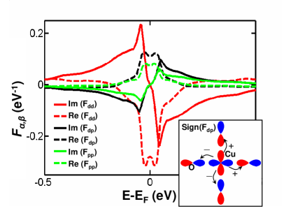
Figure 4: (color online) Main: Matrix elements of the anomalous Green’s function for onsite $p_{x}$-orbital of an intermediate oxygen atom (green lines), $d_{x^{2}-y^{2}}$ orbitals of two neighboring Cu atoms (red lines), and between Cu-$d_{x^{2}-y^{2}}$ and a $p_{x}$ orbital of a neighboring oxygen (black lines). Inset: The directional dependence of the sign of the off-diagonal element $F_{dp}$. For details see special case (3) in the text.

These transformation properties follow consistently from Eq. (6). Let us, for example, look at the equation in the $x$-direction: $F_{\alpha\beta}=G_{e,\alpha d}\Delta_{d(d\pm x)}G^{0}_{h,(d\pm x)\beta},$ where $d$ is a shorthand notation for $d_{x^{2}-y^{2}}$ of a chosen Cu atom, and $d\pm x$ stands for the $d_{x^{2}-y^{2}}$ orbital of the neighboring Cu atom in the positive/negative x-direction and consider several specific cases as follows.
(1) For $\alpha=d$ and $\beta=d\pm x$, both $G_{e,\alpha d}$ and $G^{0}_{h,(d\pm x)\beta}$ are onsite matrix elements, and thus their sign remains invariant when changing from one Cu to another. Hence the term $\Delta_{d(d\pm x)}$ is decisive, and the sign can change only in going from x- to y- direction;
(2) For $\alpha=\beta=$ O-$p_{x},$ we have to first look at the term $G_{e,p_{x}d}G^{0}_{h,(d\pm x)p_{x}}$. Since the relative phases of the off-diagonal matrix elements of the Green’s function are proportional to the sign of the overlap of the two orbitals, it is straightforward to see from the signs of the lobes of the $d$ and $p$ orbitals that this product is invariant to change in direction as well as in going from x to y. Therefore, $\Delta_{d(d\pm x)}$ again gives the d-wave symmetry of these terms;
(3) For $\alpha=d$ and $\beta=$ O-$p_{x}$, $G_{e,\alpha d}$ is diagonal and thus invariant. Considering the overlaps, one sees that

$$G^{0}_{h,(d-x)\beta}=-G^{0}_{h,(d+x)\beta},$$

and

$$G^{0}_{h,(d+y)\beta}=-G^{0}_{h,(d-y)\beta}=-G^{0}_{h,(d+x)\beta}.$$

But, since $\Delta_{d(d\pm x)}=-\Delta_{d(d\pm y)}$,

$$F_{dp_{x}(-)}=-F_{dp_{x}(+)}=-F_{dp_{y}(+)}=F_{dp_{y}(-)},$$

as shown in the inset to Fig. 4.

Eq. (25) of Appendix B shows that $F_{\alpha\beta}\propto\langle c_{\alpha\uparrow}c_{\beta\downarrow}\rangle.$ Hence, case (3) of the last paragraph indicates that there is a significant pairing $\langle c_{d_{x^{2}-y^{2}}\uparrow}c_{\phi\downarrow}\rangle$ when

$$|\phi\rangle\propto|p_{x}(+)\rangle+|p_{y}(+)\rangle-|p_{x}(-)\rangle-|p_{y}(-)\rangle.$$

Recall that we introduced superconductivity in Hamiltonian of Eq. (3) only on the Cu-$d_{x^{2}-y^{2}}$ orbitals. Thus we see that within our model the strong Cu-O hybridization automatically induces pairing on the oxygen orbitals. This pairing is analogous to the concept of Zhang-Rice singlets (ZRS) in the low doping limit Zhang , where pair states

$$|d_{x^{2}-y^{2}}\uparrow\rangle|\phi\downarrow\rangle-|d_{x^{2}-y^{2}}\downarrow\rangle|\phi\uparrow\rangle$$

are formed. Note, however, that ZRS is a concept related to doping levels in the ‘normal’ phase, and is not directly concerned with superconductivity. Nevertheless, the preceding considerations indicate that our model is in accord with the ZRS scenario of the normal state onsitep .

II.4 Green’s function formulation of tunneling current

We turn now to consider the formulation of the tunneling spectrum. For this purpose, we apply the conventional form of the Todorov-Pendry expression Todorov ; Pendry for the differential conductance $\sigma$ between orbitals of the tip ($t,t^{\prime}$) and the sample ($s,s^{\prime}$), which in our case is straightforwardly shown to yield

$$\sigma=\frac{dI}{dV}=\frac{2\pi e^{2}}{\hbar}\sum_{tt^{\prime}ss^{\prime}}\rho_{tt^{\prime}}(E_{F})V_{t^{\prime}s}\rho_{ss^{\prime}}(E_{F}+eV)V_{s^{\prime}t}^{\dagger},$$ (8)

where the density matrix

$$\rho_{ss^{\prime}}=-\frac{1}{\pi}Im[G_{ss^{\prime}}^{+}]=\frac{1}{2\pi i}\left(G^{-}_{ss^{\prime}}-G^{+}_{ss^{\prime}}\right),$$ (9)

is given in terms of the retarded electron Green function or propagator $G_{ss^{\prime}}^{+}$. Eq. (8) differs from the more commonly used Tersoff-Hamann approachTersoff in that it takes into account the details of the symmetry of the tip orbitals and how these orbitals overlap with the surface orbitals.

Since electrons are not eigenparticles in the presence of the pairing term, Dyson’s equation needs to be applied to the Green’s function tensor:

$${\cal G}^{-}={\cal G}^{+}+{\cal G}^{+}({\mathbf{\Sigma}^{-}}-{\mathbf{\Sigma}^{+}}){\cal G}^{-}={\cal G}^{+}-2i{\cal G}^{+}{\mathbf{\Sigma}^{{}^{\prime\prime}}}{\cal G}^{-}$$ (10)

After extracting the electron part from Eq. (10) and applying Eq. (9), the spectral function can be written as:

$$\rho_{ss^{\prime}}=-\frac{1}{\pi}\sum_{\alpha}(G_{s\alpha}^{+}\Sigma{{}^{\prime\prime}}_{\alpha}G_{\alpha s^{\prime}}^{-}+F_{s\alpha}^{+}\Sigma{{}^{\prime\prime}}_{\alpha}F_{\alpha s^{\prime}}^{-}),$$ (11)

Using Eq. (11), the tunneling current of Eq. (8) can be recast into the form

$$\sigma=\sum_{t\alpha}T_{t\alpha},$$ (12)

where

$$T_{t\alpha}=-\frac{2e^{2}}{\hbar}\sum_{t^{\prime}ss^{\prime}}\rho_{tt^{\prime}}(E_{F})V_{t^{\prime}s}(G^{+}_{s\alpha}\Sigma{{}^{\prime\prime}}_{\alpha}G^{-}_{\alpha s^{\prime}}+F^{+}_{s\alpha}\Sigma{{}^{\prime\prime}}_{\alpha}F^{-}_{\alpha s^{\prime}})V_{s^{\prime}t}^{\dagger},$$ (13)

and the Green’s function and the self-energy are evaluated at energy $E=E_{F}+eV_{b}.$ Eqs. (12) and (13) are an extension of the Landauer-Büttiker formula for tunneling across nanostructures (see, e.g., Ref. Meir, ), and represent a reformulation of Refs.  Fisher, and Frederiksen, . By comparing Eqs. (11) and (13), we see that if the tip makes contact with only a single surface atom orbital, e.g., a Bi-$p_{z}$ orbital, then the tunneling current is directly proportional to the LDOS of that orbital. In particular, the tunneling current bears in general no such simple relationship to the quantity of most interest, namely, the LDOS on the CuO₂ plane. Obviously, the tunneling formalism of Eq. (13) must be further elaborated in order to find the relation between the interesting LDOSs and the tunneling spectrum.

II.4.1 Tunneling channels, filter function and tunneling matrix element

The experimental STM spectra in the cuprates have to date been mostly compared to the electronic LDOS of the superconducting cuprate layer, especially the LDOS of the Cu-$d_{x^{2}-y^{2}}$ orbital. The discrepancies between the spectra and the LDOS are then ascribed to ‘tunneling matrix elements’ or ‘filtering functions’ Balatsky . The former refers to the general problem of modeling spectroscopies, where the signal is distorted by the spectroscopic process, and may even vanish due to the presence of selection rules. The latter term refers to how the states of electrons (or quasiparticles) from the initial state within the superconducting layers are modified when traveling through the oxide overlayers before reaching the tip. Eq. (13) above accounts fully for the tunneling process, and it can be reformulated to reveal, for example, the filtering effect more clearly. For this purpose, it is convenient to the denote various orbitals as follows: $s$ and $s^{\prime}$ for the orbitals of the sample surface, which overlap with the tip orbital $t$; $f$ and $f^{\prime}$ for the orbitals of the filter layers, BiO and SrO; $c$ and $c^{\prime}$ for orbitals in the cuprate layer; and, $\alpha$ for any orbital that is singled out, which in our case usually will be an orbital in the cuprate layer. Denoting the Green’s function for the filter layers decoupled from the rest of the system by $G^{0+}_{sf}$, and the matrix elements within the cuprate layer in the coupled system by $G^{+}_{c\alpha}$, application of Dyson’s equation to $G^{+}_{s\alpha}$ yields

$$G^{+}_{s\alpha}=G^{0+}_{sf}V_{fc}G^{+}_{c\alpha}~{}~{}\textrm{and}~{}~{}F^{+}_{s\alpha}=G^{0+}_{sf}V_{fc}F^{+}_{c\alpha}$$

Hence, Eq. (13) can be written as

$$T_{t\alpha}=-\frac{2e^{2}}{\hbar}\sum_{t^{\prime}cc^{\prime}}\rho_{tt^{\prime}}(E_{F})M_{t^{\prime}c}(G^{+}_{c\alpha}\Sigma{{}^{\prime\prime}}_{\alpha}G^{-}_{\alpha c^{\prime}}+F^{+}_{c\alpha}\Sigma{{}^{\prime\prime}}_{\alpha}F^{-}_{\alpha c^{\prime}})M_{c^{\prime}t}^{\dagger}$$ (14)

where

$$M_{tc}=V_{ts}G^{0+}_{sf}V_{fc},$$ (15)

which gives the filtering amplitude between the cuprate layer and the tip, and constitutes a multiband generalization of filtering function of Ref. Balatsky, . Similarly, the matrix element of the density of states operator $\rho_{cc^{\prime}}$ within the cuprate plane can be recovered in terms of the spectral function:

$$\sigma=\frac{2\pi e^{2}}{\hbar}\sum_{tt^{\prime}cc^{\prime}}\rho_{tt^{\prime}}(E_{F})M_{t^{\prime}c}\rho_{cc^{\prime}}(E_{F}+eV)M_{c^{\prime}t}^{\dagger},$$ (16)

Eqs. (14)-(16) show a number of interesting aspects of the tunneling process as follows.
(1) Since applying the filtering matrix element $M_{tc}$, which describes the effect of the BiO and SrO overlayers, involves $M$ and $M^{\dagger}$, interference effects will occur between various paths to the tip from the cuprate layers through the filter layer;
(2) The partial current terms in (16) under the summation are proportional to elements of the density matrix confined to the cuprate layer. Only orbitals with a notable overlap with the $p_{z}$ orbital of the apical oxygen on the SrO layer will give a significant contribution to the total current;
(3) The partial elements of the spectral function

$$\rho_{cc^{\prime}\alpha}=-\frac{1}{\pi}(G^{+}_{c\alpha}\Sigma{{}^{\prime\prime}}_{\alpha}G^{-}_{\alpha c^{\prime}}+F^{+}_{c\alpha}\Sigma{{}^{\prime\prime}}_{\alpha}F^{-}_{\alpha c^{\prime}})$$ (17)

extracted from Eq. (14) show which orbitals $\alpha$ contribute to the chosen element of the density matrix $\rho_{cc^{\prime}}.$ Furthermore, the current contribution $T_{t\alpha}$ between the tip can be divided into regular and anomalous terms $T^{R}_{t\alpha}$ and $T^{A}_{t\alpha},$ respectively footdecomposition .

Since the filter layers are insulating at low energies, these layers will give little structure to the spectrum at low bias voltages, so that the structure of the spectrum is mainly controlled by the matrix elements $\rho_{cc^{\prime}}$, and in this sense the spectrum is a filtered mapping of the LDOS of the cuprate orbitals. We will show however that the Cu-$d_{x^{2}-y^{2}}$ orbitals right below the tip do not enter the spectrum through Eq. (16) since their overlap with the relevant orbitals of the SrO layer is zero. Instead, Cu-$d_{z^{2}}$ has a large overlap with $p_{z}$ of the apical oxygen and hence these orbitals of the Cu atoms play a dominant role in the tunneling spectrum.

The detailed contribution of any specific orbital $\alpha$ can be extracted from Eq. (14). The regular and anomalous matrix elements of the spectral function, $G^{+}_{c\alpha}\Sigma{{}^{\prime\prime}}_{\alpha}G^{-}_{\alpha c^{\prime}}$ and $F^{+}_{c\alpha}\Sigma{{}^{\prime\prime}}_{\alpha}F^{-}_{\alpha c^{\prime}}$, describe propagation of electrons or holes within the cuprate layer from orbital $\alpha$ to the orbitals $c$ and $c^{\prime}$. The latter orbitals act as “gates” between the cuprate layer and the filter layer. For example, if $\alpha$ is $d_{x^{2}-y^{2}}$ of a Cu atom and $c$ and $c^{\prime}$ are $d_{z^{2}}$ orbitals, which strongly overlap with the filter layer, the matrix element filtered by $M$ and $M^{\dagger}$ gives the contribution of a specific $d_{x^{2}-y^{2}}$ orbital to the total tunneling spectrum. Note that in the superconducting state the anomalous matrix elements of the spectral function must also be considered. $F_{\alpha\beta}(\tau)$ involves the creation of an electron with spin up coupled to the annihilation of a hole with spin down given by $\langle c^{\dagger}_{\beta\downarrow}(\tau)c^{\dagger}_{\alpha\uparrow}(0)\rangle,$ and thus describes the formation and breakup of Cooper pairs as shown in Appendix B. The decomposition of Eqs. (14)-(16) are, in fact, a generalization of the tunneling channel approach to transport through one-molecule electronic components Magoga and STM of adsorbate molecules Sautet ; Niemi . In the present context, the “tunneling path” analysis gives us the “origin” of the signal, since $G^{+}_{c\alpha}\Sigma{{}^{\prime\prime}}_{\alpha}G^{-}_{\alpha c^{\prime}}$ gives the probability of propagation between orbitals $\alpha$ and $c.$

III Results

III.1 Topographic maps

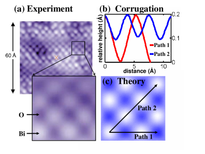
Figure 5: (a) Typical experimental topographical STM map after Ref. Pan, . (b) The computed corrugation of two STM line scans and (c) theoretically predicted topographic map. The two paths are shown in (c) by arrows.

We discuss first the topographic STM map, i.e., the constant current surface for a tip scanning across the sample surface. The computed topographic map is very robust against changes in measuring parameters such as the bias voltage or the tip-surface distance. Figure 5 compares the calculated and typical experimental results. Furthermore, corrugation along two paths of line scan is shown in Fig. 5 (b). The Bi atoms are seen as bright spots, while the surface oxygens are dark due to very low current coming through these surface atoms. We will see in connection with the analysis of the tunneling channels below that the apical oxygens act as the primary gate for passing electrons from the CuO₂ layers up to the surface BiO layer. Accordingly, the Bi atoms appear bright because there exists an easy channel between the surface Bi atoms and the apical oxygens below via the Bi $p_{z}$ orbitals. On the other hand, the oxygens in the surface layer are dark because the $p_{x,y}$ orbitals of O(Bi) are orthogonal to the (assumed) $s$-symmetry of the tip, while the O(Bi) $p_{z}$ orbitals are relatively weakly coupled to the $p_{z}$ of the apical oxygen as discussed below in connection with Fig. 7.

III.2 Tunneling spectra

Fig. 6 (a) compares a typical experimental (red line) STS spectrumMcElroy to the calculated one (black line). The overall agreement between theory and experiment is seen to be good, although the VHSs are seen as separate structures in the calculated curve footnote2 ; MSB . The agreement also extends to the low energy region shown in Fig. 6(b), where the width and positions of the coherence peaks is reproduced reasonably well.footkpoints The tendancy for increasing intensity towards negative bias is seen in both measurements and computations. This is in sharp contrast to the shape of the LDOS of Cu-$d_{x^{2}-y^{2}}$ orbital (green curve). As emphasized in Ref. NLMB , this remarkable asymmetry of the spectrum between positive and negative bias voltages reflects the opening up of channels other than Cu-$d_{x^{2}-y^{2}}$, especially of Cu-$d_{z^{2}}$, as one goes to high negative bias. This asymmetry thus appears naturally within our conventional picture and cannot be taken to be a hallmark of strong correlation effects as has been thought to be the case.

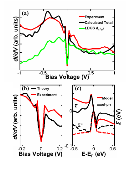
Figure 6: (color online) (a) A typical experimental tunneling spectrum (red line) from Bi2212 (after Ref. McElroy, ) is compared with the calculated spectrum (black). The green curve shows the LDOS of the Cu-$d_{x^{2}-y^{2}}$. (b) Expanded view of the experimental and calculated spectrum in the low energy region. (c) Comparison of the model self-energy (Eq. (19)) assumed for the Cu-$d_{x^{2}-y^{2}}$ orbitals and the self-energy from the convolution of a Debye-type phonon spectrum and the LDOS of Cu-$d_{x^{2}-y^{2}}$ (Eq. (18)) as discussed in Appendix A.

There has been considerable interest in understanding the coupling of electrons to bosonic modes in the so-called ‘low-energy kink’ region within $\sim\pm 100$ meV of the Fermi level. In particular, the peak-dip-hump structure seen in the experimental spectrum in Fig. 6(b) is generally believed to be the result of the coupling of electronic degrees of freedom to a collective mode (Refs. kinks, ; hoogenboom, ; VHS, ). Fig. 6(b) shows that the peak-dip-hump feature can be described by our simple self-energy correction discussed in Appendix A. This point however requires further study, including an analysis of how this feature evolves with doping.

III.3 Selection rules

The filter function $M_{tc}$ controls selection rules dictated by matching of the symmetry properties of the cuprate layer, filter layers and the tip. A closer examination of $M_{tc}$ reveals that strong tunneling through the apical oxygen layer is associated with a matching of the symmetry of the cuprate layer wave function to that of the apical O-$p_{z}$. The key is the relative symmetry of the wave functions with respect to the axis of tunneling: An ‘odd’ wave function, e.g., the Cu-$d_{x^{2}-y^{2}}$ has zero overlap with an ‘even’ wave function such as O-$p_{z}$. In contrast, two orbitals with the same symmetry couple more strongly. Accordingly, the $p_{z}$ of the apical oxygen and the Cu-$d_{z^{2}}$ possess large overlap, while Cu-$d_{x^{2}-y^{2}}$ has zero overlap with any $s$- or $p$-orbital of the apical oxygen. This is the reason that direct tunneling is forbidden between Cu-$d_{x^{2}-y^{2}}$ and the $s$-wave symmetric tip through the filter layer. Hence, $M_{tc}$ functions here are consistent with the filter function of Ref. Balatsky, . Similarly, coupling between an $s$-wave tip and the $p_{x}$ and $p_{y}$ orbitals of the Bi atom lying directly below the tip is forbidden. Therefore, within the filter layer, the main ‘vertical’ overlap is between the $p_{z}$ orbitals of Bi and apical oxygen, and these orbitals indeed are found to provide the main channel through the filter layers as depicted in Fig. 7(a). We find additional relatively small contributions from the on-site Bi-$s$-orbital and $p$-orbitals of the surrounding Bi and O(Bi) atoms, but such ’background’ contributions to the current do not seem to be dominated by any particular channel.

Figure 7(b) illustrates another example of a symmetry-forbidden tunneling path, where the tip is centered between two surface Bi’s, i.e. on the top of an oxygen of the cuprate layer. Since we assume an $s$-wave tip with negative hopping integrals to the nearby Bi atoms, when we follow either path up to the Cu-$d_{z^{2}}$ orbitals, the signs of the hopping integrals are identical. However, the O-$p_{x}$ orbital between the two Cu atoms changes sign from one Cu to the other. This gives the two paths from O-$p_{x}$ to the $s$-wave tip an opposite phase leading to destructive interference between the paths, making the O atom invisible. However, if the $s$-wave tip is replaced by one with, e.g, $p_{x}$ symmetry, the oxygen would become visible and a weaker signal would appear from the neighboring $d_{x^{2}-y^{2}}$ orbitals. Experimentally, this could be accomplished by functionalizing the tip by attaching a suitable molecule to the tip. A similar procedure has been used to obtain a contrast inversion for CO molecules adsorbed on a Cu surface Rieder ; Niemi1 .

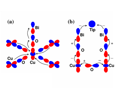
Figure 7: (color online) (a) Dominant tunneling channel from the cuprate layer, from Cu $d_{x^{2}-y^{2}}$ orbitals through the neighboring Cu $d_{z^{2}}$ to Bi $p_{x}$ to the tip. (b) An oxygen atom in the cuprate layer is invisible to a STM tip right above, since the paths through Cu₁ and Cu₂ interfere destructively.

III.4 Tunneling channels

The origin of the current from the cuprate layer can be understood by inspecting the individual terms of Eq. (17), which we refer to as ’tunneling channels’, i.e., from the regular and anomalous elements $G_{c\alpha}^{+}\Sigma{{}^{\prime\prime}}_{\alpha}G_{\alpha c^{\prime}}^{-}$ and $F_{c\alpha}^{+}\Sigma{{}^{\prime\prime}}_{\alpha}F_{\alpha c^{\prime}}^{-}$, of the Green’s function. [Although tunneling channels are a normal state property, the anomalous matrix elements play an important role in generating the coherence peaks and thus are relevant more generally.] For simplicity, we assume that the tip is right above a Bi atom. The dominant element of the filter function $M_{t,c}$ is then between the tip orbital and the $d_{z^{2}}$ orbital of the upper layer Cu atom lying beneath the surface Bi atom, so we take $c=c^{\prime}=$ Cu-$d_{z^{2}}$ in results shown in Figs. 8 and 9. Fig. 8 shows the relative contributions of the regular and anomalous matrix elements. The near Fermi energy current is primarily associated with the $d_{x^{2}-y^{2}}$ matrix elements. While the regular matrix elements of Cu-$d_{x^{2}-y^{2}}$ are almost solely responsible for the spectrum at energies around the VHSs, the anomalous elements determine the features around the gap region, especially the coherence peaks. Fig. 8 shows that coherence peaks are inherited from the anomalous and not the regular part of the Green’s function, and reflect physically the effects of non-conservation of the number of electrons near the gap region.

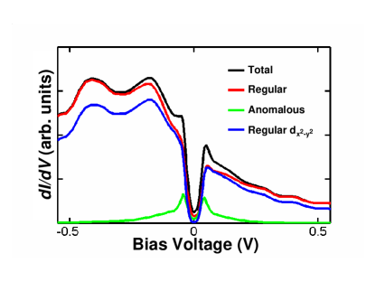
Figure 8: (color online) Partial spectrum with $c=c^{\prime}=d_{z^{2}}$ in $M_{tc}.$ The regular (red line) and anomalous (green line) components are shown together with the total contribution of the two parts (solid black). Blue curve shows the corresponding regular Cu-$d_{x^{2}-y^{2}}$ contributions.

In Fig. 9, the current of $d_{x^{2}-y^{2}}$ character is further broken down into contributions from various neighbors of the central Cu atom of the first and second CuO₂ layer away from the free surface. We see in panel (a) that the upper CuO₂ layer is more important than the lower one, but that the upper layer is by no means dominant. It seems that the coupling between the tip and the lower layer is strengthened via the relatively large overlap between the $d_{z^{2}}$ orbitals of the central Cu atoms of the two layers, which opens an important interlayer channel. The $d_{x^{2}-y^{2}}$ orbitals of the two layers mix not only to induce the well-known bilayer splitting in Bi2212, but also play a significant role in the flow of current to the tip from the lower cuprate layer.

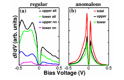
Figure 9: (color online) (a) Various contributions to tunneling spectrum from the regular matrix elements (assuming $c=c^{\prime}=d_{z^{2}}$ in $M_{tc}$), $T^{R}_{t\alpha}$, of Cu-$d_{x^{2}-y^{2}}$ orbitals of upper and lower CuO₂ layer. Contributions from the nearest neighbor (nn) Cu atoms in the upper and lower layer are shown. (b) Same as (a), except this panel refers to the contributions from the anomalous matrix elements, $T^{A}_{t\alpha}$.

It can be seen from Fig. 9 (a) that the $d_{x^{2}-y^{2}}$ orbitals of the four nearest-neighbor Cu atoms of the central Cu give a significant contribution to the total spectrum, but that this amounts to only about one third of the contribution from all $d_{x^{2}-y^{2}}$ terms from the upper layer. Due to the non-local nature of the Bloch-states within the cuprate layers, it is clear then that the total signal involves long range contributions, and attributing the spectrum merely to the four nearest neighbor Cu atoms provides only a rough approximation.

Anomalous contributions are considered in Fig. 9 (b). Here, the upper and lower layers give an almost equally large contribution, indicating that coherence peaks also are not all that local in character. Notably, we find a finite onsite anomalous contribution of $d_{x^{2}-y^{2}}$ even though the regular term is zero. This can be understood with reference to Eq. (6). Consider the term

$$F_{z^{2}d}=G_{e,z^{2}(d+x_{i})}^{0}\Delta_{(d+x_{i})d}G_{h,dd},$$

where $d$ is shorthand for $d_{x^{2}-y^{2}}$ of the central Cu and $d+x_{i}$ is $d_{x^{2}-y^{2}}$ of the neighboring Cu in either $x$- or $y$-direction. Clearly, $G_{e,z^{2}(d+x_{i})}^{0}$ transforms under rotations of $\frac{\pi}{2}$ in the same way as $\Delta_{(d+x_{i})d},$ and since $G_{h,dd}$ is an onsite term, the combination is invariant. Hence the four terms in the sum over the neighbors are equal, yielding a non-zero onsite term.

We emphasize that the anomalous contribution of the four neighboring Cu atoms is quite small. Let us consider the term

$$F_{z^{2}(d+x_{i})}=G_{e,z^{2}d}^{0}\Delta_{d(d+x_{i})}G_{h,(d+x_{i})(d+x_{i})}.$$

Due to symmetry, $G_{e,z^{2}d}^{0}=0,$ and thus this term vanishes. However, there are terms like

$$F_{z^{2}(d+x_{i})}=G_{e,z^{2}(d+2x_{i})}^{0}\Delta_{(d+2x_{i})(d+x_{i})}G_{h,(d+x_{i})(d+x_{i})}$$

which do not vanish, but are very small, since $G_{e,z^{2}(d+2x_{i})}^{0}$ is a relatively small term. A similar analysis can be carried out for the second and third neighbors. The second nearest neighbors, which lie along the nodal direction in k-space, give the largest single contribution, although this contribution is not dominant. The third neighbor contribution is a little larger than the onsite contribution.

IV Further Comments

IV.1 Symmetry Analysis

The selection rules can be formalized using group theoretical arguments related to the filtering function. Balatsky . For example, in order to explain the dominance of the $d_{x^{2}-y^{2}}$ orbitals of the four neighboring Cu atoms, considering representations of the two-dimensional $C_{4v}$ group, the d-orbitals $|d_{x^{2}-y^{2}},i\rangle$ of the site $i$ participate in eigenfunctions of the system as a linear combination

$${\sum_{i}}e^{-i\mathbf{k}\cdot\mathbf{R}_{i}}|d_{x^{2}-y^{2}},i\rangle.$$

This combination of the four neighboring orbitals at $(0,\pm\pi)$ and $(\pm\pi,0)$ belongs to the same representation of $C_{4v}$ as the $4s$ and $d_{z^{2}}$ orbitals of the central Cu atom (see Fig. 10), as well as the $p_{z}$ orbitals of the apical oxygen and the surface Bi atom. At this k-point, the phase difference between the lattice sites causes all the d-orbital lobes pointing towards the central atom to have the same sign. Hence, this combination yields a large off-diagonal element overlap with the surface $p_{z}$-orbital, and a dominant tunneling contribution around the gap. Similar arguments can be applied to understand contributions from other farther out atoms. An example was given in Fig. 7(b) above where the position of the tip and the symmetry of the relevant orbital strongly influence the visibility of an atom.

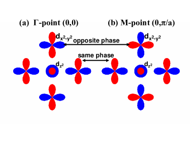
Figure 10: (color online) Relative phases of the central $d_{z^{2}}$ orbital and the neighboring $d_{x^{2}-y^{2}}$ orbitals at the $\Gamma$ point (a) and at the $M$ point (b).

IV.2 Electron extraction/injection

To relate the tunneling current to the LDOS of the cuprate layer, we have introduced the concept of tunneling paths through Eq. (14), which implies that each path begins or ends on a particular atomic orbital. This non-intuitive concept requires some comment. In reality, the current flows through the sample with each electron ejected to the tip being replaced by an electron from a distant counterelectrode. For a simple system, such as a nanostructure, non-equilibrium Green’s function formalism with two ‘leads’ closing a current circuit have been invoked (see, e.g., Ref. Meir, ). Tersoff-Hamann (TH) or Todorov-Pendry (TP) approach, on the other hand, assumes that the current is composed of a series of tunneling eventsTHTPfoot , and that the replacement of electrons at the counterelectrode has a negligible effect on the tunneling process. Since the current in STS is of the order of $10-100pA$, there is only about one electron each $1-10ns$ which flows across the sample, justifying the assumptions underlying TH/TP approach. Both TH and TP are based on calculating individual tunneling events in a LEED-like formalismShenRMP . Due to the finite $\Sigma"$, an electron created on a particular atom will have only a finite probability of escaping to the tunneling tip, and Eq. (14) shows how to add up the contribution of all these tunneling processes in terms of the equilibrium LDOS of the sample.

V Conclusions

We have presented a comprehensive framework for modeling the STS spectra from the normal as well as the superconducting state of complex materials in a material-specific manner. Our formulation makes transparent the connection between the LDOS and the STS spectrum or the nature of the tunneling ’matrix element’, and it is cast in a form that reveals the filtering effect of the overlayers separating the tip and the layers of interest. Our decomposition of the tunneling current into contributions from individual local orbitals allows us to identify important ’tunneling channels’ or paths through which current reaches the STM tip in the system. Our analysis highlights the importance of anomalous terms of the Green’s function, which account for the formation and breaking up of Cooper pairs, and how such terms affect the STS spectrum.

We apply the formalism to the specific case of Bi2212. Mismatch of symmetry between orbitals on adjacent atoms, or between the tip and the sample orbitals, is shown to severely restrict the corresponding contribution to the tunneling current. For these reasons, the contribution from Cu-$d_{x^{2}-y^{2}}$ orbitals comes not directly from the Cu-atom lying right below the Bi atom, but from a fourfold symmetric indirect route involving the four nearest-neighbors of the central Cu as well as longer range background from farther out Cu-$d_{x^{2}-y^{2}}$ orbitals. In the superconducting state, the coherence peaks of the spectrum are shown to be dominated by the anomalous spectral terms, which also are found not to be all that localized around the central Cu atom. In particular, we find a small anomalous on-site term and a practically vanishing first nearest neighbor contribution, with most of the anomalous contribution arising from the second neighbors and beyond.

We have concentrated in this study on the large hole doping regime of the cuprates where a homogeneous electronic Fermi liquid phase is consistent with most experiments. The fact that we have obtained good overall agreement between our computations and the measurements, especially with respect to the pronounced asymmetry of the spectrum between positive and negative bias voltages, indicates that this remarkable asymmetry can be understood more or less within our conventional picture without the need for invoking exotic mechanisms. At lower dopings, strong correlation effects including the possible presence of competing orders or inhomogeneous electronic states (nanoscale phase separation) would need to be taken into account. However, the present framework can be extended fairly straightforwardly through the addition of Hubbard terms in the Hamiltonian to provide a viable scheme for investigating the tunneling response throughout the phase diagram of the cuprates and other complex materials, including the modeling of effects of impurities and dopant atoms in the system.

Acknowledgments

This work is supported by the US Department of Energy, Office of Science, Basic Energy Sciences contract DE-FG02-07ER46352, and benefited from the allocation of supercomputer time at NERSC, Northeastern University’s Advanced Scientific Computation Center (ASCC), and the Institute of Advanced Computing, Tampere. RSM’s work has been partially funded by the Marie Curie Grant PIIF-GA-2008-220790 SOQCS. I.S. would like to thank the Wihuri Foundation for financial support. Conversations with Jose Lorenzana and Matti Lindroos are gratefully acknowledged.

Appendix A Boson-electron coupling

In the vicinity of the Fermi energy, dispersion anomalies are found in ARPES spectra arising from coupling of electronic degrees of freedom to phonons and/or magnetic modes, often giving the appearance of a peak-dip-hump featurekinks . These boson-electron couplings also strongly affect the STS spectrumVHS . This appendix discusses a model self-energy for describing such anomalies.

A significant contribution to the electron-phonon coupling is associated with modulation of the electronic hopping integrals by the phonons. The generalized coordinate of atomic displacement in $q$-basis is quantized in the standard way:

$$Q_{q}=\sqrt{\frac{\hbar}{2\Omega_{q}}}\left(a_{q}+a^{\dagger}_{q}\right),$$

where $a_{q}(a^{\dagger}_{q})$ is the annihilation (creation) operator of the phonon mode $q$, and $\Omega_{q}$ is the frequency of the mode. However, the most natural way to couple this to real-space tight-binding basis is to make a transformation to the basis of real space displacement of atom $\mu$ in the following way:

$$\hat{u}_{\mu}=\langle\mu|q\rangle Q_{q},$$

where Einstein summation over phonon modes $q$ is implicit. Note, that $\mu$ is a composite index denoting both the index of an atom and the direction of displacement.

Consequently, in tight-binding basis, this gives rise to a term in the Hamiltonian of the form

$$H^{el-vib}=\frac{1}{\sqrt{m_{\mu}}}\frac{\partial V_{\alpha\delta}}{\partial R_{\mu}}\hat{u}_{\mu}c^{\dagger}_{\alpha}c_{\beta}=\Gamma_{\mu}^{\alpha\delta}\hat{u}_{\mu}c^{\dagger}_{\alpha}c_{\beta}$$

where $V_{\alpha\delta}$ is the hopping integral between orbitals $\alpha$ and $\delta$, $R_{\mu}$ is the coordinate of atom $\mu$.

This coupling can be embedded into the electronic Hamiltonian as an energy dependent self-energy. Following the arguments of Ref. paulsson-05, , the general form of self-energy is written as:

$$\Sigma^{\pm}_{\alpha\beta}(\varepsilon)=\frac{\hbar}{2}\Gamma_{\mu}^{\alpha\delta}\Gamma_{\nu}^{\gamma\beta}\int d\Omega\frac{1}{\Omega}g_{\mu\nu}(\Omega)$$

$$((1-f(\varepsilon-\hbar\Omega)+n_{b}(\Omega))G_{\delta\gamma}^{\pm}(\varepsilon-\hbar\Omega)$$

$$+(f(\varepsilon+\hbar\Omega)+n_{b}(\Omega))G_{\delta\gamma}^{\pm}(\varepsilon+\hbar\Omega)),$$ (18)

where $g_{\mu\nu}(\Omega)=\sum_{q}\langle\mu|q\rangle\delta(\Omega-\Omega_{q})\langle q|\nu\rangle$ is an element of the vibration mode density matrix. Note again that we use Einstein summation convention, so that summation is implied over orbital indices $\gamma$ and $\delta$ and the phonon polarization indices $\mu$ and $\nu.$

For simplicity, we now assume that: (i) The bosonic coupling only affects the Cu-$d_{x^{2}-y^{2}}$ orbitals, where we include a diagonal self-energy of the form, $g(\Omega)=g\Omega^{2}$ when $\Omega\leq\Omega_{d}$ and it is 0 when $\Omega>\Omega_{d}$. For a Debye spectrum of phonons, $\Omega_{d}$ is the Debye cut-off frequency, and the normalization factor is $g=3/\Omega_{d}^{3}$; (ii) $\rho_{\delta\gamma}=-\frac{1}{\pi}Im[G^{+}_{\delta\gamma}]=\rho$ is approximately a constant. This amounts to assuming that the electronic density of states is smoothly varying within the range of the phononic spectrum; (iii) Take $\Gamma_{\mu}^{\alpha\delta}=\Gamma$, a constant parameter. Using these assumptions, the final form for the self-energy is

$$\Sigma^{+}=-\frac{A}{\pi}\left((2z+i\pi)+\left(z^{2}-1\right)\ln{\left(\frac{z-1}{z+1}\right)}\right),$$ (19)

where $z=(\varepsilon+i\eta)/(\hbar\Omega_{d})$, $A=\frac{3\hbar}{4\Omega_{d}}\Gamma^{2}\rho,$ and $\eta$ is a convergence parameter. Although we have derived the preceding form for coupling to a 3D Debye spectrum of phonons, the results are not too sensitive to details of the spectrum, and we would expect a similar result for an Einstein phonon or the magnetic resonance modemagres .

It is interesting to consider the asymptotic forms of self-energy as follows. If $\hbar\Omega_{d}\ll\varepsilon$,

$$\Sigma(\varepsilon)\approx-A\left(\frac{2}{\pi z}+i\right)$$

For large boson energies, i.e., $\hbar\Omega_{d}\gg\varepsilon$, we obtain

$$\Sigma(\varepsilon)\approx-A\left(\frac{4}{\pi}z+iz^{2}\right).$$ (20)

While Eq. (18) gives a general form of phononic self-energy for any pair of orbitals, in the present calculations, we adopt a few simplifications. First, we assume only diagonal terms of self-energy to make the model more tractable. Second, we apply Eq. (19) to Cu-$d_{x^{2}-y^{2}}$ orbitals using parameters $\hbar\Omega_{d}=80meV$ and $A=60meV.$ The former value gives the best fit to the peak-dip-hump structure, and the latter controls the smoothness of the spectrum. In Fig. 6(c) we make a comparison between the more general form of Eq. (18) with the accurate density of states of Cu-$d_{x^{2}-y^{2}}$ orbitals. For the remaining orbitals we mimic a Fermi-liquid type self-energy, which can be modeled with a $\Sigma^{\prime\prime}\propto\varepsilon^{2}$ and $\Sigma^{\prime}\propto\varepsilon$; here we employ the asymptotic form of Eq. (20), choosing parameters $\hbar\Omega_{d}=2.0eV$ (to ensure the correct asymptotic form for whole the energy range) and $A=100meV.$ In this way, the need for a Kramers-Kronig transformation is avoided.

We can straightforwardly include in the self-energy the effect of magnon scatteringMSB responsible for the high energy kinkHEK . This will broaden the spectrum in the vicinity of the VHS peaks, thereby improving agreement with experiment in Fig. 6(a). It should be noted, however, that a more accurate modeling of the self-energy will be required both for the bosonic coupling and the Fermi-liquid term for treating the underdoped system.

Appendix B Bogoliubov quasiparticles in tight-binding basis

This appendix discusses aspects of the Bogoliubov transformation within a tight-binding basis. The Bogoliubov transformation is not explicitly carried out in the present calculations since the Green’s function tensor is obtained directly from Dyson’s equation. Nevertheless, understanding the relation between the transformation and the Green’s function tensor in the tight-binding basis is necessary for interpreting some of our results. In particular, our analysis of pairing symmetry is based on the relation between $F_{\alpha\beta}$ and $\langle c_{\alpha\uparrow}c_{\beta\downarrow}\rangle.$

The Bogoliubov transformation bogoliubov is conventionally carried out in a combined basis of spin-up electrons and spin-down holes:

$$\mathbf{c}_{k}=\left(\begin{array}[]{c}c_{k\uparrow}\\ c^{\dagger}_{-k\downarrow}.\end{array}\right)$$ (21)

These $c$’s diagonalize the one-particle Hamiltonian of Eq. (1) via the transformations

$$c_{\alpha\uparrow}=\langle\alpha|k\rangle c_{k\uparrow}$$

and

$$c^{\dagger}_{\alpha\downarrow}=\langle-k|\alpha\rangle c^{\dagger}_{-k\downarrow}=\langle\alpha|k\rangle c^{\dagger}_{-k\downarrow},$$

or in a more compact form:

$$\mathbf{c}_{\alpha}=\left(\begin{array}[]{c}c_{\alpha\uparrow}\\ c^{\dagger}_{\alpha\downarrow}.\end{array}\right)=\left(\begin{array}[]{cc}\langle\alpha|k\rangle&0\\ 0&\langle\alpha|k\rangle\end{array}\right)\mathbf{c}_{k}=B_{\alpha k}\mathbf{c}_{k},$$ (22)

with inverse $\mathbf{c}_{k}=B_{k\alpha}\mathbf{c}_{\alpha}.$

This change of basis diagonalizes the one-particle Hamiltonian:

$$\varepsilon_{k}=\langle k|\alpha\rangle H_{1,\alpha\beta}\langle\beta|k\rangle$$

(with summation over $\alpha$ and $\beta$). In this basis the Hamiltonian of Eq. (3) becomes

$$H=\varepsilon_{k}c^{\dagger}_{k\uparrow}c_{k\uparrow}+\varepsilon_{k}(1-c_{-k\downarrow}c^{\dagger}_{-k\downarrow})+\Delta_{k}c^{\dagger}_{k\uparrow}c^{\dagger}_{-k\downarrow}+\Delta^{\dagger}_{k}c_{-k\downarrow}c_{k\uparrow},$$

now with summation over $k.$ After shifting this by a constant energy, it assumes the simple form

$$H^{eff}=\mathbf{c}^{\dagger}\hat{H}\mathbf{c},$$

where

$$\hat{H}=\left(\begin{array}[]{cc}\varepsilon_{k}&\Delta_{k}\\ \Delta^{\dagger}_{k}&-\varepsilon_{k}\end{array}\right),$$ (23)

which can be diagonalized into

$$H^{eff}=\mathbf{c}^{\dagger}U^{-1}U\hat{H}U^{-1}U\mathbf{c},$$

where

$$U=\left(\begin{array}[]{cc}u^{*}_{k}&v_{k}\\ -v^{*}_{k}&u_{k}\end{array}\right)~{}~{}\textrm{and}~{}~{}U^{-1}=\left(\begin{array}[]{cc}u_{k}&-v_{k}\\ v^{*}_{k}&u^{*}_{k}\end{array}.\right)$$

The coefficients are chosen in the standard way in order to obtain a diagonal matrix

$$U\hat{H}U^{-1}=\left(\begin{array}[]{cc}E_{k}&0\\ 0&-E_{k}\end{array}\right),$$

with $E_{k}=\sqrt{\varepsilon_{k}^{2}+|\Delta_{k}|^{2}}.$

This Bogoliubov transformation introduces the quasi-particle basis

$$\mathbf{a}=\left(\begin{array}[]{c}a_{k}\\ b^{\dagger}_{-k}\end{array}\right)=U\mathbf{c}.$$

Since we are working in the tight-binding basis, we end up with

$$\left(\begin{array}[]{c}a_{k}\\ b^{\dagger}_{-k}\end{array}\right)=\left(\begin{array}[]{cc}u^{*}_{k}\langle k|\alpha\rangle&v_{k}\langle k|\beta\rangle\\ -v^{*}_{k}\langle k|\alpha\rangle&u_{k}\langle k|\beta\rangle\end{array}\right)\left(\begin{array}[]{c}c_{\alpha\uparrow}\\ c^{\dagger}_{\beta\downarrow}\end{array}\right)$$

(summation over $\alpha$ and $\beta$) or inversely

$$\left(\begin{array}[]{c}c_{\alpha\uparrow}\\ c^{\dagger}_{\beta\downarrow}\end{array}\right)=\left(\begin{array}[]{cc}\langle\alpha|k\rangle u_{k}&-\langle\alpha|k\rangle v_{k}\\ \langle\beta|k\rangle v^{*}_{k}&\langle\beta|k\rangle u^{*}_{k}\end{array}\right)\left(\begin{array}[]{c}a_{k}\\ b^{\dagger}_{-k}\end{array}\right)$$

(summation over $k$).

We are particularly interested in writing the expectation values of electron and hole densities, $\langle c^{\dagger}_{\alpha\sigma}c_{\beta\sigma}\rangle,$ and $\langle c_{\alpha\sigma}c^{\dagger}_{\beta\sigma}\rangle,$ and pairing amplitudes $\langle c^{\dagger}_{\alpha\uparrow}c^{\dagger}_{\beta\downarrow}\rangle,$ and $\langle c_{\beta\downarrow}c_{\alpha\uparrow}\rangle$ in terms of the Green’s function tensor. For this purpose, we start with a $2\times 2$ tensor

$$\langle\mathbf{c}_{\alpha}\mathbf{c}^{\dagger}_{\beta}\rangle=\langle B_{\alpha k}\mathbf{c}_{k}\mathbf{c}^{\dagger}_{k}B_{k\beta}\rangle=\langle B_{\alpha k}U^{-1}\mathbf{a}\mathbf{a}^{\dagger}UB_{k\beta}\rangle.$$ (24)

Using the fact that $\langle a_{k}a^{\dagger}_{k}\rangle=1-f(E_{k})$ and $\langle b^{\dagger}_{k}b_{k}\rangle=f(E_{k})$, we evaluate each element of the tensor $\langle\mathbf{c}_{\alpha}\mathbf{c}^{\dagger}_{\beta}\rangle$ separately as follows:
(1) The number density

$$\langle c^{\dagger}_{\alpha\uparrow}c_{\beta\uparrow}\rangle=\langle\beta|k\rangle\left(|u|^{2}f(E_{k})+|v|^{2}(1-f(E_{k}))\right)\langle k|\alpha\rangle$$

Now we use a trick following Ref. Horsfield, where

$$\langle\beta|k\rangle|u|^{2}f(E_{k})\langle k|\alpha\rangle=\int d\varepsilon f(\varepsilon)\langle\beta|k\rangle u\delta(\varepsilon-E_{k})u^{*}\langle k|\alpha\rangle$$

and

$$\delta(\varepsilon-E_{k})\approx-\frac{1}{\pi}Im(\frac{1}{\varepsilon-E_{k}+i\eta}).$$

Hence

$$\langle\beta|k\rangle|u|^{2}f(E_{k})\langle k|\alpha\rangle=\int d\varepsilon f(\varepsilon)\rho^{e}_{\beta\alpha}(\varepsilon),$$

where

$$\rho^{e}_{\beta\alpha}(\varepsilon)=-\frac{1}{\pi}Im(G^{+}_{e,\beta\alpha}(\varepsilon)),$$

where $G^{+}_{e,\beta\alpha}$ refers to the electron part of the Green’s function,

$$G^{+}_{e,\alpha\beta}(\varepsilon)=\frac{\langle\alpha,e|k\rangle\langle k|e,\beta\rangle}{\varepsilon-E_{k}+i\eta}=\frac{\langle\alpha|k\rangle|u_{k}|^{2}\langle k|\beta\rangle}{\varepsilon-E_{k}+i\eta}.$$

It is straightforward to show that

$$\langle c^{\dagger}_{\alpha\uparrow}c_{\beta\uparrow}\rangle=\int d\varepsilon[f(\varepsilon)\rho^{e}_{\beta\alpha}(\varepsilon)+(1-f(\varepsilon))\rho^{h}_{\beta\alpha}(\varepsilon)],$$

where $\rho^{h}_{\alpha\beta}$ is the hole density matrix. The first part of the integral, in fact, gives the number of electrons with a chosen spin. The latter part gives the same result as the former since the Bogoliubov transformation reflects the electron bands to hole bands with respect to the Fermi energy;
(2) The pairing amplitude

$$\langle c_{\alpha\uparrow}c_{\beta\downarrow}\rangle=\langle\alpha|k\rangle\left(u(f(E_{k})-(1-f(E_{k}))v\right)\langle k|\beta\rangle.$$

Using the trick of Ref. Horsfield, again gives us the formula

$$\langle c_{\alpha\uparrow}c_{\beta\downarrow}\rangle=-\int d\varepsilon(1-2f(\varepsilon))\rho^{eh}_{\alpha\beta}(\varepsilon),$$ (25)

where

$$\rho^{eh}_{\alpha\beta}(\varepsilon)=-\frac{1}{\pi}Im(F^{+}_{\alpha\beta}(\varepsilon)),$$

and

$$F^{+}_{\alpha\beta}(\varepsilon)=\frac{\langle\alpha,e|k\rangle\langle k|h,\beta\rangle}{\varepsilon-E_{k}+i\eta}=\frac{\langle\alpha|k\rangle u_{k}v_{k}\langle k|\beta\rangle}{\varepsilon-E_{k}+i\eta}$$

In the same manner, one can see that

$$\langle c^{\dagger}_{\alpha\uparrow}c^{\dagger}_{\beta\downarrow}\rangle=-\int d\varepsilon(1-2f(\varepsilon))\rho^{eh\dagger}_{\beta\alpha}(\varepsilon),$$ (26)

where

$$\rho^{eh\dagger}_{\beta\alpha}(\varepsilon)=-\frac{1}{\pi}Im((F^{+})^{\dagger}_{\beta\alpha}(\varepsilon)),$$

Equations (25) and (26) also reveal how the anomalous part of the Green’s function tensor is related to the pairing amplitude $\langle c_{\alpha\uparrow}c_{\beta\downarrow}\rangle$ in a tight-binding basis, or equivalently how the anomalous part of the current is related to the making and breaking of Cooper pairs. In particular, symmetry properties of $F_{\alpha\beta}$ are seen to be related directly to those of $\langle c_{\alpha\uparrow}c_{\beta\downarrow}\rangle$.

References

- (1) Ø. Fischer, M. Kugler, I. Maggio-Aprile, and Chr. Berthod, and Chr. Renner, Rev. Mod. Phys. 79, 353 (2007).
- (2) K. McElroy, Jinho Lee, J.A. Slezak, D.-H. Lee, H. Eisaki, S. Uchida, and J.C. Davis, Science 309, 1048 (2005).
- (3) E.W. Hudson, K.M. Lang, V. Madhave, S.H. Pan, H. Eisaki, S. Uchida, and J.C. Davis, Nature 411, 920 (2001).
- (4) S.H. Pan, E.W. Hudson, K.M. Lang, H. Eisaki, S. Uchida, and J.C. Davis, Nature 403, 746(2000).
- (5) A.N. Pasupathy, A. Pushp, K.K. Gomes, C.V. Parker, J. Wen, Z. Xu, G. Gu, S. Ono, Y. Ando, and A. Yazdani, Science 320, 196 (2008).
- (6) A.V. Balatsky, , A. V., Vekhter, I., and Zhu, J.-X., Rev. Mod. Phys. 78, 373 (2006).
- (7) Y. Kohsaka, C. Taylor, K. Fujita, A. Schmidt, C. Lupien, T. Hanaguri, M. Azuma, M. Takano, H. Eisaki, H. Takagi, S. Uchida, and J.C. Davis, Science 315, 1380 (2007).
- (8) I. Martin, A.V. Balatsky, and J. Zaanen, Phys. Rev. Lett. 88, 097003 (2002).
- (9) B.W. Hoogenboom, C. Berthod, M. Peter, Ø. Fischer, and A.A. Kordyuk, Phys. Rev. B 67, 224502(2003).
- (10) J.A. Nieminen, H. Lin, R.S. Markiewicz, and A. Bansil, Phys. Rev. Lett. 102,037001 (2009).
- (11) T.N. Todorov, G.A.D. Briggs and A.P. Sutton, J.Phys.: Condens. Matter 5, 2389 (1993).
- (12) J.B. Pendry, A.B. Prêtre and B.C.H. Krutzen, J.Phys.: Condens. Matter 3, 4313 (1991).
- (13) J. Tersoff and D.R. Hamann, Phys. Rev. B 31, 805 (1985).
- (14) Note that the tunneling signal decays exponentially with layer distance from the tip, and therefore, we expect the results presented in this article to be essentially the same as for a semi-infinite solid.
- (15) V. Bellini, F. Manghi, T. Thonhauser, and C. Ambrosch-Draxl, Phys. Rev. B 69, 184508(2004).
- (16) J.C. Slater and G.F. Koster, Phys. Rev. 94, 1498 (1954).
- (17) W.A. Harrison, Electronic Structure and Properties of Solids. Dover, New York (1980).
- (18) L. Shi and D. A. Papaconstantopoulos, Phys. Rev. B 70, 205101 (2004).
- (19) A. Bansil and M. Lindroos, Phys. Rev. Lett. 83, 5154(1999).
- (20) M. Lindroos, S. Sahrakorpi and A. Bansil, Phys. Rev. B 65, 054514(2002)
- (21) A. Bansil, M. Lindroos, S. Sahrakorpi, and R.S. Markiewicz, Phys. Rev. B 71, 012503(2005).
- (22) R.S. Markiewicz, S. Sahrakorpi, M. Lindroos, Hsin Lin, and A. Bansil, Phys. Rev. B 72, 054519(2005).
- (23) M.C. Asensio, J. Avila, L. Roca, A. Tejeda, G. D. Gu, M. Lindroos, R. S. Markiewicz, and A. Bansil, Phys. Rev. B 67, 014519(2003).
- (24) A. Bansil and M. Lindroos, Journal of Physics and Chemistry of Solids 59, 1879(1998).
- (25) H. Lin, S. Sahrakorpi, R.S. Markiewicz, and A. Bansil, Phys. Rev. Lett. 96, 097001 (2006).
- (26) K. K. Gomes, A. N. Pasupathy, A. Pushp, S. Ono, Y. Ando, and A. Yazdani, Nature 447, 569-572(2007).
- (27) A. Kaminski et al., Phys. Rev. B 73, 174511(2006).
- (28) J.A. Nieminen and S. Paavilainen, Phys. Rev. B 60, 2921 (1999).
- (29) In practice, we calculate the Green’s function for each k-point separately to produce the site-dependent Green’s function by inverse Fourier-transformation: Here the shorthand notation, , is used in that indices and implicitly contain the simulation cell index. Note also, that the inverse transformation must not be done until solving the whole Green’s function tensor.
- (30) J.-M. Tang and M. E. Flatté, Phys. Rev. B 66, 060504(R) (2002); J.-M. Tang and M. E. Flatté, Phys. Rev. B 70, 140510(R) (2004).
- (31) A.L. Fetter and J.D. Walecka, Quantum Theory of Many-Particle Systems. Dover (2003).
- (32) F.C. Zhang and T.M. Rice, Phys. Rev. B 37, 3759(1988).
-
(33)
The d-wave and ZRS symmetries are
not uniquely determined by the present choice of pairing. For instance, we
could choose an onsite pairing at the oxygen orbitals
with
In that case, Eq. (6)
could be written in the -direction as,
with a corresponding expression in the -direction. If and , the sign of is totally determined by the product of the lobes of the orbitals of the neighboring Cu atoms. This is, however, invariant under rotation by , and thus, follows the symmetry of - (34) Y. Meir and N.S. Wingreen, Phys. Rev. Lett. 68, 2512 (1992).
- (35) H. Ness and A.J. Fisher, Phys. Rev. B 56, 12469 (1997).
- (36) T. Frederiksen, M. Paulsson, M. Brandbyge, and A.-P. Jauho, Phys. Rev. B 75, 205413 (2007).
- (37) In the present study, the decomposition of Eq. (8) into tunneling channels has been significantly elaborated beyond our recent work in Ref. NLMB, . The most significant improvement is the explicit formulation of anomalous tunneling channels. Furthermore, we can obtain the total contribution of any chosen orbital over the whole infinite slab via the relation to regular and anomalous terms of Eq. (17). Note that the simulation cell indices and are explicitly written in the left hand side.
- (38) M. Magoga and C. Joachim, Phys. Rev. B 59, 16011 (1999).
- (39) P. Sautet, Surf. Sci. 374, 374 (1997).
- (40) E. Niemi and J. Nieminen, Chem. Phys. Lett. 397, 200 (2004).
- (41) The distinct VHS peaks in the computed spectrum are expected to be broadened to yield a smooth hump much like the experimental spectrum due to self-energy corrections resulting from magnetic response of the electron gas in the -400 meV range. These self-energy corrections are not included in the present calculations.
- (42) R.S. Markiewicz, S. Sahrakorpi, and A. Bansil, Phys. Rev. B 76, 174514 (2007).
- (43) Note that in solving the Dyson’s equation, the initial Green’s function for each k-point is a diagonal matrix of complex Lorentzians. An infinite number of k-points would be required for a final Green’s function without any artificial “shoulders”, although the imaginary part of the self-energy acts to smooth away the unwanted structures.
- (44) A. Lanzara et al., Nature (London) 412, 510 (2001); X. J. Zhou et al., Phys. Rev. Lett. 95, 117001 (2005). A. Kaminski et al., Phys. Rev. Lett. 86, 1070 (2001); P. D. Johnson et al., ibid. 87, 177007 (2001); S. V. Borisenko et al., ibid. 90, 207001 (2003); A. D. Gromko et al., Phys. Rev. B 68, 174520 (2003).
- (45) G. Levy de Castro, Chr. Berthod, A. Piriou, E. Giannini, and Ø. Fischer, Phys. Rev. Lett. 101, 267004 (2008).
- (46) L. Bartels, G. Meyer and K.-H. Rieder. Appl. Phys. Lett. 71, 213 (1997).
- (47) J. Nieminen, E. Niemi, K.-H. Rieder, Surface Science 552, L47-L52 (2004).
- (48) Although TP and TH are formulated in terms of LDOS, both approaches can, in principle, be decomposed into a spectral function form since the density matrix can be decomposed in this way regardless of the basis set employed.
- (49) A.P. Shen, Rev. Mod. Phys. 4, 382 (1971).
- (50) M. Paulsson, T. Frederiksen, and M. Brandbyge, Phys. Rev. B 72, 201101(R) (2005).
- (51) Z.-X. Shen and J.R. Schrieffer, Phys. Rev. Lett. 78, 1771 (1997); M.R. Norman and H. Ding, Physical Review B 57, R11089 (1998); S. LaShell, E. Jensen, and T. Balasubramanian, Phys. Rev. B 61, 2371 (2000)
- (52) F. Ronning, K.M. Shen, N.P. Armitage, A. Damascelli, D.H. Lu, Z.-X. Shen, L.L. Miller, and C. Kim, Phys. Rev. B 71, 094518 (2005); J. Graf, G.-H. Gweon, K. McElroy, S.Y. Zhou, C. Jozwiak, E. Rotenberg, A. Bill, T. Sasagawa, H. Eisaki, S. Uchida, H. Takagi, D.-H. Lee, and A. Lanzara, Phys. Rev. Lett. 98, 067004 (2007).
- (53) M. Tinkham, Introduction to Superconductivity. McGraw-Hill International Editions (1996).
- (54) A.P. Horsfield, A.M. Bratkovsky, M. Fearn, D.G. Pettifor, and M. Aoki, Phys. Rev. B 53, 12694(1996).