Statistical Analysis of Galaxy Surveys-IV:
An objective way to quantify the impact of superstructures on galaxy clustering statistics

Abstract

For galaxy clustering to provide robust constraints on cosmological parameters and galaxy formation models, it is essential to make reliable estimates of the errors on clustering measurements. We present a new technique, based on a spatial Jackknife (JK) resampling, which provides an objective way to estimate errors on clustering statistics. Our approach allows us to set the appropriate size for the Jackknife subsamples. The method also provides a means to assess the impact of individual regions on the measured clustering, and thereby to establish whether or not a given galaxy catalogue is dominated by one or several large structures, preventing it to be considered as a “fair sample”. We apply this methodology to the two- and three-point correlation functions measured from a volume limited sample of M^∗ galaxies drawn from data release seven of the Sloan Digital Sky Survey (SDSS). The frequency of jackknife subsample outliers in the data is shown to be consistent with that seen in large N-body simulations of clustering in the cosmological constant plus cold dark matter cosmology. We also present a comparison of the three-point correlation function in SDSS and 2dFGRS using this approach and find consistent measurements between the two samples.

1 Introduction

The clustering of galaxies has the potential to place constraints on the values of fundamental cosmological parameters and to probe the efficiency of galaxy formation in dark matter haloes of different masses. A key assumption made when interpreting clustering measurements is that the sample used is representative of a much larger volume of the Universe. The hope is that the survey volume is sufficiently large that the clustering measurements made from it should agree with the mean of measurements obtained from an ensemble of similar volumes (which is, in general, not feasible to carry out). This is the “fair sample” hypothesis (Peebles 1980).

This “fair sample” hypothesis, commonly invoked in large scale structure analyses, is often abused in the literature. The hypothesis relies on two conditions: (a) that the clustering statistic for one survey is not biased with respect to the mean measurement from an ensemble of independent but similar surveys; (b) that the error estimate on the statistic is properly characterized, i.e. it accounts for the variance seen in the ensemble of measurements (that is most often not achievable with real data). The latter point is often ignored and samples are referred to as “unfair” when the clustering statistic (with its associated errors) is at odds with either that from other samples (and their errors) or with the expected, theoretical value. The point we want to stress in this paper is that most surveys are likely to be “fair” but that the associated error analysis is likely to be “unfair”. This problem arises because a simplistic (or computationally inexpensive) approach to estimating the errors has been implemented and insufficient attention has been given to the inherent limitations of the method used. The recent extensive use of covariance matrices to account for the full error budget has brushed aside the important discussion of the limitations of the error method considered (as discussed at length in e.g. Norberg et al. 2009 for 2-point clustering statistics).

Surveys of the local Universe have increased in size by several orders of magnitude since the late 1990s, with over one million galaxy redshifts measured to date, spanning volumes running to several hundreds of cubic megaparsecs (York et al. 2000; Colless et al. 2001, 2003). Nevertheless, some clustering analyses have thrown up unusual results which suggest that current surveys may not, at least under certain conditions, be fair samples of the Universe. These anomalous results were first revealed in the form of the hierarchical amplitudes, the ratio of higher order correlation functions to a power of the two-point function, measured from volume limited samples drawn from the two-degree field galaxy redshift survey (2dFGRS; Baugh et al. 2004; Croton et al. 2004; Gaztanaga et al. 2005). The hierarchical amplitudes measured from the 2dFGRS displayed an upturn on large scales which is not expected in the gravitational instability scenario (e.g. Baugh, Gaztanaga & Efstathiou 1995). Croton et al. (2004) demonstrated that this was due to two particularly “hot” cells in the cell count distribution, which contained unusually large numbers of galaxies. On blanking out these cells from the survey and removing them from the count probability distribution, the hierarchical amplitudes resembled the theoretical expectations more closely. Similar conclusions were reached in separate analyses of the two-point and three point correlation functions measured from the Sloan Digital Sky Survey (SDSS; Zehavi et al. 2002, 2004, 2005, 2011; Nichol et al. 2006; McBride et al. 2011a).

One of the “superstructures” identified in the 2dFGRS analyses is part of the SDSS “Great Wall” (Gott et al. 2005). Clustering measurements from the magnitude limited 2dFGRS do not show any significant change when this region is omitted (e.g. Cole et al. 2005). The influence of this structure over clustering measurments seems to depend on how the sample is constructed, an issue which we investigate further in this paper. The two point clustering analyses of Zehavi et al. (2002, 2005, 2011) on SDSS have shown explicitly the influence of the SDSS “Great Wall” on their measurments, with volume limited samples of M^∗ galaxies being particularly affected, whereas samples corresponding to brighter galaxy luminosities are less sensitive to the presence of this structure. Different volume limited samples will weight the structure differently, as it will be traced out by a different number of galaxies. Also, the volume of the sample changes when the luminosity defining it is varied; in a larger volume, other, similar structures may feature, diluting the impact of any single structure on clustering measurements.

Croton et al. (2004, 2007), as well as Gaztañaga et al (2005), presented measurements with and without the galaxies in the hot regions identified in their counts in cells analysis of the 2dFGRS, with the simple aim of showing the contribution of this structure on the hierarchical moments. Their approach was specific to the counts in cells clustering analysis. In this paper we present an objective technique which can be applied to any clustering statistic. The new method we describe is a development of the Jackknife technique for error estimation (see e.g. Norberg et al. 2009 for a review and application of this method and others to galaxy clustering error estimations; see also Zehavi et al. 2002 who gives the first comprehensive description of the Jackknife method for clustering statistics, which was used in the eariler clustering analysis of Roche et al. 1993 and Croft et al. 1999). Our approach can be used to assess whether or not a clustering signal is unduly influenced by the galaxy distribution in one particular region of a survey. Furthermore, we discuss a new statistic, the JK ensemble fluctuation, which provides a robust assessment of such fluctuations in the galaxy distribution. We note here that McBride et al. (2011a) present a similar analysis for their SDSS 3-point function measurement (in particular their Figs. 11, 12, and 13 are very relevant for the present paper). The main difference between their work and ours is that we take the study of the influence of extreme structure significantly further, by introducing a new statistic the JK ensemble fluctuation.

This paper is laid out as follows. In Section 2 we present the galaxy survey data used, which is the seventh data release of the SDSS, the associated completeness masks, the division of the SDSS into Jackknife regions (or JK quilts) and the clustering statistics used. Section 3 is devoted to our new objective method based on Jackknife resampling of the data, which is applied to the M^∗ SDSS sample, and shows the impact of large structures or “superstructures” on 2 and 3-point statistics in redshift space. A new statistic, the JK ensemble fluctuation, is introduced to quantify the importance of outliers. In Section 4 we illustrate the performance of this new statistic and show how it successfully identifies unusual regions in SDSS DR7 and sets their significance. In Section 5 apply our Jackknife approach to $\Lambda$CDM simulations to show that they display similar outliers to those seen in the data. In Section 6 we revist the 3-pt correlation function analysis of Gaztañaga et al. (2005), but this time using our new methodology based on the JK ensemble fluctuation. A summary is given in Section 7. Throughout we assume a standard cosmological model, with $\Omega_{\rm M}=0.25$, $\Omega_{\Lambda}=0.75$ and a value for the Hubble parameter of $h=H_{0}/(100\,{\rm km\,s}^{-1}{\rm Mpc}^{-1})$.

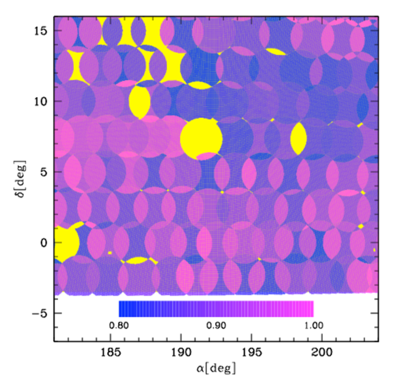
Figure 1: A zoomed in view of the SDSS redshift completeness mask. The colour bar indicates the redshift completeness fraction which ranges from 0.8 to 1. Sectors (i.e. uniquely defined regions sampled by the spectroscopic tiles) with completeness below 0.8 are shaded in yellow and regions outside the survey area in white.

2 Data and methodology

In this section we describe the galaxy data used (§ 2.1), the completeness mask of the survey (§ 2.2), the division of the survey into zones for Jackknife sampling (§ 2.3), the volume limited samples used in the clustering analysis presented in subsequent sections (§ 2.4) and the method estimation of 2 and 3 point correlation functions (§ 2.5).

2.1 SDSS DR7 Data

In this paper we use Data Release 7 (DR7) of the Sloan Digital Sky Survey (SDSS; Abazajian et al. 2009). DR7 covers 9380 deg² and contains 930 000 galaxy redshifts. We select galaxies brighter than a Petrosian magnitude of $r<17.65$. The magnitude limit is slightly brighter than that of the canonical main galaxy sample of $r=17.77$ (Strauss et al. 2002). We adopt this cut to avoid having to model a varying magnitude limit, which is needed to include all of the early SDSS data, since the magnitudes have been revised slightly since the early data were taken. In addition we also impose a bright magnitude limit of $r=15$, the point at which SDSS galaxy magnitudes start to become less reliable. The sample we consider contains 513k high quality, unique galaxy redshifts with a median redshift of $z_{\rm med}\simeq 0.10$. The precise choice of magnitude limit does not have an impact on our results. In our analysis we use SDSS Petrosian magnitudes calibrated using the prescription of Tucker et al. (2006) and corrected for Galactic extinction.

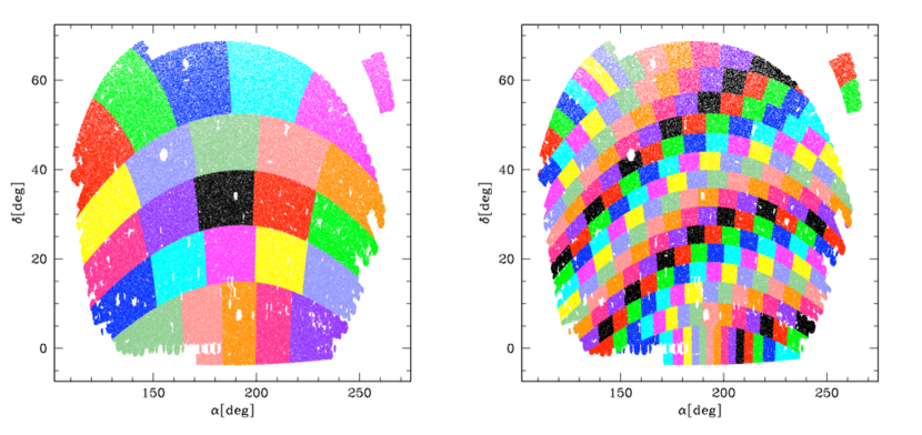
Figure 2: Left: The SDSS survey divided into 5x5 Jackknife regions in the $\alpha-\delta$ plane. The 25 zones in the resulting crazy quilt have equal area after taking into account their spectroscopic completeness. Right: Same as the left-hand panel, but for the case of 225 Jackknife zones corresponding to a square 15x15 Jackknife quilt.

2.2 SDSS survey mask

In order to make robust and reliable estimates of clustering the incompleteness in the spectroscopic catalogue needs to be taken into account. We do this using a redshift completeness mask. The variation in the survey completeness on the sky is then used to modulate the density of unclustered or random points used in the estimation of the mean density in clustering analyses.

We start by constructing a mask from the individual SDSS imaging scans. The imaging mask is pixelized using an equal-area projection, with a typical pixel area of $\sim 5.3$ arcmin². This is more than sufficient given the average number density of SDSS targets of $\sim 90$ galaxies deg^-2 and the typical scales we are interested in ($s\geq 1{\,h^{-1}\,{\rm Mpc}}$ at $z\geq 0.04$). Bad pixels, as labelled by the SDSS pipeline, are omitted from the imaging mask. Next, using the position of the spectroscopic tiles, we create the spectroscopic completeness mask, following the method devised for the 2dFGRS survey (Colless et al. 2001; Norberg et al. 2002; Cole et al. 2005). The survey is divided up into sectors which are regions defined by the unique overlap of spectroscopic tiles. Any sector which contains fewer than 10 galaxies is merged with its most populous neighbouring sector. This ensures that the sector completeness is not affected by shot-noise, which would lead to a patchy redshift completeness mask. The redshift completeness in a sector is the ratio of galaxies with a measured (high quality) spectroscopic redshift divided by the total number of galaxies in the target catalogue in that sector. The CasJobs SQL queries and data files used to retrieve the information required to construct the SDSS survey masks (imaging and spectroscopic) are given in Appendix A.

We show a small part of the survey mask we have constructed for the SDSS DR7 in Fig. 1. Regions outside the survey boundary are shaded white. Sectors which are less than 80% complete but which lie within the survey boundary are shaded yellow. The remaining sectors have a spectroscopic completeness ranging between 80 and 100%. It is these latter regions that are retained in our subsequent clustering analysis.

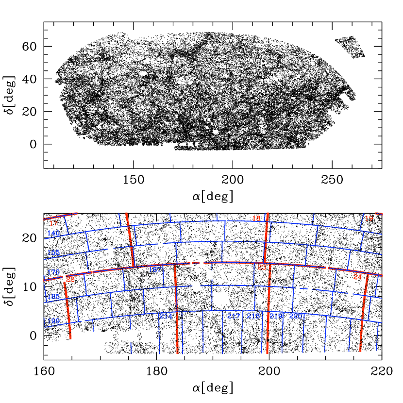
Figure 3: Top: The angular galaxy distribution of the ref volume limited sample (dots). Bottom: A zoomed in view centered on zone 23. Overplotted are the boundaries of the zones for the 5x5 and 15x15 Jackknife quilts, shown in thick red and thin blue linestyles respectively. The subzone numbers (colour coded according to the dimension of the quilt they belong to) are indicated for a limited number of patches, some of which will be referred to in later sections. The subzone number increases from left to right from top to bottom.

Table 1: A summary of the characteristics of the volume limited samples considered in this paper. Col. 1 - volume label ; col. 2 - absolute magnitude range ; col. 3 and 4 - minimum and maximum redshift limits respectively; col. 5 - sample volume; col. 6 - number of galaxies with redshift. Note that M^∗ is defined as in Blanton et al. (2003b), i.e. M^∗$-5\log_{10}h=-20.44$. The first three entries in the table correspond to approximately the same volume.

Label	M-range	$z_{min}$	$z_{max}$	V/${\,h^{-3}\,{\rm Mpc^{3}}}$	Ng
ref	M∗$+0.5\leq$M$\leq$M∗$-0.5$	0.0508	0.1065	(258.3)3	98 317
faint-ref	M∗$+0.5\leq$M$\leq$M∗	0.0405	0.1065	(263.5)3	63 916
bright-ref	M∗$\leq$M$\leq$M∗$-0.5$	0.0508	0.1065	(258.3)3	37 914
bright-all	M∗$\leq$M$\leq$M∗$-0.5$	0.0508	0.1325	(325.9)3	76 332
bright-far	M∗$\leq$M$\leq$M∗$-0.5$	0.1065	0.1325	(259.0)3	38 418

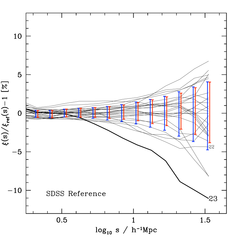
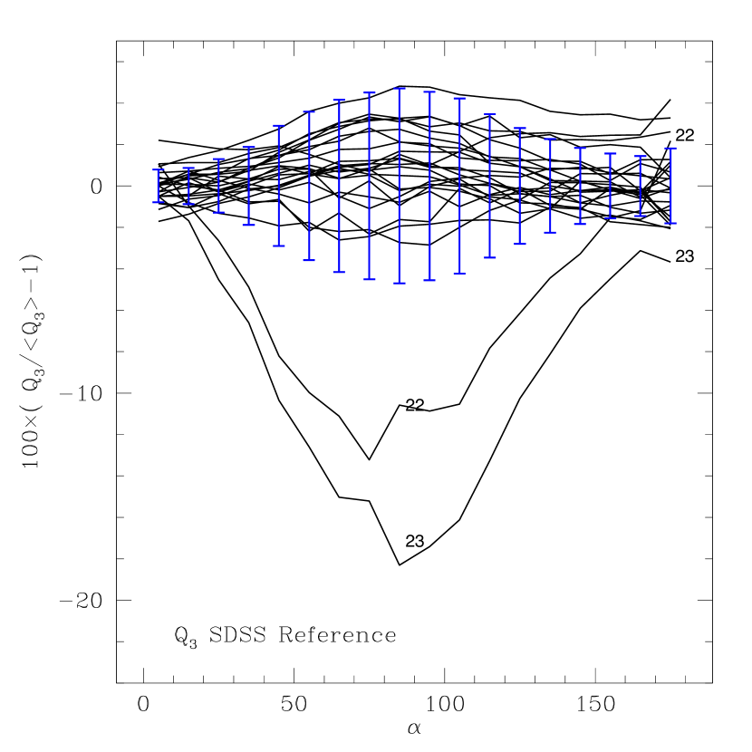
Figure 4: The distribution of clustering measurements from the Jackknife resamplings of the ref sample. The left-hand panel shows the measurements for $\xi(s)$ and the right-hand panel shows Q${}_{3}(\alpha)$, with $\alpha$ in degrees. In both cases, we plot the ratio of the correlation function measured from each Jackknife resampling to that measured from the full ref sample. The lowest amplitude correlation functions are labelled by the zone number omitted in the resampling. The larger (blue) errorbars show the rms error estimated from a Jackknife resampling of all of the zones, which corresponds to the central 68% of the distribution of measurements. In the left hand panel we also show the slightly smaller (red) errorbars, corresponding to the rms error estimated on omitting zone 23 from the Jackknife resampling altogether. Note that these errorbars are smaller by a factor $\sqrt{{\rm N_{\rm sub}}}$ than those assigned by Jackknife errors to correlation function measurements (see e.g. Eq. 1).

2.3 SDSS Jackknife quilts

Our goal in this paper is to assess the impact of unusual structures on clustering statistics. We do this by dividing the SDSS survey up into different regions to assess their contribution to the clustering signal. A framework in which to do this analysis is provided by the Jackknife approach to error estimation (see e.g. Norberg et al. 2009). In this method, a dataset is divided into $N_{\rm sub}$ zones. The clustering is then measured from a sample made up of $N_{\rm sub}-1$ of these zones, leaving one of the zones out. This process is repeated $N_{\rm sub}$ times, leaving out each one of the zones in turn. The scatter between the clustering measurements from the Jackknife samples is used to estimate the error on the clustering statistic. For completeness we quote here the standard relation used to estimate the Jackknife covariance matrix (see e.g. Norberg et al. 2009, Zehavi et al. 2002) when split into N_sub samples:

$$C_{\rm jk}(x_{i},x_{j}) = \frac{({\rm N_{\rm sub}}-1)}{{\rm N_{\rm sub}}}\sum_{k=1}^{{\rm N_{\rm sub}}}(x_{i}^{k}-\bar{x_{i}})(x_{j}^{k}-\bar{x_{j}})~{},$$ (1)

where $x_{i}$ is the $i^{\rm th}$ measure of the statistic of interest. It is assumed that the mean expectation value is given by

$$\bar{x_{i}} = \sum_{k=1}^{\rm N_{\rm sub}}x_{i}^{k}/{\rm N_{\rm sub}}\,,$$ (2)

but it can also be given simply by the measurement over the whole sample. Note the factor of ${\rm N_{\rm sub}}-1$ which appears in Eq. 1 (Tukey 1958; Miller 1974). Qualitatively, this factor takes into account the lack of independence between the N_sub copies or resamplings of the data; recall that from one copy to the next, only two sub-volumes are different (or equivalently ${\rm N_{\rm sub}}-2$ sub-volumes are the same).

Here we divide the SDSS survey into zones in right ascension and declination, producing what we call the survey “quilt”. The zones have equal areas after taking into account their spectroscopic completeness, using the completeness mask described above. We use square 5x5 (i.e. $N_{\rm sub}=25$ Jackknife zones) and 15x15 (i.e. $N_{\rm sub}=225$ Jackknife zones) Jackknife quilt patterns in the right ascension ($\alpha$) and declination ($\delta$) plane, leading to the quilt patchworks shown in Fig. 2. We also investigated Jackknife quilts with other dimensions (N_sub= 16, 49, and 100); our results are robust to the number of Jackknife zones considered.

For the SDSS footprint considered in this paper, $\sim 6250$ deg², each zone in the 25 Jackknife quilt covers a completeness weighted area of precisely $250$ deg², while the average area subtended by a zone is $279.7\pm 3.3$ deg². The corresponding numbers for the 225 Jackknife quilt are $27.7$ deg² and $31.1\pm 0.6$ deg². Because of the high spectroscopic completeness threshold considered here and the uniform tiling of the SDSS survey the relative rms variance on the area subtended by each Jackknife zone is less than 2 per cent.

2.4 Volume limited samples

In this paper we focus our attention on galaxies around M^∗, which in the SDSS $r$-band corresponds to M^∗$-5\log_{10}h=-20.44$ (Blanton et al. 2003b). In order to obtain an absolute magnitude for each galaxy, and also to construct volume limited samples, we need to adopt a $k+e$-correction. We apply a global $k+e$-correction to a nominal reference redshift $z_{\rm ref}=0.1$ following Blanton et al. (2003a,b). A volume limited sample is defined by the apparent magnitude range of the survey and a bin in luminosity: a galaxy in a given luminosity bin would fall within the apparent magnitude range of the survey if placed at any redshift between the limits $z_{\rm min}$ and $z_{\rm max}$. Here we consider a variety of volumes and luminosity bins close to M^∗, and their basic properties are listed in Table 1. A brief description of each sample is as follows:

• ref - the volume limited sample for galaxies in a one magnitude wide bin centred on M^∗.

• bright-ref - the bright half magnitude bin of the ref sample.

• faint-ref - the volume limited sample for galaxies in the half-magnitude bin fainter than M^∗: this volume is $\sim 6$ per cent larger than the one of the ref sample.

• bright-all - the volume limited sample for galaxies in the half-magnitude bin brighter than M^∗. By construction this sample extends to a higher redshift than the bright-ref sample.

• bright-far - the high redshift half of the bright-all volume. The bright-ref and bright-far samples combined give the bright-all sample.

In summary, the ref and bright-ref volumes are identical; the ref and faint-ref volumes differ by only $\sim 6$ per cent; the ref and bright-far volumes are fully disjoint but cover (to within less than one per cent) an equal volume of space, i.e. $\sim 0.017{\,h^{-3}\,{\rm Gpc^{3}}}$. The CasJobs SQL query used to generate the input catalogue from which these volume limited samples are constructed is given in Appendix A.

In Fig. 3 we show the full (top) and zoomed in view (bottom) of the angular galaxy distribution of the ref volume limited sample viewed through the completeness mask, together with the boundaries of the zones of the 5x5 and 15x15 Jackknife quilts (thick red and thin blue lines respectively). Big empty patches, like the one at $\alpha\simeq 175$deg. and $\delta\simeq 6$deg., corresponds to areas masked by the survey completeness mask. This plot shows clear evidence of large coherent galaxy structures, spanning several zones: this is precisely the type of large scale structures whose influence on clustering statistics we aim to investigate in the paper.

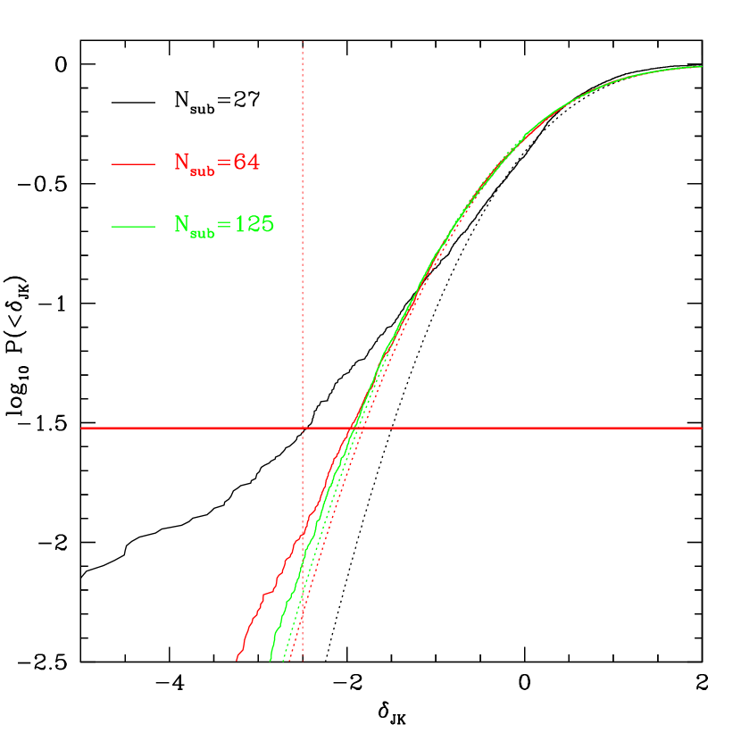
Figure 5: The probability of finding a JK ensemble fluctuation, $\delta_{\rm JK}$, below some value for the distribution of clustering measurements from an ensemble of SDSS mocks made from N-body simulations (see Section 5) for three values of ${\rm N_{\rm sub}}$(solid lines). The $\delta_{\rm JK}$ distribution is estimated here for $\xi(s)$ with ${\rm N_{\rm sub}}$=27, 64 and 125 (black, red and green respectively) over the range $12-14{\,h^{-1}\,{\rm Mpc}}$. The corresponding Gaussian distributions (same colours, but dotted lines) have the same median value and a variance which encloses 68% of the simulation measurements. The JK ensemble fluctuation for small number of JK zones (${\rm N_{\rm sub}}$=27) present a non negligible non-Gaussian tail, highlighting the importance of using N-body simulations to estimate its cumulative probability distribution function, while for larger ${\rm N_{\rm sub}}$ values the distribution can be well approximated by a Gaussian.

2.5 Clustering estimators

In this paper we consider the spherically averaged 2-pt correlation function, $\xi(s)$, and the reduced 3-point correlation function, Q${}_{3}(\alpha)$. The clustering estimators used are described in detail in Norberg et al. (2009) and Gaztañaga et al. (2005), for $\xi(s)$ and Q${}_{3}(\alpha)$ respectively.

In the case of $\xi(s)$, we count all pairs out to a maximum separation in redshift space of $60{\,h^{-1}\,{\rm Mpc}}$. For Q${}_{3}(\alpha)$ we consider triplets in which one side of the triangle is $8{\,h^{-1}\,{\rm Mpc}}$ and the other is $16{\,h^{-1}\,{\rm Mpc}}$, with an opening angle of $\alpha$ between these two sides. This is one of the many configurations considered in Gaztañaga et al. (2005) (see their Fig. 1 for an illustration of the triplet). We have focused on a minimum of $8{\,h^{-1}\,{\rm Mpc}}$ scales for SDSS (as opposed to $6{\,h^{-1}\,{\rm Mpc}}$ in 2dFGRS) because the larger SDSS volume makes it possible to explore larger (weakly non-linear) scales. We follow the implementation of the Jackknife method outlined in Norberg et al. (2009), and briefly summarized in subsection 2.3.

We estimate $\xi(s)$ and Q${}_{3}(\alpha)$ for all of the volume limited samples listed in Table 1, as well as for the Jackknife resamplings of the different dimension quilts considered in this paper, i.e. mainly N_sub= 25 and 225, but also N_sub= 16, 49, and 100.

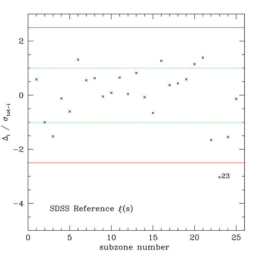
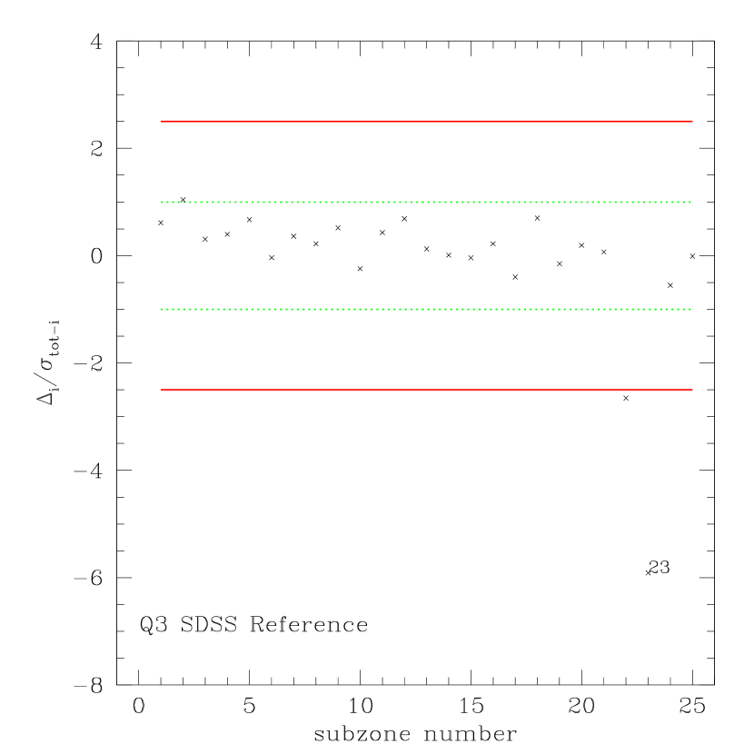
Figure 6: The JK ensemble fluctuation, $\delta_{JK}^{i}$ (as defined in Eq. 6) using pair separations of $12-14{\,h^{-1}\,{\rm Mpc}}$ in $\xi(s)$ (left panel) and triplets separated by similar scales for Q${}_{3}(\alpha)$ (right panel). Each point corresponds to leaving out the zone number plotted on the x-axis. This new statistic is shown in both panels for a ${\rm N_{\rm sub}}$=25 Jackknife quilt, as shown on the left panel of Fig. 2. The fluctuation is plotted using a cross if its value lies within $\pm 3$; otherwise the point is labelled with the zone number that was omitted.

3 Identification of outlying regions

We use a Jackknife technique to identify survey regions which have a big influence on the measured clustering signal. The method consists of comparing clustering measurements from each of the Jackknife resamplings of the data with that obtained from the full dataset. If the measurement from a particular resampling is unusual next to the measurements obtained from the others, then the omitted zone is referred to as an outlying zone. The key here is the definition of “unusual”. The very presence of an outlying zone affects the distribution of measurements from the Jackknife resamplings, with the consequence that simple concepts which apply to Gaussian distributions, such as the mean and variance, need to be redefined. To deal with this we introduce two new statistics to quantify outliers: the JK resampling fluctuation and the JK ensemble fluctuation.

In this section we apply the Jackknife resampling to the ref sample listed in Table 1. We consider the clustering in the other samples listed in Table 1 in Section 4.

3.1 The JK resampling fluctuation

In Fig. 4 we plot the two and three point correlation functions measured from each of the Jackknife resamplings of the ref sample. We show the distribution of these measurements by plotting the scaled quantity $\Delta_{i}$ which is defined as

$$\Delta_{i}=\frac{x_{i}}{x_{\rm full}}-1,$$ (3)

where $x_{i}$ represents a clustering statistic, which in the present paper will be either the two or three point function measured from a JK resampling of the data on omitting zone $i$ and $x_{\rm full}$ indicates the corresponding measurement using the full sample. We call this quantity the JK resampling fluctuation as it quantifies the deviation of the clustering measured on omitting a particular zone from the measurement using the full dataset.

In Fig. 4 we use 25 Jackknife zones. The left panel of Fig. 4 shows the scatter in the two-point correlation function measured from the different resamplings and the right hand panel shows the scatter in Q${}_{3}(\alpha)$. The measurements of $\xi(s)$ and Q${}_{3}(\alpha)$ when omitting zone 23 (which is indicated in Fig. 3) are clear outliers compared to the measurements from the other jackknife resamplings. Both of these measurements lie well outside the variance of the resamplings which is indicated in the plot by the error bars. Note that the variance here corresponds to the range which encloses the central 68% of the JK measurements. Of course, when interpreting this plot it is important to remember that bins of pair separation or opening angle are correlated. Furthermore the measurements from different resamplings are also correlated, as they differ by only 8% in area and hence by the same amount in volume when using 25 Jackknife zones.

3.2 The JK ensemble fluctuation

The fluctuation in the clustering signal on omitting zone 23 is in fact even more significant than suggested by Fig. 4. To demonstrate this we now apply the Jackknife technique to the data in a slightly different way from the standard approach as outlined in Norberg et al (2009). The relative rms error estimated in the standard Jackknife scheme by splitting the data into ${\rm N_{\rm sub}}$ zones is denoted by $\sigma_{\rm tot}$:

$$\sigma_{\rm tot}^{2}={1\over{N_{\rm sub}}}\sum_{i=1}^{N_{\rm sub}}\Delta_{i}^{2},$$ (4)

where $\Delta_{i}$ is the JK fluctuation defined by Eq. 3. We then make a similar error estimate from a new dataset, which is comprised of ${\rm N_{\rm sub}}$$-1$ zones, omitting the $i^{\rm th}$ zone from the set altogether:

$$\sigma_{\rm tot-i}^{2}={1\over{N_{\rm sub}-1}}\sum_{j\neq i}^{N_{\rm sub}-1}\Delta_{j}^{2},$$ (5)

The Jackknife resampling is done in this instance sampling only from the ${\rm N_{\rm sub}}$$-1$ zones, without considering the $i^{\rm th}$ zone at all. The rms error obtained in this way is written as $\sigma_{\rm tot-i}$.

In order to quantify how the scatter in the clustering depends upon which zone is left out, we introduce a new statistic, the JK ensemble fluctuation, $\delta_{JK}^{i}$, defined as:

$$\delta_{JK}^{i}\equiv{\Delta_{i}\over{\sigma_{\rm tot-i}}},$$ (6)

which is just the JK resampling fluctuation for the $i^{\rm th}$ zone normalized to its corresponding rms error, i.e. $\sigma_{\rm tot-i}$.

The probability of finding a particular value of the JK ensemble fluctuation is plotted in Fig. 5 for a distribution which is very similar to that expected for the SDSS data, derived from an ensemble of N-body simulations described in Section 5. In Fig. 5 $\delta_{\rm JK}$ is estimated for $\xi(s)$ over $12-14{\,h^{-1}\,{\rm Mpc}}$, the range of scales most relevant for this paper. For comparison purposes, we plot a Gaussian that has the same median value as that obtained from the simulations and has a variance which corresponds to the range which encloses 68% of the correlation functions measured from the simulations. These distributions describe the expected range of fluctuations in the new JK ensemble fluctuation. For small values of $\delta_{JK}^{i}$ the two distributions are similar, due to the way the Gaussian has been set up. However, they differ appreciably in the tails. In the case of the Gaussian, a value of $\delta_{JK}^{i}<-1.5$ would be obtained 3% of the time, whereas for the distribution from the simulations, we would expect to see such a value in around 8% of cases; the 3% chance in the simulation case corresponds to $\delta_{JK}^{i}<-2.5$. The non-Gaussian nature of the distribution of the JK ensemble fluctuation decreases with the number of JK samples considered, and approaches asymptotically the corresponding Gaussian distribution for $\delta_{JK}$. Therefore for small (large) number of JK samples, one has to consider the non-Gaussian (Gaussian) distribution to estimate the significance level of a given $\delta_{JK}^{i}$.

In Fig. 6 we use the new statistic, $\delta_{JK}^{i}$, defined by Eq. 6, to quantify the significance of the fluctuations in the clustering measurements. The error is calculated using pair separations in the range $12-14{\,h^{-1}\,{\rm Mpc}}$. In the left hand panel we plot JK ensemble fluctuation for $\xi(s)$ on splitting the data into 25 Jackknife zones and in the right we show the corresponding result for Q${}_{3}(\alpha)$, sampling similar scales. Fig. 6 (left-hand panel) shows that if the Jackknife zones were truly independent, then the fluctuation in the rms error on leaving out zone 23 corresponds to $\delta_{JK}^{i}<-3$, which, according to Fig. 5, should occur around 1.6% of the time. For a Gaussian distribution, this large value of $\delta_{JK}^{i}$ is even less likely. We note that this probability comes from the fraction of JK regions from an ensemble of simulations that have $\delta_{\rm JK}<-3$, as $\delta_{\rm JK}$ is estimated for each JK region. In other words, the constraint is on the probability of a JK region being this (or more) extreme and not on the probability that a survey contains such an extreme region. From the simulations we infer that $\sim 50$ percent of SDSS ref like volumes would contain one or more JK regions with $\delta_{\rm JK}<-3$. For Q${}_{3}(\alpha)$ (right-hand panel of Fig. 6) the fluctuation in the rms error on leaving out zone 23 corresponds to $\delta_{\rm JK}^{i}\sim-6$, which translates into a probability of less than $\sim 0.4$% (see Fig. 5), assuming the distribution of the JK ensemble fluctuation is the same for $\xi(s)$ and Q${}_{3}(\alpha)$. It should be noted that the $\delta_{\rm JK}$ distribution should be dependent on the statistic considered, as well as on the number of zones considered. In our comparisons we always find that outliers in Q${}_{3}(\alpha)$ tend to correspond to the ones in $\xi(s)$. Hence we assume here that the distribution of $\delta_{\rm JK}$ is similar for the two and three point correlation functions.

For both the two and three point correlation functions, the measurements on omitting zone 23 are significant outliers, not only visually as in Fig. 4 but also statistically when interpreting their $\delta_{JK}$ value (less than $-3$ for both $\xi(s)$ and Q${}_{3}(\alpha)$) in terms of the global $\delta_{JK}$ distribution as extracted from the simulations. It is not surprising to see that the significance level is much larger for the higher order statistic (i.e. Q${}_{3}(\alpha)$), as it is well known that such statistics are much more sensitive to large scale fluctuations than the two point function. We note that zone 22 is also an outlier for the reduced 3-point statistic, albeit to a much lesser extent than zone 23. This is only really noticeable with this new statistic, as in the right hand panel of Fig. 4 the first impression one has is that zones 22 and 23 are both outliers to roughly a similar extent.

Fig. 7 presents the JK ensemble fluctuation for the ${\rm N_{\rm sub}}$=225 quilt. Zones 187 and 217 to 220 stand out as much as zone 23 did for the ${\rm N_{\rm sub}}$=25 quilt. These zones from the 225 Jackknife quilt are mostly co-spatial and overlap mainly with zones 22 and 23 (and a small amount with zone 24) from the 25 Jackknife quilt, as shown more explicitly in Fig. 3. Together they map out the central parts of the SDSS great wall (Gott et al. 2005), a feature uncovered partially in the earlier 2dFGRS analysis of Baugh et al. (2004). Out of the seven outliers in the 225 Jackknife quilt, five belong to this structure.

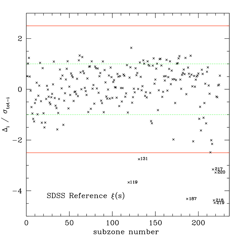
Figure 7: The same plot as in the left panel of Fig. 6, but for ${\rm N_{\rm sub}}$=225, i.e. for the 15x15 Jackknife quilt, as shown in the right panel of Fig. 2. For clarity, crosses have been omitted whenever $|\delta_{\rm JK}|>2.5$. There are 7 zones which present significant deviations from the expectation in the JK ensemble fluctuation statistic (as defined in Eq. 6) using pair separations of $12-14{\,h^{-1}\,{\rm Mpc}}$. For this large ${\rm N_{\rm sub}}$, the $|\delta_{\rm JK}|>2.5$ threshold corresponds to a 2.5-$\sigma$ level, implying that the Gaussian expectation for the number of outliers is just $\sim 1.4\pm 1.2$, significantly lower than the number of observed outliers.

3.3 Blind search and number of JK

The variant on the Jackknife technique we have described in this section is an objective way to find unusual structures in the galaxy distribution. The Jackknife zones provide a blind test to detect superstructures based on uncovering outliers in clustering measurements, although it is unlikely that this method would be the preferred one for actually detecting superstructures. It is certainly more valuable as test of the homogeneity of the JK subsampling chosen. Furthermore, we have introduced a statistic which allows us to quantify the significance of the outliers. Another feature of this approach is that it can be used to suggest the appropriate size of Jackknife zone to use in error estimation. If, for example, we find that several adjacent zones give outlying clustering results, as is the case for the 225 Jackknife quilt above, then the analysis should be repeated with larger zones. In this way, either the outliers disappear or the unusual clustering is restricted to one zone, as we found for the 25 quilt Jackknife. With one outlier zone, one could then present the clustering analysis both with and without this zone to show its impact on the results (as was done in our earlier higher-order clustering analyses of the 2dFGRS, e.g. Baugh et al. 2004; Croton et al. 2004, 2007; Gaztañaga et al. 2005). Similarly, Zehavi et al. (2005, 2011) presented SDSS results for a full M^∗ galaxy sample and for a sample with a redshift limit designed to exclude the Sloan Great Wall.

3.4 Impact on errors

Another consequence of the analysis in this section is the impact of zones containing unusual structures on the error estimated using the Jackknife method. Fig. 4 shows that the Jackknife resampling which produces an outlying cluster statistic can lead to a over estimate of the variance. The blue errorbars in Fig. 4 show the variance estimated using all of the Jackknife resamplings, including the outlier. The red errorbars show the variance estimated from a Jackknife resampling of 24 zones in the 25 patch quilt, leaving out zone 23 altogether. For the two point function, there is a modest reduction in the variance on leaving out the zone containing the superstructure, but more importantly there is a significant uncertainty in the corresponding Jackknife covariance matrix when one sample is the source of most of the variance. This becomes clear in Fig. 6 for both $\xi(s)$ and Q${}_{3}(\alpha)$, where one notices a systematic bias in the scatter in the JK ensemble fluctuation. If all samples were equally important for the variance, this new statistic would be distributed symmetrically around the expectation value. This is not the case for either of the clustering statistics considered here.

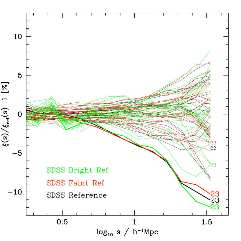
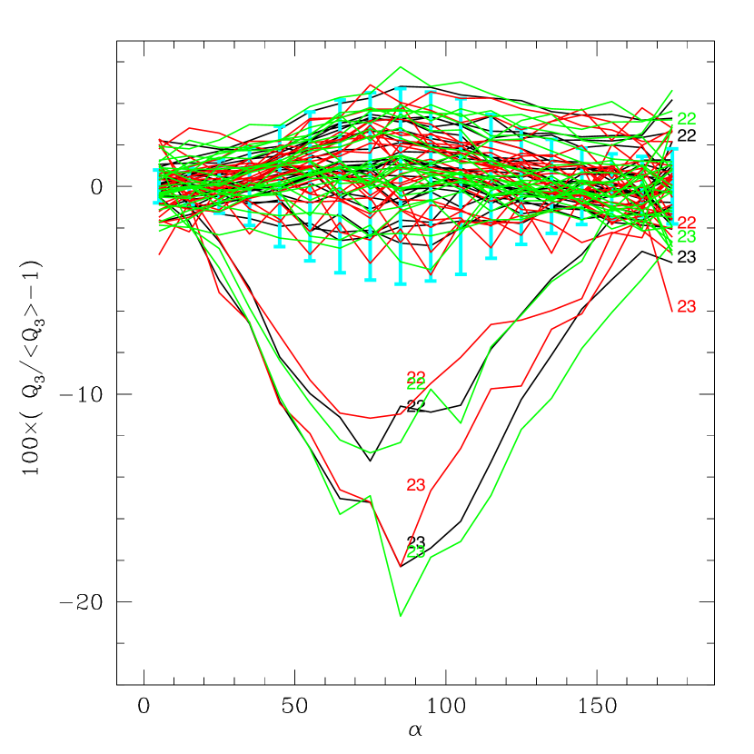
Figure 8: Clustering statistics measured using Jackknife resamplings of galaxies from the same volume, using the ref sample (black), the bright-ref (green) and faint-ref (red). The left-hand panel shows $\xi(s)$ and the right-hand panel Q${}_{3}(\alpha)$. The most significantly outlying clustering statistics are labelled by the omitted zone number (for clarity we place labels both on the center and on the right of each line for $Q_{3}$). The errorbars correspond to the rms clustering error from the Jackknife resamplings of the ref sample.

4 The influence of superstructures

Once we have identified a superstructure using the Jackknife approach set out in the previous section, we can study its influence on the clustering measured from other volume limited samples drawn from the survey. Croton et al. (2005) found that the 2dFGRS superstructures had an impact only on the M^∗ volume limited sample, with Zehavi et al. (2005) reaching almost the same conclusion from their SDSS analysis. In the case of the sample one magnitude brighter than M^∗, the clustering measurements did not show any unusual features, even though the superstructure was also included within the volume. Two things change when moving from the M^∗ volume limited sample to a sample that is one magnitude brighter: the volume of the sample increases and the way in which structures are represented changes. Importantly, the number of galaxies tracing the superstructure is different between the two volume limited samples, and so the contrast of the superstructure will also be different. Also, a larger volume could result in other superstructures being included, diluting the impact of any one structure on the measured clustering.

In an attempt to disentangle and understand these effects (namely, the increase in the volume used to measure clustering and the representation of structures with different numbers of galaxies) we compare clustering measurements in a range of volume limited samples (which are listed in Table 1). All our comparisons use relative clustering statistics for a given sample, allowing us to properly compare different galaxies without the need to model tracer dependent biases, such as luminosity or colour dependent clustering.

First, we look at different tracers within the same volume, to isolate the impact of the sampling of the superstructure or its contrast relative to the other structures within the volume. In Fig. 8, we compare the clustering measured from Jackknife resamplings of the three samples: the ref (one magnitude bin centred on M^∗), the bright-ref (the half magnitude bin brighter than M^∗) and faint-ref (the half magnitude bin fainter than M^∗) samples. These galaxy samples are constrained to cover approximately the same volume and hence are subject to the same underlying density fluctuations. The only difference between them is the number of galaxies which populate the structures within the volume. Fig. 8 shows that the identity of the outlying zone is not sensitive to which galaxies trace out the superstructure within the same volume. The left hand panel of Fig. 8 shows that zone number 23 from the 5x5 Jackknife quilt is a clear outlier for all three samples. The right hand panel of Fig. 8 shows the same comparison between samples for Q${}_{3}(\alpha)$. For this statistic, the omission of two zones, either number 22 or 23, leads to measurements which stand out for all three samples. Hence, the influence of the superstructure is not affected by the number of galaxies used to trace it within a fixed volume, nor by the tracer (to within the limitation of the comparison done here, with galaxies spanning just one magnitude in brightness).

To put our conclusions on a quantitative footing, we show in Fig. 9 the corresponding JK ensemble fluctuation of $\xi(s)$ for the three samples discussed in Fig. 8. As expected, the JK ensemble fluctuation computed for $\xi(s)$ is virtually indistinguishable for the three samples extracted from the same M^∗ volume. Very similar results are found for $Q_{3}$.

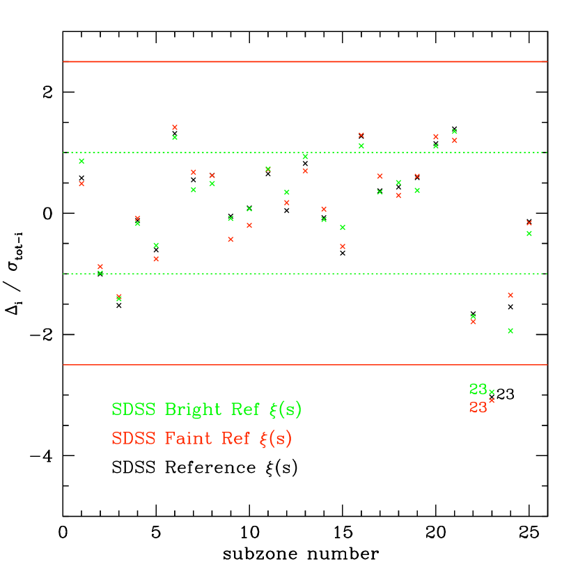
Figure 9: The JK ensemble fluctuation for $\xi(s)$ measured from the ref (black), faint-ref (red) and bright-ref (green) volume limited samples for ${\rm N_{\rm sub}}$= 25.

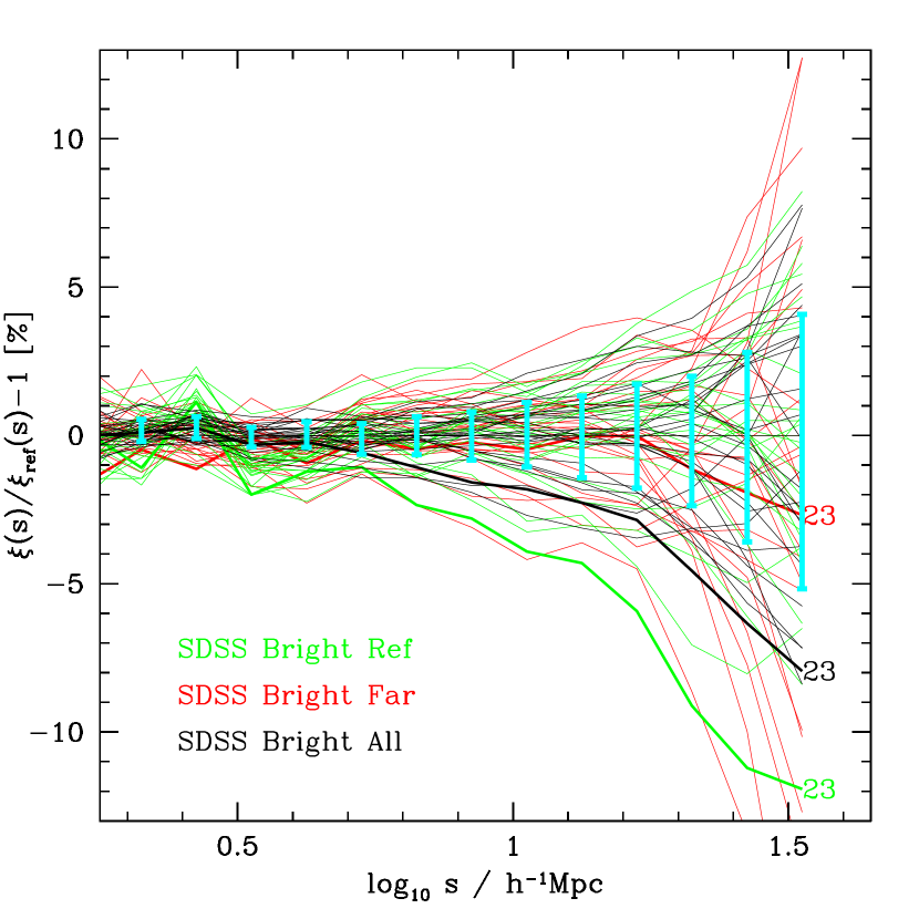
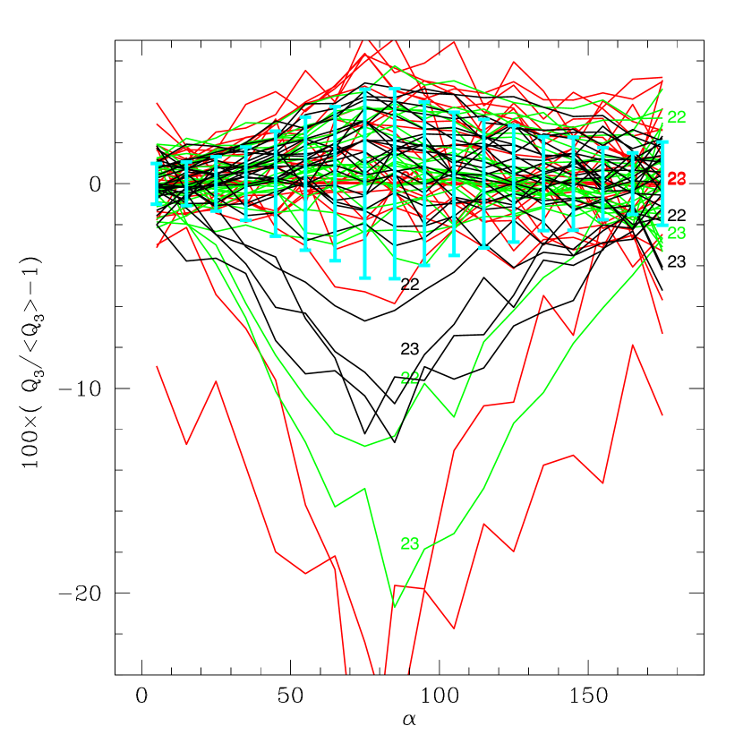
Figure 10: Clustering statistics measured using Jackknife resamplings of bright galaxies from the bright-all (black), bright-far (red) and bright-ref (green) samples (see Table 1). The left-hand panel shows $\xi(s)$ and the right-hand panel shows Q${}_{3}(\alpha)$. Outlying correlation functions that were identified in the ref sample are labelled by the omitted zone number. The errorbars correspond to the rms error from the Jackknife resamplings of the bright-all sample.

The second test we carry out is to compare clustering measurements made from different volumes. Here we consider bright galaxies (i.e. the half magnitude bin brighter than M^∗) as this allows us to cover a wider redshift interval. Again we compare results obtained from three of the samples listed in Table 1: the bright-all, the bright-ref (the low redshift half of bright-all) and the bright-far (the high redshift half of bright-all) samples. The results for the clustering statistics of the Jackknife resamplings of these galaxy samples are shown in Fig. 10. We have labelled the zones which were identified as outliers in the ref sample on Fig. 10. Leaving out zone 23 produces an outlier in the measurements made using the bright-ref sample, as we observed in Fig. 8 already. For the bright-all and bright-far samples, zone 23 is no longer an outlier. The removal of other Jackknife zones leads to larger changes in the measured correlation function. However, the outliers in these cases are not as dramatic as they were in the case of the ref sample. The right-hand panel of Fig. 10 shows the same statistic for Q${}_{3}(\alpha)$. For the bright-ref and bright-all samples, zone numbers 22 and 23 are outliers, but again here not as dramatic in bright-far sample. A different zone is an outlier for the bright-far sample, as happened for $\xi(s)$.

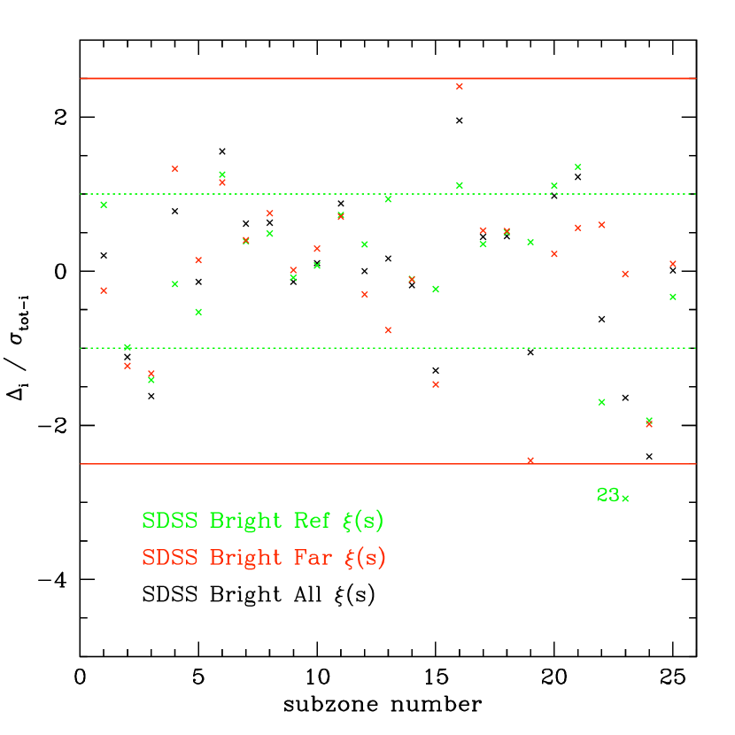
Figure 11: The JK ensemble statistic for $\xi$ measured using ${\rm N_{\rm sub}}$=25 for the bright-all, bright-far, bright-ref volume limited samples, plotted in black, red and green respectively. As expected, samples with the same type of galaxies but covering different volumes do not have the same JK ensemble fluctuation but more importantly, the larger the volume the less influential any given zone becomes.

Again, we quantify the above conclusions by computing the JK ensemble fluctuation. We show in Fig. 11 the JK ensemble fluctuation of $\xi(s)$ for the three samples discussed in Fig. 10. As expected, zone 23 is only an outlier in terms of this statistic for the ref sample, while in the two other samples, i.e. bright-all and bright-far, the JK ensemble fluctuation statistic for $\xi(s)$ points to less extreme results for the zones, with bright-all being the most “uniform” of the three samples considered: this is due to its volume being twice that of the two other samples. Finally the most extreme zone of bright-all is a zone which in both bright-ref and bright-far corresponds to $\delta_{JK}^{i}\sim-2.0$ in the JK ensemble fluctuation statistic. Very similar results are found for $Q_{3}$.

As the zones we use are defined in angle, they cover a wide baseline in redshift and many individual structures could contribute to what we are calling a superstructure. Also, by increasing the volume, other structures could be sampled which could have a similar impact on the clustering signal. The comparison of the scatter of the Jackknife resamplings in the bright sampling volume shows that the omission of different zones can lead to outlying clustering measurements. However, the departure for a given sub-volume from the rest of population seems to become less significant the larger the volume.

4.1 JK ensemble: a practical recipe

With the JK ensemble fluctuation statistic one can assess whether a sample has been split into the right number of sub-zones for a Jackknife error analysis to be valid, as opposed to split into too many small JK regions. The way to proceed is by taking the following steps:

1. the size and number of JK regions should be such that there is no “apparent clustering” in the $\delta_{\rm JK}$ statistic of neighbouring zones (i.e. neighbouring zones should have $\delta_{\rm JK}$ values which are independent from eachother).

2. no JK region should present too extreme a value for $\delta_{\rm JK}$ statistic compared to the others, i.e. the associated probability of its occurence (as derived from the $\delta_{\rm JK}$ distribution as shown in Fig. 5 for $\xi(s)$ with three values of ${\rm N_{\rm sub}}$) should not be significantly at odds with the probability of such an event actually happening (which for large ${\rm N_{\rm sub}}$ values can be modelled by a Gaussian process with ${\rm N_{\rm sub}}$ elements).

3. The probability threshold recommended by the present work is $\sim 3$% (i.e. about 2-$\sigma$ if Gaussian distributed). This corresponds to $\delta_{\rm JK}=-2.5$ for $\xi(s)$ with ${\rm N_{\rm sub}}$=27, and $\delta_{\rm JK}\simeq-2$ for larger ${\rm N_{\rm sub}}$ values (according to Fig. 5).

It is not always possible to find an appropriate number of JK subsamples into which the survey should be split which satisfies both conditions (a) and (b), unless one is reduced to use far too few subsamples from which a statistical inference can be made. In the limit ${\rm N_{\rm sub}}$=1, both conditions are automatically satisfied, but no errors can be inferred. For example in our analysis of the SDSS M^∗ sample (ref sample in Table 1), ${\rm N_{\rm sub}}$=25 is not appropriate, but at least better than ${\rm N_{\rm sub}}$=225. The JK ensemble fluctuation statistic provides a quantitative measure of the limitation of the error analysis and an indication of the need to proceed with further checks before statistically interpreting the results. For example, do the outliers agree with the expectations from simulations? In summary, when conditions (a) and (b) cannot be satisfied, we should use statistical inference with greater care than simply assuming that a comprehensive (but inappropriate) error analysis has solved the problem entierly.

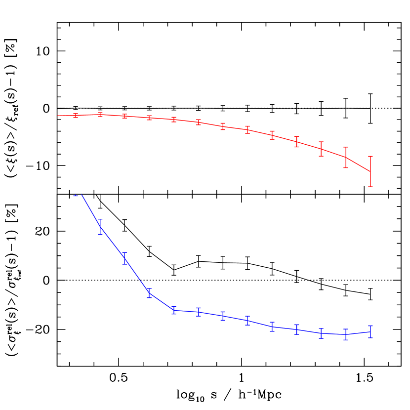
Figure 12: Top: The percentage deviation in the 2-pt correlation function over the N-body ensemble of realisations. The mean result for all the JK resamplings is shown in black, while the red curve shows the result of considering only the outlying regions, which are defined as those for which $|\delta_{\rm JK}|>2.5$. Errorbars show the error on the mean. Bottom: The percentage difference in the relative error on the 2-pt correlation function compared to the N-body ensemble of realisations. As in the top panel, the black line shows the mean result for the ensemble of JK resamplings, while the blue curve presents the result of estimating the 2-pt clustering error after discarding the outlying JK region from the error analysis, with errorbars showing the error on the mean. The top panel shows that discarding the outlying regions affects systematically the overall clustering amplitude on the scales of interest (from $\sim 2$ to $\sim 10$ per cent between 3 and 30${\,h^{-1}\,{\rm Mpc}}$). The bottom panel shows that ignoring the outliers just for the error analysis introduces a systematic underestimate of $\sim 10$ to $\sim 20$ per cent on those same scales, while the ensemble of JK resamplings reproduces fairly accurately the results from the ensemble of N-body simulations (to within a few percent). Further details are given in §4.2.

4.2 Should one ignore the outliers in the analysis?

An interesting question to ask is: ”Is it better to ignore an outlying region altogether when estimating a clustering statistic and its associated error?” From a Bayesian point of view, such a “massaging” of the data set is clearly unattractive, but because it has regularly happened in the past (e.g. Zehavi et al. 2002, 2005, 2011 for 2-pt clustering statistics of SDSS M^∗ samples) we investigate here what consequences this can have.

A proper analysis to answer the above question would require the recalculation of all clustering statistics and discarding from the start all JK regions identified as outliers. Indeed, the way our JK ensemble fluctuation works is such that if JK region $i$ is an outlier, then all other JK estimates contain region $i$. Hence discarding JK region $i$ requires the re-estimation of the clustering signal using only the remaining ${\rm N_{\rm sub}}$-1 JK regions. Such a calculation is unfortunately beyond the scope of this paper, so instead we propose the following two tests:

• the mean clustering signal from outlying regions should be comparable to the mean clustering signal from the ensemble of simulations. If not, then ignoring the outlying regions will influence the overall amplitude of the clustering signal, which clearly is unwanted.

• if one cannot ignore the outlying JK regions in the estimate of the clustering statistic, is it valid to ignore them in the error estimate of the clustering signal? The point here is to understand whether excessive fluctuation due to a “single” region is better discarded in the error analysis.

These two tests are minimal conditions to be satisfied for discarding outlying regions from the analysis, where outlying region is defined here by $|\delta_{\rm JK}|>2.5$, appropriate for a $\sim 2$-$\sigma$ cut for ${\rm N_{\rm sub}}$=27.

To answer test (a), the top panel of Fig. 12 displays the relative effect on the 2-point clustering signal of discarding the outlying regions (red) or using the ensemble of JK resamlpings (black). In both cases the results are compared to the clustering signal from the ensemble of N-body simulations ($\xi_{ref}(s)$, with error $\sigma_{\xi_{ref}}(s)$). The errorbars show the error on the mean, which is the relevant quantity for the present analysis as we are interested in the mean trend and any deviations from its expected value (as shown by the dotted horizontal line). To avoid new estimates to be calculated, the red curve shows the results from averaging the clustering signal in all the outlying regions, selected from each simulation via the condition $|\delta_{\rm JK}|>2.5$. We point out that we had to ignore volumes with two or more outliers ($\sim 10$ per cent of the volumes), as in those cases the clustering signal of an outlying JK region is not necessarily representative of the clustering of the volume with all outlying regions removed. The top panel of Fig. 12 clearly shows that the outlying JK regions have a systematically different clustering signal from the simulation ensemble, hence ignoring them in any clustering analysis would result in systematically low clustering amplitudes. We additionally note that there is scale dependence in this bias, changing from $\sim 2$ to $\sim 10$ per cent between 3 and 30 ${\,h^{-1}\,{\rm Mpc}}$.

To answer test (b), the bottom panel of Fig. 12 displays the percentage difference in the relative error on the 2-point clustering signal of discarding the outlying regions (blue) or using the ensemble of JK resamplings (black). In both cases the results are compared to the relative clustering error from the ensemble of N-body simulations, i.e. $\sigma_{\xi_{ref}}^{rel}(s)$. As for the top panel, the errorbars indicate the error on the mean. Since test (a) showed that it is incorrect to ignore the outlying JK region for the estimate of $\xi(s)$ and to avoid calculating new clustering estimates, the blue curve shows in fact the results from averaging the relative error on $\xi(s)$ ignoring the contribution from all the outlying regions, selected from each simulation via the condition $|\delta_{\rm JK}|>2.5$. Yet again, only simulation volumes with one single outlying region were considered, as only for these volumes can we relate the excess clustering to one JK region (which does not require any reestimation of the clustering statistics). The bottom panel of Fig. 12 shows that, while the relative error from the ensemble of JK resamplings is within a few per cent of the relative error from the simulation ensemble, the relative error estimated from ignoring the outlying regions is underestimated by typically 15 to 20 per cent on scales above $\sim 5{\,h^{-1}\,{\rm Mpc}}$. It is worth noting that the error on scales smaller than a few ${\,h^{-1}\,{\rm Mpc}}$ is, as already noted in Norberg et al. (2009), overestimated by a significant amount when using JK resamplings compared to the simulation ensemble.

Hence using our series of N-body simulations we have shown in this section that not including the outlying JK region in the estimate of the clustering statistic and its errors significantly affects the results and hence should be avoided.

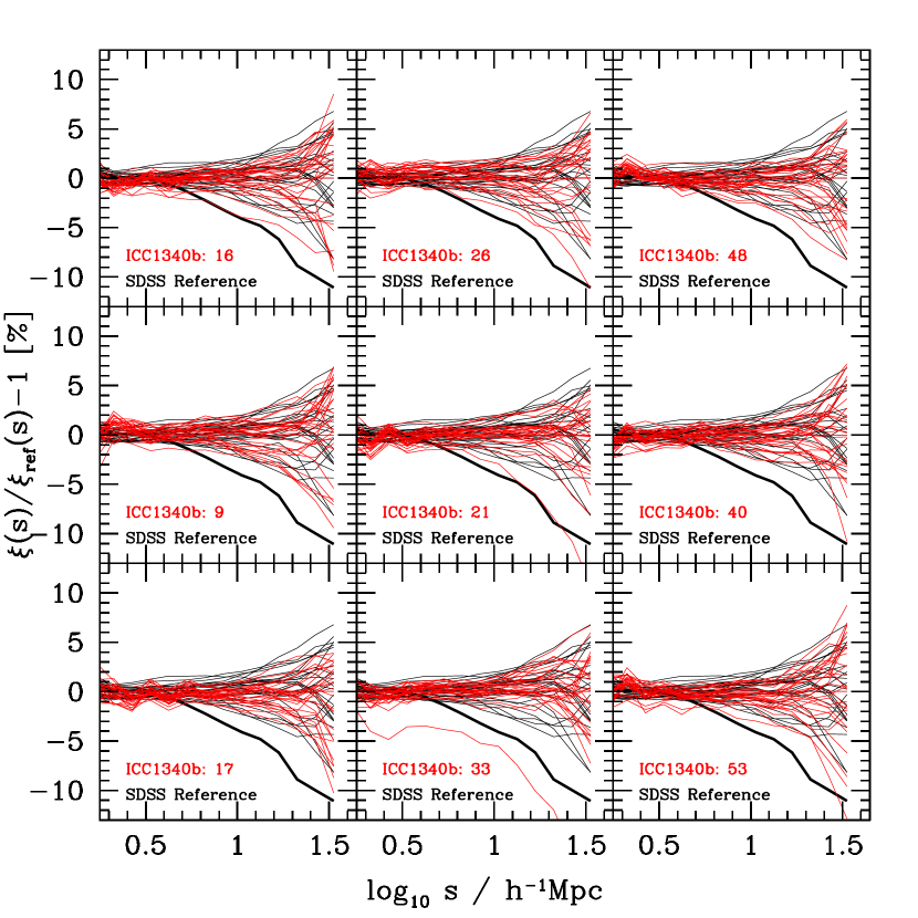
Figure 13: The JK resampling fluctuation for the two-point correlation function in nine (one per panel) randomly chosen L-BASICC $\Lambda$CDM simulations that are all statistically similar and from which a volume comparable to a M^∗ SDSS sample has been extracted (red lines). The equivalent statistic for the SDSS data is shown using black lines and is reproduced in each panel. The thick black line shows the clustering measured on omitting zone 23.

5 Is the SDSS M^∗ sample compatible with $\Lambda$CDM?

Having identified an unusual overdensity of M^∗ galaxies in the SDSS, it is natural to ask if such a structure is expected in the $\Lambda$CDM cosmology. We address this question using a suite of large volume N-body simulations by Angulo et al. (2008). The same calculations were used in the evaluation of internal error estimation schemes by Norberg et al. (2009).

The L-BASICC simulation ensemble of Angulo et al. (2008) comprises 50 moderate resolution runs, each representing the matter distribution using $448^{3}$ particles of mass $1.85\times 10^{12}\,h^{-1}\,M_{\odot}$ in a box of side $1340h^{-1}$Mpc. Each L-BASICC simulation was evolved from a different realization of a Gaussian density field set up at $z=63$, using the following cosmological parameters $\Omega_{\rm M}=0.25$, $\Omega_{\Lambda}=0.75$, $\sigma_{8}=0.9$, $n=1$, $w=-1$ and $h=H_{0}/(100\,{\rm km\,s}^{-1}{\rm Mpc}^{-1})=0.73$. The combination of a large number of independent realizations and the huge simulation volume make the L-BASICC ensemble ideal for searching for unusual structures (see also Yaryura, Baugh & Angulo 2010).

Following the method set out in Norberg et al. (2009), we extract from each simulation cube two cubical sub-volumes of $380~{}{\,h^{-1}\,{\rm Mpc}}$ on a side, which are separated by at least $\sim 500~{}{\,h^{-1}\,{\rm Mpc}}$. These pairs of volumes are correlated because they come from the same simulation box. However, in practice, because of the wide separation of the subvolumes and the low amplitude of the power at these wavelengths, we can treat them as being independent. Hence, with this procedure we construct 100 mock catalogues each of which is fully independent of 98 of the others (as these come from different simulation boxes) and is essentially independent of the other subvolume taken from the same simulation.

The redshift space distortion of clustering is not modelled using the distant observer approximation within the extracted region. Instead we place the observer at the centre of the simulation volume and extract a region that is at a distance comparable to the SDSS M^∗ sample, i.e. $\sim 300{\,h^{-1}\,{\rm Mpc}}$ away. The cubical region that we extract is somewhat bigger than the SDSS M^∗ sample. This is to provide a spatial buffer, as peculiar velocities can displace particles in either direction along the line of sight, and particles can be moved into as well as out of the volume of interest. Finally, we randomly dilute the number of dark matter particles in each data set to match the number density of the M^∗ galaxy sample of $3.7\times 10^{-3}~{}{\,h^{-3}\,{\rm Mpc^{3}}}$, which mimics the discreteness or shot noise level in the SDSS M^∗ volume limited sample. Following Norberg et al. (2009), we do not attempt to model a particular galaxy sample and survey geometry in detail, but simply to cover a comparable volume with the same number density of objects. Our aim here is to make a generic comparison: are enough large structures expected in the $\Lambda$CDM cosmology to account for the outliers we have seen in 1/25^th of a volume limited M^∗ SDSS galaxy sample?

We repeat the Jackknife resampling analysis we carried out earlier for the SDSS data samples, but for the L-BASICC dark matter catalogues and present the 2-point clustering estimates in Fig. 13. Each panel shows results for a different subvolume from the ensemble (in red with the subsample number indicated in the panel legend) and the corresponding result for the SDSS ref sample (in black and replicated in all panels). Each line corresponds to the fluctuation of $\xi(s)$ measured from one of the N_sub Jackknife resamplings around the measurement from the corresponding full volume limited sample.

The L-BASICC regions we analyze have a volume equal to that of the bright-all sample, which is twice the size of the ref sample, so we expect the scatter in the Jackknife resamplings for the simulations to be smaller than for the ref sample. We found a similar result in Fig. 10 with the scatter from the bright-all sample being systematically smaller than either of its two components, i.e. bright-far and bright-far.

Mainly for this reason and for slight mismatches between the simulation and the SDSS data (see Norberg et al. 2009 for a detailed discussion), the scatter measured in the simulation results should be considered as a lower limit compared to that displayed by the SDSS data in the ref sample, or better matched to the bright-all sample (based on simple volume arguments). The main conclusion we can draw from Fig. 13 is that outliers comparable to or even more extreme than that produced by zone 23 in the data are reasonably common in the $\Lambda$CDM cosmology. In approximately one third of the randomly chosen cases, the scatter in the simulation Jackknife resamplings is comparable to what is seen in our reference volume limited sample. Hence the structure in zone 23 does not present a problem for $\Lambda$CDM .

6 Superstructures in 2dFGRS & SDSS

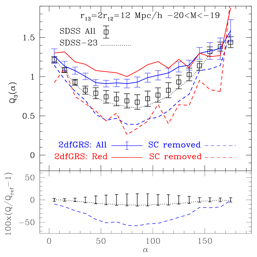
Figure 14: Comparison of Q${}_{3}(\alpha)$ estimates from the 2dFGRS (blue continuous line with errorbars) and SDSS (open squares with errorbars). SDSS errorbars are from the $N_{\rm sub}=25$ JK subsamples. 2dFGRS errors are from the dispersion of 22 galaxy mocks that match 2dFGRS 2-point correlations (see Gaztañaga et al. 2005 for details). The dashed blue line corresponds to the 2dFGRS measurement after removing the 2 largest superclusters. The dotted line corresponds to result from the SDSS after leaving out JK subsample 23 (ie all minus outlier subregion 23 in Fig.3). Red lines show the corresponding results from the 2dFGRS red selected sample, which ought to provide a better comparison with the r-band SDSS selected galaxies. Errorbars in the bottom panel show the relative JK rms fluctuations in SDSS (same as in Fig. 4 but scaled by usual JK factor $\sqrt{N_{\rm sub}}=5$). The dotted line corresponds to results after leaving out SDSS JK subsample 23. The blue dashed line shows the relative fluctuation for the 2dFGRS sample after excluding the superstructures.

Previous studies which estimated the higher-order clustering statistics from the 2dFGRS (e.g. Baugh et al. 2004; Croton et al. 2004, 2007; Gaztañaga et al. 2005) and SDSS surveys (e.g. Nichol et al. 2006; Mcbride et al. 2011) found that the presence of one or two superstructures had a strong influence on the interpretation of the measurements for their M^∗ samples, which are all similar in their definitions to the one considered here, covering roughly the same redshift range, i.e. $0.05\lesssim z\lesssim 0.11$ and sampling mostly M^∗ galaxies. In some work, clustering statistics were presented both for full samples and for samples from which the volume containing the superstructure had been cut out, referred to as the “with” and “without” supercluster results. This practice was merely intended to illustrate the impact of these structures on the measurements, rather than to advocate one or the other as being the definitive or correct answer. An example of this practice is shown for the 2dFGRS in Fig. 14, which shows the “with” and “without” measurements of the 3-point function for the M^∗ volume limited sample, as first presented in Gaztañaga et al. (2005). At that time, because of the substantial difference between these two measurements, the M^∗ sample results were considered unreliable. Therefore the analysis and interpretation focused mostly on larger volume limited samples, corresponding to brighter galaxies. Due to a combination of increased volume and the way in which brighter galaxies sample or weight structures (compared to M^∗ galaxies) these volume limited samples seemed to be less affected by any particular superstructure.

There is one subtle, but important difference between these previous analyses and the one presented in this paper. Here an objective, blind approach is taken, while in the earlier works, a bespoke supercluster mask was constructed, starting from the location of high peaks in the 3-D density field and then masking all galaxies within a radius of $25{\,h^{-1}\,{\rm Mpc}}$ from the centre of the peak (see Baugh et al. 2004 and Croton et al. 2004 for details). This method actually results in a more significant difference between the measurements “with” and “without” the superclusters. It is therefore natural to revisit these results and compare them with the more objective method considered here.

In Fig. 14 we show a comparison between Q${}_{3}(\alpha)$ estimated from the 2dFGRS and SDSS M^∗ samples. The 2dFGRS clustering estimates are from Gaztañaga et al. (2005), with two sets of measurements plotted: the with superclusters measurement (continuous lines) and the without superclusters measurement (dashed lines). The SDSS DR7 measurements from the ref sample (squares with errorbars) are new and fall consistently between the results from the 2dFGRS analysis. It is reassuring to see how clustering measurements for 3-point statistics are reproducible: they come from different parts of the sky, are obtained using different telescopes/cameras and, most importantly, are based on slightly different galaxy selections. To attempt to remove the difference in selection between the 2dFGRS and SDSS samples, we also show the results for the 2dFGRS, both with and without superclusters, for a red selected subsample (see Gaztañaga et al. 2005 for the exact definition of their red selected 2dFGRS M^∗ sample). This should be more comparable to the selection in the SDSS, which is done in the $r-$band. The results are noisier because of the smaller number of galaxies retained, but are similar to the measurements from the full, blue selected 2dFGRS sample.

In the bottom panel of Fig. 14, the dashed (blue) line indicates the relative difference in Q${}_{3}(\alpha)$ (in percent) measured from the 2dFGRS when we compare results with and without the superclusters. The effect seen in the 2dFGRS is much larger than the analogous result in Fig. 4 for the SDSS. The SDSS measurement is characterized by the errorbars in the bottom panel of Fig. 14, scaled by the usual JK factor $\sqrt{N_{\rm sub}}=5$ to show the variance in the full sample (as opposed to the variance in the JK-subsample displayed in Fig. 4). The shift in the measurement of $Q_{3}$ from the SDSS on leaving out the outlier subregion 23 is shown by the dotted line. For the 2dFGRS, removing the supercluster from the clustering analysis produces a change of up to $\sim 50$ per cent in Q${}_{3}(\alpha)$, while the corresponding number for the SDSS using the more objective method of JK resampling introduced here is $\sim 12$ per cent. These differences reflect both that the 2dFGRS is $\sim 5$ times smaller than SDSS and also the different ways in which outlying superstructures are defined in each case. Also note how the SDSS measurement on leaving out the outlier subregion is still within the JK errors while the 2dFGRS measurement without superclusters is outside the errors (which came from an ensemble of 22 mock catalogues).

What have we learnt from this? From our new outlier analysis using Jackknife resampling and for the particular statistics (and scales) we consider, the impact of large scale inhomogeneities in the SDSS M^∗ sample can be as large as $\sim 12\%$ in Q${}_{3}(\alpha)$ on scales of $12-14{\,h^{-1}\,{\rm Mpc}}$. We can and should use this information to test models, both in terms of interpreting a fit to the data and in terms of the outlier probability in realizations of a given model. These outlier probabilities are now significantly better defined than before, as is clear from the bottom panel of Fig. 14 through the difference between the 2dFGRS estimate “with” and “without” superclusters and the statistical Jackknife resampling method. More importantly, as shown in the previous section, we can apply the same objective algorithm (i.e. the Jackknife resampling method) to both data and simulations enabling statistically robust conclusions to be drawn. The previous method applied to the 2dFGRS, based on removing superstructures, is subjective and significantly harder to transfer from data to mocks. It is now clear from the comparison between the 2dFGRS and SDSS results in Fig. 14 that the error bars derived from mock 2dFGRS catalogues did not capture the full variance in that sample. This can be better understood if one accounts for the various limitations of the mocks, i.e. (a) we have only 22 non-overlapping (but still not independent) mocks drawn from the same Hubble Volume simulation (Evrard et al. 2002); (b) the mocks are only constrained to reproduce the two-point 2dFGRS galaxy clustering (Cole et al. 1998); (c) errors on clustering statistics depend directly on their higher order moments (e.g. Bernardeau et al. 2002). This was already noted by Gaztanaga et al. (2005) who considered this sample to be unreliable because of the effect of the superclusters. The situation is different for the SDSS analysis presented here (in Fig. 14) where, despite the presence of the outlier region 23 (i.e. see Fig.3), we can be more confident of the error analysis because we have a systematic way to quantify the impact of outliers.

7 Summary

This paper presents a new method to quantify the robustness of error estimates for clustering statistics. The approach is an extension of the Jackknife technique and uses two new clustering diagnostics to quantify the distribution of clustering measurements from different resamplings: the JK resampling fluctuation (first shown in Fig. 4), and the JK ensemble fluctuation (first shown in Fig. 6). The main features of the method can be summarized as follows:

• The technique provides an objective way of finding large coherent structures. As the Jackknife zones are set up a priori, this is a blind test for the presences of superstructures, based on their impact on the measured clustering statistics. This is an improvement over earlier work in which “unusual” regions were omitted after making the clustering measurements, without any firm guidance as to what volume should be excluded.

• Our approach provides a quantitative way of determining the appropriate size of the Jackknife zones to be used in the error analysis of the clustering signal. It follows these three key ingredients:

  1. the size and number of JK regions should be such that there is no “apparent clustering” in the $\delta_{\rm JK}$ statistic of neighbouring zones (i.e. neighbouring zones should have $\delta_{\rm JK}$ values which are independent from eachother).

  2. no JK region should present too extreme a $\delta_{\rm JK}$ statistic compared to the others, i.e. the associated probability of its occurence (as derived from the $\delta_{\rm JK}$ distribution as shown in Fig. 5 for $\xi(s)$ with three values of ${\rm N_{\rm sub}}$) should not be significantly at odds with the probability of such an event actually happening (which for large ${\rm N_{\rm sub}}$ values can be modelled by a Gaussian process with ${\rm N_{\rm sub}}$ elements).

  3. The probability threshold recommended by the present work is $\sim 3$% (i.e. about 2-$\sigma$ if Gaussian distributed). This corresponds to $\delta_{\rm JK}=-2.5$ for $\xi(s)$ with ${\rm N_{\rm sub}}$=27, and $\delta_{\rm JK}\simeq-2$ for larger ${\rm N_{\rm sub}}$ values (according to Fig. 5).

• The new statistics we have introduced can be used to compare observations to models. As shown in §5, we can check in a straight forward and objective way whether or not simulations produce similar outlying clustering measurements as those seen in the data. Again, this is a significant improvement over the ad-hoc approach of computing the correlation functions “with” and “without” the superstructrures.

• The statistics offer a quantitative way to study the influence of large coherent structures on the measured correlation function, even if the structures dominate the clustering signal. As shown in §6, with these new tools we can quantify how inhomogeneities affect our measurements and the reliability of our error estimates.

In the standard application of the Jackknife method to galaxy surveys, the dataset is divided spatially into zones. Our procedure overcomes one of the long standing problems of Jackknife error estimation: how many zones should the data be split up into? A large number of zones implies a large number of resamplings of the dataset. To improve the stability of the inversion of the covariance martix, it is important to have as large as possible a number of resamplings (e.g. Hartlap et al. 2007). This is a vague concept, as if the Jackknife zones are made too small, the resamplings will be essentially the same, with a very small change in the volume covered. Our approach uses the Jackknife ensemble fluctuation to determine the appropriate number of zones. This statistic allows us to identify the omission of a zone as leading to an outlying clustering measurement. We have argued that such outliers should be due to the structure contained within one Jackknife zone, rather than several contiguous zones. In our illustration using the M^∗ SDSS volume limited sample, this suggested that ${\rm N_{\rm sub}}$=25 is a more robust number of zones to use in the Jackknife method than ${\rm N_{\rm sub}}$=225.

The approach we have set out in this paper, along with the comparison between different error estimation methods presented in Norberg et al. (2009), provides a robust and objective presciption for the estimation of galaxy correlation functions and their associated errors, which can be applied to any type of forthcoming survey, both spectroscopic and photometric.

Appendix A SQL queries

In this appendix we list the SQL queries and data files used to generate the galaxy catalogues and to construct the imaging and spectroscopic completeness masks used in the paper.

A.1 Galaxy Catalogue

The CasJobs SQL query used to generate the input galaxy catalogue from which the spectroscopic galaxy catalogue is derived is:

SELECT ...
INTO ...
FROM PhotoPrimary po
LEFT OUTER JOIN Target t on t.bestObjID = po.objid
LEFT OUTER JOIN SpecObj so on po.specObjID = so.specObjID
where po.primtarget&(64|128|256)!=0 and po.status&(16384)!=0
and t.targetID > 0

This query accounts for galaxies with and without redshifts, but which were intended for spectroscopic targeting. Only galaxies whose redshift satisfies the GAMA (Driver et al. 2009, 2010) selection criteria for a good redshift (see Baldry et al. 2010 for the exact definition) are used in the clustering analysis.

A.2 Imaging and Spectroscopic Mask

To generate the imaging and spectroscopic masks, the following CasJobs SQL query can be used :

SELECT
run,field,raMin,raMax,decMin,decMax,
rerun,camcol,skyVersion
FROM field

together with these two DR7 files:

http://www.sdss.org/dr7/coverage/tsChunk.dr7.best.par

http://www.sdss.org/dr7/coverage/maindr72spectro.par

listing the imaging coverage and the position of the spectroscopic tiles respectively. It is also necessary to include the information about additional “holes” in SDSS DR7 coverage, as listed on

http://www.sdss.org/dr7/coverage/holes.html .

The masks, quilts and galaxy catalogues can be made available upon request by contacting lead author.

References

- [XX XX] Abazajian K.N., et al., 2009, ApJS, 182, 543
- [XX XX] Angulo R.E., Baugh C.M., Frenk C.S., Lacey C.G., 2008, MNRAS, 383, 755
- [Baldry et al. 2010] Baldry I.K., et al., 2010, MNRAS, 404, 86
- [Baugh et al. 1995] Baugh C.M., Gaztañaga E. & Efstathiou G., 1995, MNRAS, 274, 1049
- [Baugh et al. 2004] Baugh C.M., et al., 2004, MNRAS, 351, L44
- [XX XX] Bernardeau F., Colombi S., Gaztañaga E., & Scoccimarro R., 2002, Phys. Rep. 367, 1
- [XX XX] Blanton M.R., et al., 2003, AJ, 125, 2348
- [XX XX] Blanton M.R., et al., 2003, ApJ, 592, 819
- [Cole et al. 1998] Cole S., Hatton S., Weinberg D.H., Frenk C.S., 1998, MNRAS 300, 945
- [Cole et al. 2005] Cole S., et al., 2005, MNRAS 362, 505
- [Colless et al. 2001] Colless M., et al., 2001, MNRAS, 328, 1039
- [Colless et al. 2003] Colless M., et al., 2003, astro-ph/0306581
- [Croft et al. 2004] Croft R.A.C., Dalton G.B. & Efstathiou G., 1999, MNRAS 305, 547
- [Croton et al. 2004] Croton D.J., et al., 2004, MNRAS 352, 1232
- [Croton et al. 2007] Croton D.J., et al., 2007, MNRAS 379, 1562
- [Driver et al. 2009] Driver S.P., et al., 2009, A&G, 50e, 12
- [Driver et al. 2010] Driver S.P., et al., 2011, MNRAS 413, 971
- [Evrard et al. 2002] Evrard A., et al., 2002, ApJ 573, 7
- [Gaztañaga 2005] Gaztañaga E., Norberg P., Baugh C.M., Croton D.J., 2005, MNRAS 364, 620
- [Gott et al. 2005] Gott J.R., et al., 2005, ApJ 624, 463
- [XX XX] Hartlap J., Simon P., Schneider P., 2007, A&A 464, 399
- [XX XX] McBride C.K., Connolly A.J., Gardner J.P., Scranton R., Newman J.A., Scoccimarro R., Zehavi I., Schneider D.P., 2011, ApJ 726, 13
- [XX XX] McBride C.K., Connolly A.J., Gardner J.P., Scranton R., Scoccimarro R., Berlind A.A., Marin F., Schneider D.P., 2011, 2010arXiv1012.3462
- [XX XX] Miller R.G., 1974, Biometrika, 61, 1
- [Nichol et al. 2006] Nichol R.C, et al., 2006, MNRAS 368, 1507
- [XX XX] Norberg P., et al., 2002, MNRAS 332, 827
- [XX XX] Norberg P., et al., 2009, MNRAS 396, 19
- [XX XX] Roche N., Shanks T., Metcalfe N., Fong R., 1993, MNRAS 263, 360
- [XX XX] Roche N., & Eales S.A., 1999, MNRAS 307, 703
- [XX XX] Strauss M.A., et al., 2002, AJ, 124, 1810
- [XX XX] Tucker D.L., et al., 2006, AN, 327,821
- [XX XX] Tukey J.W., 1958, Ann. Math. Stat. 29, 614
- [XX XX] Yaryura Y., Baugh C.M., & Angulo R., 2011, MNRAS 413, 1311
- [York et al. 2000] York D.G., et al., AJ, 120, 1579, 2000
- [XX XX] Zehavi I., et al., 2002, ApJ 571, 172
- [XX XX] Zehavi I., et al., 2004, ApJ 608, 16
- [XX XX] Zehavi I., et al., 2005, ApJ 630, 1
- [XX XX] Zehavi I., et al., 2011, 2010arXiv1005.2413