Second-order quasiparticle interaction in nuclear matter
with chiral two-nucleon interactions

Abstract

We employ Landau’s theory of normal Fermi liquids to study the quasiparticle interaction in nuclear matter in the vicinity of saturation density. Realistic low-momentum nucleon-nucleon interactions evolved from the Idaho N³LO chiral two-body potential are used as input potentials. We derive for the first time exact results for the central part of the quasiparticle interaction computed to second order in perturbation theory, from which we extract the $L=0$ and $L=1$ Landau parameters as well as some relevant bulk equilibrium properties of nuclear matter. The accuracy of the intricate numerical calculations is tested with analytical results derived for scalar-isoscalar boson exchange and (modified) pion exchange at second order. The explicit dependence of the Fermi liquid parameters on the low-momentum cutoff scale is studied, which provides important insight into the scale variation of phase-shift equivalent two-body potentials. This leads naturally to explore the role that three-nucleon forces must play in the effective interaction between two quasiparticles.

I Introduction

Describing the properties of infinite nuclear matter has long been an important benchmark for realistic models of the nuclear force and the applied many-body methods. Recent calculations fritsch05 ; bogner05 ; siu09 ; hebeler11 have shown that the (Goldstone) linked-diagram expansion (up to at least second order) can provide an adequate description of the zero-temperature equation of state when realistic two-nucleon and three-nucleon forces are employed. In the present work we study nuclear matter from the perspective of Landau’s Fermi liquid theory landau57 ; migdal1 ; migdal2 ; baym , which is a framework for describing excitations of strongly-interacting normal Fermi systems in terms of weakly-interacting quasiparticles. Although the complete description of the interacting many-body ground state lies beyond the scope of this theory, various bulk equilibrium and transport properties are accessible through the quasiparticle interaction.

The interaction between two quasiparticles can be obtained microscopically within many-body perturbation theory by functionally differentiating the total energy density twice with respect to the quasiparticle distribution function. Most previous studies using realistic nuclear forces have computed only the leading-order contribution to the quasiparticle interaction exactly, while approximately summing certain classes of diagrams to all orders babu73 ; sjoberg73 ; dickhoff83 ; backman85 ; holt07 . In particular, the summation of particle-particle ladder diagrams in the Brueckner $G$-matrix was used to tame the strong short-distance repulsion present in most realistic nuclear force models, and the inclusion of the induced interaction of Babu and Brown babu73 (representing the exchange of virtual collective modes between quasiparticles) was found to be essential for achieving the stability of nuclear matter against isoscalar density oscillations.

To date, few works have studied systematically the order-by-order convergence of the quasiparticle interaction using realistic models of the nuclear force. In ref. kaiser06 the pion-exchange contribution to the quasiparticle interaction in nuclear matter was obtained at one-loop order, including also the effects of $2\pi$-exchange with intermediate $\Delta$-isobar states. In the present work we derive general expressions for the second-order quasiparticle interaction in terms of the partial wave matrix elements of the underlying realistic nucleon-nucleon (NN) potential. The numerical accuracy of the second-order calculation in this framework is tested with a scalar-isoscalar-exchange potential as well as a (modified) pion-exchange interaction, both of which allow for exact analytical solutions at second order. We then study the Idaho N³LO chiral NN interaction entem and derive from this potential a set of low-momentum nucleon-nucleon interactions bogner02 ; bogner03 , which at a sufficiently coarse resolution scale ($\Lambda\simeq 2$ fm^-1) provide a model-independent two-nucleon interaction and which have better convergence properties when employed in many-body perturbation theory bogner05 ; bogner10 . We extract the four components of the isotropic ($L=0$) quasiparticle interaction of which two are related to the nuclear matter incompressibility ${\cal K}$ and symmetry energy $\beta$. The $L=1$ Fermi liquid parameters, associated with the angular dependence of the quasiparticle interaction, are used to obtain properties of the quasiparticles themselves, such as their effective mass $M^{*}$ and the anomalous orbital $g$-factor. Our present treatment focuses on the role of two-nucleon interactions. It does not treat the contribution of the three-nucleon force to the quasiparticle interaction but sets a reliable framework for future calculations employing also the leading-order chiral three-nucleon interaction holt11 . In the present work, we therefore seek to identify deficiencies that remain when only two-nucleon forces are included in the calculation of the quasiparticle interaction.

The paper is organized as follows. In Section II we describe the microscopic approach to Landau’s Fermi liquid theory and relate the $L=0$ and $L=1$ Landau parameters to various nuclear matter observables. We then describe in detail our complete calculation of the quasiparticle interaction to second order in perturbation theory. In Section III we first apply our scheme to analytically-solvable model interactions (scalar-isoscalar boson exchange and modified pion exchange) in order to assess the numerical accuracy. We then employ realistic low-momentum nucleon-nucleon interactions and make contact to experimental quantities through the Landau parameters. The paper ends with a summary and outlook.

II Nuclear quasiparticle interaction

II.1 Landau parameters and nuclear observables

The physics of ‘normal’ Fermi liquids at low temperatures is governed by the properties and interactions of quasiparticles, as emphasized by Landau in the early 1960’s. Since quasiparticles are well-defined only near the Fermi surface ($|\vec{p}\,|=k_{F}$) where they are long-lived, Landau’s theory is valid only for low-energy excitations about the interacting ground state. The quantity of primary importance in the theory is the interaction energy between two quasiparticles, which can be obtained by functionally differentiating the ground-state energy density twice with respect to the quasiparticle densities:

$${\cal F}({\vec{p}}_{1}s_{1}t_{1};{\vec{p}}_{2}s_{2}t_{2})=\left.\frac{\delta^{2}{\cal E}}{\delta\tilde{n}_{1}\delta\tilde{n}_{2}}\right|_{\tilde{n}_{1}=\tilde{n}_{2}=0}\,,$$ (1)

where $s_{1,2}=\pm 1/2$ and $t_{1,2}=\pm 1/2$ are spin and isospin quantum numbers. The general form of the central part of the quasiparticle interaction in nuclear matter excluding tensor components, etc., is given by

$${\cal F}({\vec{p}}_{1},{\vec{p}}_{2})=f({\vec{p}}_{1},{\vec{p}}_{2})+f^{\prime}({\vec{p}}_{1},{\vec{p}}_{2}){\vec{\tau}}_{1}\cdot{\vec{\tau}}_{2}+\left[g({\vec{p}}_{1},{\vec{p}}_{2})+g^{\prime}({\vec{p}}_{1},{\vec{p}}_{2}){\vec{\tau}}_{1}\cdot{\vec{\tau}}_{2}\right]{\vec{\sigma}}_{1}\cdot{\vec{\sigma}}_{2}\,,$$ (2)

where $\vec{\sigma}_{1,2}$ and $\vec{\tau}_{1,2}$ are respectively the spin and isospin operators of the two nucleons on the Fermi sphere $|\vec{p}_{1}\,|=|\vec{p}_{2}\,|=k_{F}$. For notational simplicity we have dropped the dependence on the quantum numbers $s_{1,2}$ and $t_{1,2}$, which is introduced through the matrix elements of the operators: $\vec{\sigma}_{1}\cdot\vec{\sigma}_{2}\to 4s_{1}s_{2}=\pm 1$ and $\vec{\tau}_{1}\cdot\vec{\tau}_{2}\to 4t_{1}t_{2}=\pm 1$. As it stands in eq. (2), the quasiparticle interaction is defined for any nuclear density $\rho=2k_{F}^{3}/3\pi^{2}$, but the quantities of physical interest result at nuclear matter saturation density $\rho_{0}\simeq 0.16$ fm^-3 (corresponding to $k_{F}=1.33$ fm^-1). For two quasiparticles on the Fermi surface $|\vec{p}_{1}\,|=|\vec{p}_{2}\,|=k_{F}$, the remaining angular dependence of their interaction can be expanded in Legendre polynomials of $\cos\theta=\hat{p}_{1}\cdot\hat{p}_{2}$:

$$X({\vec{p}}_{1},{\vec{p}}_{2})=\sum_{L=0}^{\infty}X_{L}P_{L}(\mbox{cos }\theta),\hskip 7.22743pt$$ (3)

where $X$ represents $f,f^{\prime},g,$ or $g^{\prime}$, and the angle $\theta$ is related to the relative momentum $p=\frac{1}{2}|{\vec{p}}_{1}-{\vec{p}}_{2}|$ through the relation

$$p=k_{F}\,{\rm sin}\,\frac{\theta}{2}\,.$$ (4)

It is conventional to factor out from the quasiparticle interaction the density of states per unit energy and volume at the Fermi surface, $N_{0}=2M^{*}k_{F}/\pi^{2}$, where $M^{*}$ is the nucleon effective mass (see eq. (6)) and $k_{F}=1.33$ fm^-1. This enables one to introduce an equivalent set of dimensionless Fermi liquid parameters $F_{L},G_{L},F_{L}^{\prime},$ and $G_{L}^{\prime}$ through the relation

$${\cal F}({\vec{p}}_{1},{\vec{p}}_{2})=\frac{1}{N_{0}}\sum_{L=0}^{\infty}\left[F_{L}+F^{\prime}_{L}\vec{\tau}_{1}\cdot\vec{\tau}_{2}+(G_{L}+G^{\prime}_{L}\vec{\tau}_{1}\cdot\vec{\tau}_{2})\vec{\sigma}_{1}\cdot\vec{\sigma}_{2}\right]P_{L}({\rm cos}\,\theta).$$ (5)

Provided the above series converges quickly in $L$, the interaction between two quasiparticles on the Fermi surface is governed by just a few constants which can be directly related to a number of observable quantities as we now discuss.

The quasiparticle effective mass $M^{*}$ is related to the slope of the single-particle potential at the Fermi surface and can be obtained from the Landau parameter $f_{1}$ by invoking Galilean invariance. The relation is found to be

$$\frac{1}{M^{*}}=\frac{1}{M_{N}}-\frac{2k_{F}}{3\pi^{2}}f_{1},$$ (6)

where $M_{N}=939$ MeV is the free nucleon mass. The compression modulus ${\cal K}$ of symmetric nuclear matter can be obtained from the isotropic ($L=0$) spin- and isospin-independent component of the quasiparticle interaction

$${\cal K}=\frac{3k_{F}^{2}}{M^{*}}\left(1+F_{0}\right).$$ (7)

The compression modulus of infinite nuclear matter cannot be measured directly, but its value ${\cal K}=250\pm 50$ MeV can be estimated from theoretical predictions of giant monopole resonance energies in heavy nuclei blaizot ; youngblood ; ring . The nuclear symmetry energy $\beta$ can be computed from the isotropic spin-independent part of the isovector interaction:

$$\beta=\frac{k_{F}^{2}}{6M^{*}}(1+F_{0}^{\prime}).$$ (8)

Global fits of nuclear masses with semi-empirical binding energy formulas provide an average value for the symmetry energy of $\beta=33\pm 3$ MeV over densities in the vicinity of saturated nuclear matter danielewicz ; steiner . The quasiparticle interaction provides also a link to the properties of single-particle and collective excitations. In particular, the orbital $g$-factor for valence nucleons (i.e., quasiparticles on the Fermi surface) is different by the amount $\delta g_{l}$ from that of a free nucleon: migdal2 :

$$g_{l}=\frac{1+\tau_{3}}{2}+\frac{F^{\prime}_{1}-F_{1}}{6(1+F_{1}/3)}\tau_{3}\equiv\frac{1+\tau_{3}}{2}+\delta g_{l}\tau_{3}.$$ (9)

One possible mechanism for the anomalous orbital $g$-factor $\delta g_{l}$ are meson exchange currents miyazawa ; brown80 , which arise in the isospin-dependent components of the nucleon-nucleon interaction. According to eq. (9), the renormalized isoscalar and isovector orbital $g$-factors are

$$g_{l}^{(is)} = \frac{1}{2}\left(g^{(p)}_{l}+g^{(n)}_{l}\right)=\frac{1}{2}\,,$$

$$g_{l}^{(iv)} = \frac{1}{2}\left(g^{(p)}_{l}-g^{(n)}_{l}\right)=\frac{M_{N}}{2M^{*}}\left(1+\frac{F^{\prime}_{1}}{3}\right)=\frac{1}{2}+\delta g_{l}$$ (10)

are different. The former receives no correction, while the latter is sizably enhanced by the (reduced) effective mass $M^{*}$ as well as by the (positive) Landau parameter $F^{\prime}_{1}$. It receives a large contribution from one-pion exchange.

Nuclear matter allows for a rich variety of collective states, including density (breathing mode), spin (magnetic dipole mode), isospin (giant dipole mode), and spin-isospin (giant Gamow-Teller mode) excitations. As previously discussed, the breathing mode is governed by the incompressibility ${\cal K}$ of nuclear matter youngblood . The energy of the (isovector) giant dipole mode is correlated with the nuclear symmetry energy $\beta$ trippa , while the dipole sum rule brown80

$$\int_{0}^{\omega_{\rm max}}d\omega\,\sigma(E1)=\frac{2\pi\alpha}{M_{N}}\frac{NZ}{A}(1+2\delta g_{l})\,$$ (11)

is connected to the anomalous orbital $g$-factor $\delta g_{l}$ with $\alpha=1/137$. Experimental results nolte are consistent with a value of the anomalous orbital $g$-factor of $\delta g_{l}\simeq 0.23\pm 0.03$. Finally, the giant Gamow-Teller resonance has been widely studied due to its connection to the nuclear spin-isospin response function and for ruling out pion condensation in moderately-dense nuclear matter. An analysis of the experimental excitation energies and transition strengths gaarde83 ; ericson88 ; suzuki99 leads to a value for the parameter

$$g_{NN}^{\prime}\simeq 0.6-0.7,$$ (12)

which is used to model the spin-isospin interaction in nuclei as a zero-range contact interaction. As a convention it is related to the dimensionless Landau parameter $G_{0}^{\prime}$ by

$$G^{\prime}_{0}=N_{0}\frac{g_{\pi N}^{2}}{4M_{N}^{2}}g_{NN}^{\prime}\,,$$ (13)

where $g_{\pi N}\simeq 13.2$ is the strong $\pi N$ coupling constant. It is well-known that the giant Gamow-Teller resonances receive important contributions from the coupling to $\Delta$-hole excitations suzuki99 . Such dynamical effects due to non-nucleonic degrees of freedom are reflected in the leading-order, $2\pi$-exchange three-nucleon interaction to be included in future work holt11 .

II.2 Quasiparticle interaction at second order

Expanding the energy density to second-order in the (Goldstone) linked-diagram expansion and differentiating twice with respect to the nucleon distribution function, one obtains for the first two contributions to the quasiparticle interaction

$${\cal F}^{(1)}({\vec{p}}_{1}s_{1}t_{1};{\vec{p}}_{2}s_{2}t_{2})=\langle{\vec{p}}_{1}s_{1}t_{1};{\vec{p}}_{2}s_{2}t_{2}|\bar{V}|{\vec{p}}_{1}s_{1}t_{1};{\vec{p}}_{2}s_{2}t_{2}\rangle\equiv\langle 12|\bar{V}|12\rangle$$ (14)

and

$${\cal F}^{(2)}({\vec{p}}_{1}s_{1}t_{1};{\vec{p}}_{2}s_{2}t_{2}) = \frac{1}{2}\sum_{34}\frac{|\langle 12|\bar{V}|34\rangle|^{2}(1-n_{3})(1-n_{4})}{\epsilon_{1}+\epsilon_{2}-\epsilon_{3}-\epsilon_{4}}$$ (15)

$$+ \frac{1}{2}\sum_{34}\frac{|\langle 12|\bar{V}|34\rangle|^{2}n_{3}n_{4}}{\epsilon_{3}+\epsilon_{4}-\epsilon_{1}-\epsilon_{2}}-2\sum_{34}\frac{|\langle 13|\bar{V}|24\rangle|^{2}n_{3}(1-n_{4})}{\epsilon_{1}+\epsilon_{3}-\epsilon_{2}-\epsilon_{4}}.$$

In eqs. (14) and (15) the quantity $\bar{V}$ denotes the antisymmetrized two-body potential (with units of fm²) given by $\langle plSJT|\bar{V}|p^{\prime}l^{\prime}SJT\rangle=(1-(-1)^{L+S+T})\langle plSJT|V|p^{\prime}l^{\prime}SJT\rangle$ in the partial wave basis, and in eq. (15) the summation is over intermediate-state momenta, spins and isospins. We specify our sign and normalization conventions through the perturbative relation between diagonal two-body matrix elements and phase shifts: $\tan\delta_{lSJ}(p)=-pM_{N}\langle plSJT|V|plSJT\rangle/4\pi$. The first-order term of eq. (14) is just the diagonal matrix element of the antisymmetrized two-body interaction, while the second-order term (eq. (15)) has been separated into particle-particle, hole-hole, and particle-hole terms depicted diagrammatically in Fig. 1. The distribution function $n$ is the usual step function for the nuclear matter ground state:

$$n_{\vec{k}}=\left\{\begin{array}[]{cl}1&{\rm for}\hskip 7.22743pt|\vec{k}\,|\leq k_{F}\\ 0&{\rm for}\hskip 7.22743pt|\vec{k}\,|>k_{F}\end{array}\right..$$ (16)

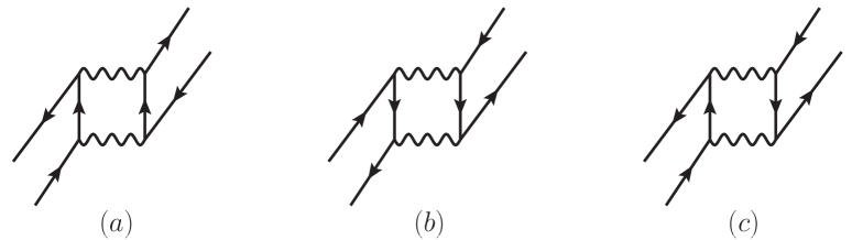
Figure 1: Diagrams contributing to the second-order quasiparticle interaction (exchange terms omitted): (a) particle-particle diagram, (b) hole-hole diagram, and (c) particle-hole diagram.

In the following, we discuss the general evaluation of eqs. (14) and (15) for interactions given in the partial-wave basis. We first define the spin-averaged quasiparticle interaction $\bar{\cal F}(pST)$, which is obtained from the full quasiparticle interaction by averaging over the spin-substates:

$$\bar{\cal F}(pST)=\frac{1}{2S+1}\sum_{m_{s}}{\cal F}(pSm_{s}TT_{z}),$$ (17)

where $p=\frac{1}{2}|\vec{p}_{1}-\vec{p}_{2}\,|=k_{F}\sin\theta/2$, and in ${\cal F}(pSm_{s}TT_{z})$ the spins and isospins of the two quasiparticles are coupled to total spin $S=0,1$ and total isospin $T=0,1$. We take an isospin-symmetric two-body potential and thus the quasiparticle interaction is independent of $T_{z}$. The first-order contribution to the central part of the quasiparticle interaction is then obtained by summing over the allowed partial wave matrix elements:

$$\bar{\cal F}^{(1)}(pST)=\frac{1}{2S+1}\sum_{J,l}(2J+1)\left\langle plSJT\right|\bar{V}\left|plSJT\right\rangle\,.$$ (18)

Note that there is an additional factor of $4\pi$ in eq. (41) in ref. schwenk02 and eq. (28) in ref. holt07 due to a different normalization convention. From eq. (18) we can project out the individual components of the quasiparticle interaction using the appropriate linear combinations of $\bar{\cal F}(pST)$ with $S=0,1$ and $T=0,1$:

$$f(p) = \;\;\,\frac{1}{16}\bar{\cal F}^{(1)}(p00)+\frac{3}{16}\bar{\cal F}^{(1)}(p01)+\frac{3}{16}\bar{\cal F}^{(1)}(p10)+\frac{9}{16}\bar{\cal F}^{(1)}(p11)$$

$$g(p) = -\frac{1}{16}\bar{\cal F}^{(1)}(p00)-\frac{3}{16}\bar{\cal F}^{(1)}(p01)+\frac{1}{16}\bar{\cal F}^{(1)}(p10)+\frac{3}{16}\bar{\cal F}^{(1)}(p11)$$

$$f^{\prime}(p) = -\frac{1}{16}\bar{\cal F}^{(1)}(p00)+\frac{1}{16}\bar{\cal F}^{(1)}(p01)-\frac{3}{16}\bar{\cal F}^{(1)}(p10)+\frac{3}{16}\bar{\cal F}^{(1)}(p11)$$

$$g^{\prime}(p) = \;\;\,\frac{1}{16}\bar{\cal F}^{(1)}(p00)-\frac{1}{16}\bar{\cal F}^{(1)}(p01)-\frac{1}{16}\bar{\cal F}^{(1)}(p10)+\frac{1}{16}\bar{\cal F}^{(1)}(p11).$$ (19)

The leading-order expressions, eqs. (18) and (19), give the full $p$-dependence (i.e., angular dependence) of the quasiparticle interaction, and therefore one can project out the density-dependent Landau parameters for arbitrary $L$:

$$X_{L}=2(2L+1)\int_{0}^{k_{F}}dp\frac{p}{k_{F}^{2}}X(p)P_{L}(1-2p^{2}/k_{F}^{2}).$$ (20)

For the second-order contributions to the quasiparticle interaction, the complete $p$-dependence is in general not easily obtained (e.g., for the particle-hole term). We instead compute the Landau parameters for each $L$ separately, choosing the total momentum vector to be aligned with the $z$-axis. In the following, the two quasiparticle momenta are labeled $\vec{p}_{1}$ and $\vec{p}_{2}$, while the intermediate-state momenta are labeled $\vec{k}_{3}$ and $\vec{k}_{4}$. For the particle-particle contribution one finds

$${\cal F}^{(2)pp}_{L}(Sm_{s}T)=\frac{2L+1}{4\pi^{2}k_{F}^{2}}\sum_{\begin{subarray}{c}l_{1}l_{2}l_{3}l_{4}mm^{\prime}\\ m_{s}^{\prime}JJ^{\prime}M\end{subarray}}\int_{0}^{k_{F}}dp\,p\int_{p}^{\infty}dq\,q^{2}N(l_{1}ml_{2}m^{\prime}l_{3}ml_{4}m^{\prime})P_{l_{1}}^{m}(0)P_{l_{3}}^{m}(0)$$

$$\hskip 21.68121pt\times\frac{M_{N}}{p^{2}-q^{2}}i^{l_{2}+l_{3}-l_{1}-l_{4}}{\cal C}^{JM}_{l_{1}msm_{s}}{\cal C}^{JM}_{l_{2}m^{\prime}sm_{s}^{\prime}}{\cal C}^{J^{\prime}M}_{l_{3}msm_{s}}{\cal C}^{J^{\prime}M}_{l_{4}m^{\prime}sm_{s}^{\prime}}\int^{{\rm min}\{x_{0},1\}}_{{\rm max}\{-x_{0},-1\}}d\cos\theta_{q}\,P_{l_{2}}^{m^{\prime}}(\cos\theta_{q})P_{l_{4}}^{m^{\prime}}(\cos\theta_{q})$$

$$\hskip 21.68121pt\times\langle pl_{1}SJMT|\bar{V}|ql_{2}SJMT\rangle\langle ql_{4}SJ^{\prime}MT|\bar{V}|pl_{3}SJ^{\prime}MT\rangle P_{L}(1-2p^{2}/k_{F}^{2}),$$ (21)

where $P_{l}^{m}$ are associated Legendre functions, $\vec{p}=(\vec{p}_{1}-\vec{p}_{2})/2$, $\vec{q}=(\vec{k}_{3}-\vec{k}_{4})/2$, $x_{0}=(q^{2}-p^{2})/2q\sqrt{k_{F}^{2}-p^{2}}$ and $N(l_{1}ml_{2}m^{\prime}l_{3}ml_{4}m^{\prime})=N_{l_{1}}^{m}N_{l_{2}}^{m^{\prime}}N_{l_{3}}^{m}N_{l_{4}}^{m^{\prime}}$ with $N_{l}^{m}=\sqrt{(2l+1)(l-m)!/(l+m)!}$. Similarly, for the hole-hole diagram one obtains

$${\cal F}^{(2)hh}_{L}(Sm_{s}T)=\frac{2L+1}{4\pi^{2}k_{F}^{2}}\sum_{\begin{subarray}{c}l_{1}l_{2}l_{3}l_{4}mm^{\prime}\\ m_{s}^{\prime}JJ^{\prime}M\end{subarray}}\int_{0}^{k_{F}}dp\,p\int_{0}^{p}dq\,q^{2}N(l_{1}ml_{2}m^{\prime}l_{3}ml_{4}m^{\prime})P_{l_{1}}^{m}(0)P_{l_{3}}^{m}(0)$$

$$\hskip 21.68121pt\times\frac{M_{N}}{q^{2}-p^{2}}i^{l_{2}+l_{3}-l_{1}-l_{4}}{\cal C}^{JM}_{l_{1}msm_{s}}{\cal C}^{JM}_{l_{2}m^{\prime}sm_{s}^{\prime}}{\cal C}^{J^{\prime}M}_{l_{3}msm_{s}}{\cal C}^{J^{\prime}M}_{l_{4}m^{\prime}sm_{s}^{\prime}}\int^{{\rm min}\{-x_{0},1\}}_{{\rm max}\{x_{0},-1\}}d\cos\theta_{q}\,P_{l_{2}}^{m^{\prime}}(\cos\theta_{q})P_{l_{4}}^{m^{\prime}}(\cos\theta_{q})$$

$$\hskip 21.68121pt\times\langle pl_{1}SJMT|\bar{V}|ql_{2}SJMT\rangle\langle ql_{4}SJ^{\prime}MT|\bar{V}|pl_{3}SJ^{\prime}MT\rangle P_{L}(1-2p^{2}/k_{F}^{2}).$$ (22)

Averaging over the spin substates and employing eq. (19) with the substitution $\bar{\cal F}^{(1)}\rightarrow\bar{\cal F}^{(2)}$ again yields the individual spin and isospin components of the quasiparticle interaction. The evaluation of the particle-hole diagram proceeds similarly; however, in this case the coupling of the two quasiparticles to total spin (and isospin) requires an additional step. Coupling to states with $m_{s}=0$ is achieved by taking the combinations (neglecting isospin for simplicity)

$${\cal F}^{(2)ph}({\vec{p}}_{1}{\vec{p}}_{2};S=1/2\pm 1/2,m_{s}=0)=-2\sum_{34}\left[\langle\vec{p}_{1}\vec{k}_{3}\uparrow s_{3}|\bar{V}|\vec{p}_{2}\vec{k}_{4}\downarrow s_{4}\rangle\langle\vec{p}_{2}\vec{k}_{4}\downarrow s_{4}|\bar{V}|\vec{p}_{1}\vec{k}_{3}\uparrow s_{3}\rangle\right.$$

$$\pm\left.\langle\vec{p}_{1}\vec{k}_{3}\uparrow s_{3}|\bar{V}|\vec{p}_{2}\vec{k}_{4}\uparrow s_{4}\rangle\langle\vec{p}_{2}\vec{k}_{4}\downarrow s_{4}|\bar{V}|\vec{p}_{1}\vec{k}_{3}\downarrow s_{3}\rangle\right]\frac{n_{3}(1-n_{4})}{\epsilon_{1}+\epsilon_{3}-\epsilon_{2}-\epsilon_{4}}.$$ (23)

We provide the expression for ${\cal F}^{(2)ph}_{0}$ (corresponding to $L=0$) in uncoupled quasiparticle spin and isospin states, appopriate for evaluating the first term in eq. (23), which can be easily generalized in order to obtain the second term. We find

$${\cal F}^{(2)ph}_{0}(s_{1}s_{2}t_{1}t_{2})=-\frac{1}{\pi^{2}k_{F}^{2}}\sum_{\begin{subarray}{c}s_{3}s_{4}t_{3}t_{4}\\ l_{1}l_{2}l_{3}l_{4}mm^{\prime}\\ SJMTS^{\prime}J^{\prime}T^{\prime}\end{subarray}}\int_{0}^{2k_{F}}dp^{\prime}\int_{k_{F}-p^{\prime}/2}^{\sqrt{k_{F}^{2}-{p^{\prime}}^{2}/4}}dp\,p\int_{\sqrt{k_{F}^{2}-{p^{\prime}}^{2}/4}}^{k_{F}+p^{\prime}/2}dq\,q\,N(l_{1}ml_{2}m^{\prime}l_{3}ml_{4}m^{\prime})$$

$$\times\frac{M_{N}}{p^{2}-q^{2}}P_{l_{1}}^{m}(\cos\theta_{p})P_{l_{3}}^{m}(\cos\theta_{p})P_{l_{2}}^{m^{\prime}}(\cos\theta_{q})P_{l_{4}}^{m^{\prime}}(\cos\theta_{q})i^{l_{2}+l_{3}-l_{1}-l_{4}}{\cal C}^{JM}_{l_{1}mSm_{s}}{\cal C}^{JM}_{l_{2}m^{\prime}Sm_{s}^{\prime}}{\cal C}^{J^{\prime}M}_{l_{3}mS^{\prime}m_{s}}{\cal C}^{J^{\prime}M}_{l_{4}m^{\prime}S^{\prime}m_{s}^{\prime}}$$

$$\times{\cal C}(s_{1}s_{2}s_{3}s_{4}){\cal C}(t_{1}t_{2}t_{3}t_{4})\langle pl_{1}SJMT|\bar{V}|ql_{2}SJMT\rangle\langle ql_{4}S^{\prime}J^{\prime}MT^{\prime}|\bar{V}|pl_{3}S^{\prime}J^{\prime}MT^{\prime}\rangle,$$ (24)

where now $\vec{p}=(\vec{p}_{1}-\vec{k}_{3})/2$, $\vec{q}=(\vec{p}_{2}-\vec{k}_{4})/2$, and the total momentum $\vec{p}^{\,\prime}=\vec{p}_{1}+\vec{k}_{3}=\vec{p}_{2}+\vec{k}_{4}$. The angle $\theta_{p}$ between $\vec{p}$ and $\vec{p}^{\,\prime}$ is fixed (via $|\vec{p}_{1}\,|=k_{F}$ together with $\vec{p}_{1}=\vec{p}^{\,\prime}/2+\vec{p}$ ) by the relation $pp^{\prime}\cos\theta_{p}=k_{F}^{2}-p^{2}-{p^{\prime}}^{2}/4$, and analogously for the angle $\theta_{q}$ between $\vec{q}$ and $\vec{p}^{\,\prime}$. The combination of spin Clebsch-Gordan coefficients that arises in the above expression is denoted by

$${\cal C}(s_{1}s_{2}s_{3}s_{4})={\cal C}^{Sm_{s}}_{\frac{1}{2}s_{1}\frac{1}{2}s_{3}}{\cal C}^{Sm_{s}^{\prime}}_{\frac{1}{2}s_{2}\frac{1}{2}s_{4}}{\cal C}^{S^{\prime}m_{s}}_{\frac{1}{2}s_{1}\frac{1}{2}s_{3}}{\cal C}^{S^{\prime}m_{s}^{\prime}}_{\frac{1}{2}s_{2}\frac{1}{2}s_{4}},$$ (25)

and likewise for the combination of isospin Clebsch-Gordan coefficients. In computing the particle-hole term for $L>0$, we use

$$P_{L}(\hat{p}_{1}\cdot\hat{p}_{2})=P_{L}\left(\frac{1}{4k_{F}^{2}}{p^{\,\prime}}^{2}+\frac{1}{2k_{F}^{2}}p^{\,\prime}(p\cos\theta_{p}+q\cos\theta_{q})+\frac{pq}{k_{F}^{2}}\cos\theta_{pq}\right),$$ (26)

and employ the addition theorem for spherical harmonics to write $\cos\theta_{pq}$ in terms of $\cos\theta_{p}$, $\cos\theta_{q}$ and an azimuthal angle $\phi$. The involved integral $\int_{0}^{2\pi}d\phi$ gives different selection rules for the $m,m^{\prime}$ values of the associated Legendre functions in eq. (24). In deriving eqs. (21)–(24), we have assumed that the intermediate-state energies in eq. (15) are those of free particles: $\epsilon_{k}=\vec{k}^{2}/2M_{N}$. Later we will include the first-order correction to the dispersion relation arising from the in-medium self-energy, which leads to the substitution $M_{N}\rightarrow M^{*}$ in the above equations.

III Calculations and results

III.1 Prelude: One boson exchange interactions as test cases

The numerical computation of the quasiparticle interaction at second order is obviously quite intricate, and truncations in the number of included partial waves and in the momentum-space integrations are necessary. In such a situation it is very helpful to have available analytical results for simple model interactions in order to test the accuracy of the numerical calculations. For that purpose we derived in this subsection analytical expressions for the quasiparticle interaction up to second order arising from (i) massive scalar-isoscalar boson exchange and (ii) pion exchange modified by squaring the static propagator. We omit all technical details of these calculations which can be found (for $L=0$) in ref. kaiser06 for the case of tree-level and one-loop (i.e., second-order) pion-exchange. In the present treatment the second-order quasiparticle interaction is organized differently than in eq. (15). The explicit decomposition of the in-medium nucleon propagator into a particle and hole propagator is replaced by the sum of a “vacuum” and “medium insertion” component:

$$G(p_{0},\vec{p}\,) = i\left(\frac{\theta(|\vec{p}\,|-k_{F})}{p_{0}-\vec{p}^{\,\,2}/2M_{N}+i\epsilon}+\frac{\theta(k_{F}-|\vec{p}\,|)}{p_{0}-\vec{p}^{\,\,2}/2M_{N}-i\epsilon}\right)$$ (27)

$$= \frac{i}{p_{0}-\vec{p}^{\,\,2}/2M_{N}+i\epsilon}-2\pi\delta(p_{0}-\vec{p}^{\,\,2}/2M_{N})\theta(k_{F}-|\vec{p}\,|),$$

and the organization is now in the number of medium insertions rather than in terms of particle and hole intermediate states. The central parts of the quasiparticle interaction are constructed for any $L$ through an angle-averaging procedure

$${\cal F}_{L}(k_{F}) = \frac{2L+1}{(4\pi)^{2}}\int d\Omega_{1}d\Omega_{2}\langle\vec{p}_{1}\vec{p}_{2}|V_{\rm eff}|\vec{p}_{1}\vec{p}_{2}\rangle P_{L}(\hat{p}_{1}\cdot\hat{p}_{2})$$ (28)

$$= f_{L}(k_{F})+g_{L}(k_{F})\vec{\sigma}_{1}\cdot\vec{\sigma}_{2}+f^{\prime}_{L}(k_{F})\vec{\tau}_{1}\cdot\vec{\tau}_{2}+g^{\prime}_{L}(k_{F})\vec{\sigma}_{1}\cdot\vec{\sigma}_{2}\,\vec{\tau}_{1}\cdot\vec{\tau}_{2}\,.$$

In this equation $V_{\rm eff}$ represents the effective model interaction computed up to one-loop order (second order).

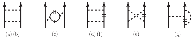
Figure 2: Diagrammatic contributions to the second-order quasiparticle interaction in nuclear matter organized in the number of medium insertions (symbolized by the short double lines). Crossed diagrams and additional reflected diagrams are not shown. The labels (b) and (f) refer to the crossed terms of (a) and (d).

We first consider as a generic example the exchange of a scalar-isoscalar boson with mass $m_{s}$ and coupling constant $g_{s}$ (to the nucleon). In momentum and coordinate space it gives rise to central potentials of the form

$$V_{C}(q)=-\frac{g_{s}^{2}}{m_{s}^{2}+q^{2}}\,,\qquad\widetilde{V}_{C}(r)=-\frac{g_{s}^{2}}{4\pi}\frac{e^{-m_{s}r}}{r}\,.$$ (29)

For the first-order contributions to the $L=0,1$ Landau parameters one finds

$${\cal F}^{(1)}_{0}(k_{F})={g_{s}^{2}\over m_{s}^{2}}\bigg{[}-1+(1+\bm{\sigma})(1+\bm{\tau})\,{\ln(1+4u^{2})\over 16u^{2}}\bigg{]}\,,$$ (30)

$${\cal F}^{(1)}_{1}(k_{F})=(1+\bm{\sigma})(1+\bm{\tau}){3g_{s}^{2}\over 32m_{s}^{2}u^{4}}\Big{[}(1+2u^{2})\ln(1+4u^{2})-4u^{2}\Big{]}\,,$$ (31)

where $\bm{\sigma}=\vec{\sigma}_{1}\cdot\vec{\sigma}_{2}$ and $\bm{\tau}=\vec{\tau}_{1}\cdot\vec{\tau}_{2}$ are short-hand notations for the spin-spin and isospin-isospin operators. The dimensionless variable $u=k_{F}/m_{s}$ denotes the ratio of the Fermi momentum $k_{F}$ to the scalar boson mass $m_{s}$. Note that in this approach both direct and crossed diagrams can contribute. The crossed diagrams have to be multiplied by the negative product of the spin- and isospin-exchange operators $-(1+\bm{\sigma})(1+\bm{\tau})/4$. At second order there are five classes of diagrammatic contributions, shown in Fig. 2, to the quasiparticle interaction. The direct terms from iterated (second order) boson exchange, see Fig. 2(a), read

$${\cal F}^{(2a)}_{0}(k_{F})=-{g_{s}^{4}M_{N}\over 32\pi m_{s}^{3}}\,{\ln(1+4u^{2})\over u^{2}}\,,$$ (32)

$${\cal F}^{(2a)}_{1}(k_{F})={3g_{s}^{4}M_{N}\over 64\pi m_{s}^{3}u^{4}}\Big{[}4u^{2}-(1+2u^{2})\ln(1+4u^{2})\Big{]}\,,$$ (33)

whereas the corresponding crossed terms (b) have the form

$${\cal F}^{(2b)}_{0}(k_{F})=(1+\bm{\sigma})(1+\bm{\tau}){g_{s}^{4}M_{N}\over 16\pi m_{s}^{3}}\int_{0}^{u}\!\!dx\,{\arctan 2x-\arctan x\over u^{2}(1+2x^{2})}\,,$$ (34)

$${\cal F}^{(2b)}_{1}(k_{F})=(1+\bm{\sigma})(1+\bm{\tau}){3g_{s}^{4}M_{N}\over 16\pi m_{s}^{3}}\int_{0}^{u}\!\!dx\,{u^{2}-2x^{2}\over u^{4}(1+2x^{2})}\big{[}\arctan 2x-\arctan x\big{]}\,.$$ (35)

The coupling of the exchanged boson to nucleon-hole states, Fig. 2(c), gives rise to nonvanishing crossed terms which read

$${\cal F}^{(2c)}_{0}(k_{F})=(1+\bm{\sigma})(1+\bm{\tau}){g_{s}^{4}M_{N}\over 4\pi^{2}m_{s}^{3}u^{2}}\int_{0}^{u}\!\!dx\,{1\over(1+4x^{2})^{2}}\bigg{[}2ux+(u^{2}-x^{2})\ln{u+x\over u-x}\bigg{]}\,,$$ (36)

$${\cal F}^{(2c)}_{1}(k_{F})=(1+\bm{\sigma})(1+\bm{\tau}){3g_{s}^{4}M_{N}\over 4\pi^{2}m_{s}^{3}u^{4}}\int_{0}^{u}\!\!dx\,{u^{2}-2x^{2}\over(1+4x^{2})^{2}}\bigg{[}2ux+(u^{2}-x^{2})\ln{u+x\over u-x}\bigg{]}\,.$$ (37)

Pauli blocking occurs in the planar- and crossed-box diagrams, Fig. 2(d)–(e), and for the sum of their direct terms one finds the forms

$${\cal F}^{(2d+2e)}_{0}(k_{F})={2g_{s}^{4}M_{N}\over\pi^{2}m_{s}^{3}u^{2}}\int_{0}^{u}\!\!dx\,{x\over(1+4x^{2})^{2}}\bigg{[}u\ln{u\over u-x}+x\ln{u-x\over x}\bigg{]}\,,$$ (38)

$${\cal F}^{(2d+2e)}_{1}(k_{F}) = {g_{s}^{4}M_{N}\over\pi^{2}m_{s}^{3}u^{4}}\int_{0}^{u}\!\!dx\,{x\over(1+4x^{2})^{2}}\bigg{[}2ux(x-u)+2u^{3}\ln{u\over u-x}$$ (39)

$$\qquad\qquad\quad+3x(u^{2}-x^{2})\ln{u^{2}-x^{2}\over x^{2}}+2x^{3}\ln{u-x\over x}\bigg{]}\,.$$

On the other hand, the crossed terms of the planar-box diagram with Pauli blocking, see Fig. 2(f) yield

$${\cal F}^{(2f)}_{0}(k_{F}) = -(1+\bm{\sigma})(1+\bm{\tau}){g_{s}^{4}M_{N}\over 4\pi^{2}m_{s}^{3}u^{2}}\int_{0}^{u}\!\!dx\,{x\over 1+4x^{2}}$$ (40)

$$\times\int_{0}^{u-x}\!\!\!dy\,{1\over\sqrt{R}}\ln{u\sqrt{R}+(1-4xy)(x-y)\over u\sqrt{R}+(4xy-1)(x-y)}\,,$$

$${\cal F}^{(2f)}_{1}(k_{F}) = -(1+\bm{\sigma})(1+\bm{\tau}){3g_{s}^{4}M_{N}\over 64\pi^{2}m_{s}^{3}u^{4}}\int_{0}^{u}\!\!dx\Bigg{\{}\ln^{2}{1+(u+x)^{2}\over 1+(u-x)^{2}}+{8x\over 1+4x^{2}}\bigg{[}u\ln{4(u-x)\over u+x}$$ (41)

$$-x\ln{u^{2}-x^{2}\over x^{2}}+\int_{0}^{u-x}\!\!\!dy\,{1+2u^{2}-4x^{2}\over\sqrt{R}}\ln{u\sqrt{R}+(1-4xy)(x-y)\over u\sqrt{R}+(4xy-1)(x-y)}\bigg{]}\Bigg{\}}\,,$$

with the auxiliary polynomial $R=4u^{2}+(4x^{2}-1)(4y^{2}-1)$. Finally, the density-dependent vertex correction to one-boson exchange, Fig. 2(g), provides a nonzero contribution only in the crossed diagram. The corresponding expressions for the $L=0,1$ Landau parameters read

$${\cal F}^{(2g)}_{0}(k_{F})=-(1+\bm{\sigma})(1+\bm{\tau}){g_{s}^{4}M_{N}\over 16\pi^{2}m_{s}^{3}u^{2}}\int_{0}^{u}\!\!dx\,{\ln(1+4x^{2})\over\sqrt{1+4u^{2}-4x^{2}}}\ln{(u\sqrt{1+4u^{2}-4x^{2}}+x)^{2}\over(1+4u^{2})(u^{2}-x^{2})}\,,$$ (42)

$${\cal F}^{(2g)}_{1}(k_{F}) = (1+\bm{\sigma})(1+\bm{\tau}){3g_{s}^{4}M_{N}\over 32\pi^{2}m_{s}^{3}u^{4}}\int_{0}^{u}\!\!dx\ln(1+4x^{2})\bigg{\{}\ln{u+x\over u-x}$$ (43)

$$-{1+2u^{2}\over\sqrt{1+4u^{2}-4x^{2}}}\ln{(u\sqrt{1+4u^{2}-4x^{2}}+x)^{2}\over(1+4u^{2})(u^{2}-x^{2})}\bigg{\}}\,.$$

Since at most double integrals over well-behaved functions are involved in the expressions in eqs. (30)–(43), they can be evaluated easily to high numerical precision. After summing them together, they provide a crucial check for our calculation of the second-order quasiparticle interaction in the partial wave basis (see Section II.2). We set the scalar boson mass $m_{s}=500$ MeV and coupling constant $g_{s}=2.5$ and work with the partial wave matrix elements following from the central potential $V_{C}(q)$ in eq. (29).

Table 1 shows the dimensionful Fermi liquid parameters (labeled ‘Exact’) as obtained from the above analytical formulas at nuclear matter saturation density ($k_{F}=1.33$ fm^-1). Due to the simple spin and isospin dependence of the underlying interaction the constraint $g_{L}=f_{L}^{\prime}=g_{L}^{\prime}$ holds. For comparison we show also the first- and second-order results obtained with the general partial wave expansion. The second-order terms are further subdivided into particle-particle, hole-hole and particle-hole contributions. We find agreement between both methods to within 1% or better for all $L=0,1$ Fermi liquid parameters. In order to achieve this accuracy, the expansions must be carried out through at least the lowest 15 partial waves.

Scalar-isoscalar boson exchange ($k_{F}=1.33$ fm-1)
	$f_{0}$ [fm2]	$g_{0}$ [fm2]	$f^{\prime}_{0}$ [fm2]	$g^{\prime}_{0}$ [fm2]	$f_{1}$ [fm2]	$g_{1}$ [fm2]	$f^{\prime}_{1}$ [fm2]	$g^{\prime}_{1}$ [fm2]
1st	$-0.809$	0.164	0.164	0.164	0.060	0.060	0.060	0.060
2nd(pp)	$-0.186$	0.056	0.056	0.056	0.038	$-0.006$	$-0.006$	$-0.006$
2nd(hh)	$-0.033$	0.010	0.010	0.010	0.042	$-0.013$	$-0.013$	$-0.013$
2nd(ph)	0.198	0.061	0.061	0.061	0.100	0.085	0.085	0.085
Total	$-0.830$	0.291	0.291	0.291	0.240	0.127	0.127	0.127
Exact	$-0.830$	0.292	0.292	0.292	0.242	0.127	0.127	0.127

Table 1: Fermi liquid parameters ($L=0,1$) for a scalar-isoscalar boson-exchange interaction with parameters described in the text. The exact results at $k_{F}=1.33$ fm^-1 obtained from our derived analytical expressions are compared to the numerical results computed via a partial wave expansion.

A feature of all realistic NN interactions is the presence of a strong tensor force, which results in mixing matrix elements between spin-triplet states differing by two units of orbital angular momentum. At second order these mixing matrix elements generate substantial contributions to the $L=0,1$ Fermi liquid parameters. In order to test the numerical accuracy of our partial wave expansion scheme for the additional complexity arising from tensor forces, we consider now the quasiparticle interaction in nuclear matter generated by (modified) “pion” exchange. To be specific we take a nucleon-nucleon potential in momentum space of the form

$$V_{T}(\vec{q}\,)=-\frac{g^{2}}{(m_{\pi}^{2}+q^{2})^{2}}\,\vec{\sigma}_{1}\cdot\vec{q}\,\,\vec{\sigma}_{2}\cdot\vec{q}\,\,\vec{\tau}_{1}\cdot\vec{\tau}_{2}\,,$$ (44)

where $g$ is a dimensionless coupling constant and $m_{\pi}$ a variable “pion” mass. The isovector spin-spin and tensor potentials in coordinate space following from $V_{T}(\vec{q}\,)$ read

$$\widetilde{V}_{S}(r)=\frac{g^{2}}{24\pi}\frac{e^{-m_{\pi}r}}{r}(m_{\pi}r-2)\,,\qquad\widetilde{V}_{T}(r)=\frac{g^{2}}{24\pi}\frac{e^{-m_{\pi}r}}{r}(1+m_{\pi}r)\,.$$ (45)

The basic motivation for squaring the propagator in eq. (44) is to tame the tensor potential at short distances, and thereby one avoids the linear divergence that would otherwise occur in iterated (second-order) one-pion-exchange. In the presence of non-convergent loop integrals, analytical and numerical treatments become difficult to match properly. Let us now enumerate the contributions at first and second order to the $L=0,1$ Landau parameters as they arise from modified “pion” exchange.

The first-order contributions read

$${\cal F}^{(1)}_{0}(k_{F})=(3-\bm{\sigma})(3-\bm{\tau}){g^{2}\over 12m_{\pi}^{2}}\bigg{[}{1\over 4u^{2}}\ln(1+4u^{2})-{1\over 1+4u^{2}}\bigg{]}\,,$$ (46)

$${\cal F}^{(1)}_{1}(k_{F})=(3-\bm{\sigma})(3-\bm{\tau}){g^{2}\over 4m_{\pi}^{2}}\bigg{[}{1+u^{2}\over 4u^{4}}\ln(1+4u^{2})-{1\over u^{2}}+{1\over 1+4u^{2}}\bigg{]}\,,$$ (47)

with the abbreviation $u=k_{F}/m_{\pi}$. For the second-order contributions we follow the labeling $(a)-(g)$ introduced previously for scalar-isoscalar boson exchange:

$${\cal F}^{(2a)}_{0}(k_{F})=(3-2\bm{\tau}){g^{4}M_{N}\over 16\pi m_{\pi}^{3}}\bigg{[}{3+16u^{2}\over 3(1+4u^{2})^{2}}-{5\over 16u^{2}}\ln(1+4u^{2})\bigg{]}\,,$$ (48)

$${\cal F}^{(2a)}_{1}(k_{F})=(3-2\bm{\tau}){g^{4}M_{N}\over 16\pi m_{\pi}^{3}}\bigg{[}{35\over 8u^{2}}-{5+24u^{2}\over(1+4u^{2})^{2}}-{5\over 32u^{4}}(7+6u^{2})\ln(1+4u^{2})\bigg{]}\,,$$ (49)

$${\cal F}^{(2b)}_{0}(k_{F}) = (5\bm{\tau}-3){g^{4}M_{N}\over 32\pi m_{\pi}^{3}}\bigg{\{}{1+\bm{\sigma}\over 8(1+u^{2})}+{1\over 3}(\bm{\sigma}-3)\bigg{[}{1\over 2u^{2}}\ln{1+2u^{2}\over 1+u^{2}}$$ (50)

$$-{1\over 1+2u^{2}}+\int_{0}^{u}\!\!dx\,{1+4x^{2}+8x^{4}\over u^{2}(1+2x^{2})^{3}}(\arctan 2x-\arctan x)\bigg{]}\bigg{\}}\,,$$

$${\cal F}^{(2b)}_{1}(k_{F}) = (5\bm{\tau}-3){g^{4}M_{N}\over 32\pi m_{\pi}^{3}}\bigg{\{}{3\over 4}(1+\bm{\sigma})\bigg{[}{1\over u^{2}}-{1\over 2(1+u^{2})}-{1\over u^{4}}\ln(1+u^{2})\bigg{]}$$ (51)

$$+(\bm{\sigma}-3)\bigg{[}{1\over 1+2u^{2}}-{1\over u^{2}}+{2+u^{2}\over 2u^{4}}\ln{1+2u^{2}\over 1+u^{2}}$$

$$+\int_{0}^{u}\!\!dx\,{u^{2}-2x^{2}\over u^{4}(1+2x^{2})^{3}}(1+4x^{2}+8x^{4})(\arctan 2x-\arctan x)\bigg{]}\bigg{\}}\,.$$

$${\cal F}^{(2c)}_{0}(k_{F})=(3-\bm{\sigma})(3-\bm{\tau}){4g^{4}M_{N}\over 3\pi^{2}m_{\pi}^{3}u^{2}}\int_{0}^{u}\!\!dx\,{x^{4}\over(1+4x^{2})^{4}}\bigg{[}2ux+(u^{2}-x^{2})\ln{u+x\over u-x}\bigg{]}\,,$$ (52)

$${\cal F}^{(2c)}_{1}(k_{F})=(3-\bm{\sigma})(3-\bm{\tau}){4g^{4}M_{N}\over\pi^{2}m_{\pi}^{3}u^{4}}\int_{0}^{u}\!\!dx\,{x^{4}(u^{2}-2x^{2})\over(1+4x^{2})^{4}}\bigg{[}2ux+(u^{2}-x^{2})\ln{u+x\over u-x}\bigg{]}\,.$$ (53)

$${\cal F}^{(2d)}_{0}(k_{F})=(3-2\bm{\tau}){16g^{4}M_{N}\over\pi^{2}m_{\pi}^{3}u^{2}}\int_{0}^{u}\!\!dx\,{x^{5}\over(1+4x^{2})^{4}}\bigg{[}u\ln{u+x\over 4(u-x)}+x\ln{u^{2}-x^{2}\over x^{2}}\bigg{]}\,,$$ (54)

$${\cal F}^{(2d)}_{1}(k_{F}) = (3-2\bm{\tau}){16g^{4}M_{N}\over\pi^{2}m_{\pi}^{3}u^{4}}\int_{0}^{u}\!\!dx\,{x^{5}\over(1+4x^{2})^{4}}\bigg{[}2u^{2}(u-x)+u^{3}\ln{u+x\over 4(u-x)}$$ (55)

$$\qquad\qquad\qquad\qquad\qquad\qquad\qquad\quad+x(3u^{2}-2x^{2})\ln{u^{2}-x^{2}\over x^{2}}\bigg{]}\,,$$

$${\cal F}^{(2e)}_{0}(k_{F})=(3+2\bm{\tau}){16g^{4}M_{N}\over\pi^{2}m_{\pi}^{3}u^{2}}\int_{0}^{u}\!\!dx\,{x^{5}\over(1+4x^{2})^{4}}\bigg{[}u\ln{4u^{2}\over u^{2}-x^{2}}-x\ln{u+x\over u-x}\bigg{]}\,,$$ (56)

$${\cal F}^{(2e)}_{1}(k_{F})=(3+2\bm{\tau}){16g^{4}M_{N}\over\pi^{2}m_{\pi}^{3}u^{4}}\int_{0}^{u}\!\!dx\,{x^{5}\over(1+4x^{2})^{4}}\bigg{[}2u(x^{2}-u^{2})+u^{3}\ln{4u^{2}\over u^{2}-x^{2}}-x^{3}\ln{u+x\over u-x}\bigg{]}\,.$$ (57)

We split the crossed terms from the planar-box diagram with Pauli blocking, see Fig. 2(f), into factorizable parts:

$${\cal F}^{(2f)}_{0}(k_{F})=(3+\bm{\sigma})(3-5\bm{\tau}){g^{4}M_{N}\over 96\pi^{2}m_{\pi}^{3}u^{2}}\int_{0}^{u}\!\!dx\bigg{[}{x-u\over 1+(u-x)^{2}}-{x+u\over 1+(u+x)^{2}}+{1\over 2x}\ln{1+(u+x)^{2}\over 1+(u-x)^{2}}\bigg{]}^{2}\,,$$ (58)

$${\cal F}^{(2f)}_{1}(k_{F})=(3+\bm{\sigma})(3-5\bm{\tau}){g^{4}M_{N}\over 96\pi^{2}m_{\pi}^{3}u^{2}}\int_{0}^{u}\!\!dx\Big{[}G_{a}^{2}+2G_{b}^{2}\Big{]}\,,$$ (59)

$$G_{a}={u+x\over 1+(u+x)^{2}}+{x-u\over 1+(u-x)^{2}}-{1\over 2u}\ln{1+(u+x)^{2}\over 1+(u-x)^{2}}\,,$$ (60)

$$G_{b}={3\over x}-G_{a}-{3\over 4ux^{2}}(1+u^{2}+x^{2})\ln{1+(u+x)^{2}\over 1+(u-x)^{2}}\,,$$ (61)

and non-factorizable parts:

$${\cal F}^{(2f^{\prime})}_{0}(k_{F}) = (\bm{\sigma}-3)(3-5\bm{\tau}){2g^{4}M_{N}\over 3\pi^{2}m_{\pi}^{3}u^{2}}\int_{0}^{u}\!\!dx\,{x^{3}\over(1+4x^{2})^{2}}\int_{0}^{u-x}\!\!\!dy\,\bigg{\{}{2u(x-y)(1+4xy)\over R\,[4(x-y)^{2}+R]}$$ (62)

$$+{1\over R^{3/2}}(u^{2}-x^{2}-y^{2}+8x^{2}y^{2})\ln{u\sqrt{R}+(1-4xy)(x-y)\over u\sqrt{R}+(4xy-1)(x-y)}\bigg{\}}\,,$$

$${\cal F}^{(2f^{\prime})}_{1}(k_{F}) = (\bm{\sigma}-3)(3-5\bm{\tau}){g^{4}M_{N}\over 64\pi^{2}m_{\pi}^{3}u^{4}}\int_{0}^{u}\!\!dx\,\Bigg{\{}\bigg{[}\ln{1+(u+x)^{2}\over 1+(u-x)^{2}}+{1\over 1+(u+x)^{2}}$$ (63)

$$-{1\over 1+(u-x)^{2}}\bigg{]}^{2}+{32x^{3}\over(1+4x^{2})^{2}}\bigg{[}u\ln{4(u-x)\over u+x}-x\ln{u^{2}-x^{2}\over x^{2}}$$

$$+\int_{0}^{u-x}\!\!\!dy\,\bigg{(}{4u(x-y)(1+4xy)(1+2u^{2}-4x^{2})\over R\,[4(x-y)^{2}+R]}+\Big{(}2(1+2u^{2}-4x^{2})$$

$$\times(u^{2}-x^{2}-y^{2}+8x^{2}y^{2})+R\Big{)}{1\over R^{3/2}}\ln{u\sqrt{R}+(1-4xy)(x-y)\over u\sqrt{R}+(4xy-1)(x-y)}\bigg{)}\bigg{]}\Bigg{\}}\,,$$

with auxiliary polynomial $R=4u^{2}+(4x^{2}-1)(4y^{2}-1)$. These two pieces, $(2f)$ and $(2f^{\prime})$, are distinguished by whether the remaining nucleon propagator can be cancelled or not by terms from the product of (momentum-dependent) $\pi N$ interaction vertices in the numerator. Finally, the density-dependent vertex corrections to modified “pion” exchange have nonzero crossed terms, which we split again into factorizable parts:

$${\cal F}^{(2g)}_{0}(k_{F})=(3-\bm{\sigma})(3-\bm{\tau}){g^{4}M_{N}\over 96\pi^{2}m_{\pi}^{3}u^{3}}\bigg{[}{4u^{2}\over 1+4u^{2}}-\ln(1+4u^{2})\bigg{]}\bigg{[}1-{1+2u^{2}\over 4u^{2}}\ln(1+4u^{2})\bigg{]}\,,$$ (64)

$${\cal F}^{(2g)}_{1}(k_{F}) = (3-\bm{\sigma})(3-\bm{\tau}){g^{4}M_{N}\over 32\pi^{2}m_{\pi}^{3}u^{5}}\bigg{[}1-{1+2u^{2}\over 4u^{2}}\ln(1+4u^{2})\bigg{]}$$ (65)

$$\times\bigg{[}3u^{2}+{u^{2}\over 1+4u^{2}}-(1+u^{2})\ln(1+4u^{2})\bigg{]}\,,$$

and non-factorizable parts:

$${\cal F}^{(2g^{\prime})}_{0}(k_{F}) = (3-\bm{\sigma})(3-\bm{\tau}){g^{4}M_{N}\over 24\pi^{2}m_{\pi}^{3}u^{2}}\int_{0}^{u}\!\!dx\,\bigg{[}{4x^{2}\over 1+4x^{2}}-\ln(1+4x^{2})\bigg{]}$$ (66)

$$\times\bigg{\{}{2ux(1+4u^{2})^{-1}\over 1+4u^{2}-4x^{2}}+{u^{2}-x^{2}\over(1+4u^{2}-4x^{2})^{3/2}}\ln{(u\sqrt{1+4u^{2}-4x^{2}}+x)^{2}\over(1+4u^{2})(u^{2}-x^{2})}\bigg{\}}\,,$$

$${\cal F}^{(2g^{\prime})}_{1}(k_{F}) = (3-\bm{\sigma})(3-\bm{\tau}){g^{4}M_{N}\over 32\pi^{2}m_{\pi}^{3}u^{4}}\int_{0}^{u}\!\!dx\,\bigg{[}{4x^{2}\over 1+4x^{2}}-\ln(1+4x^{2})\bigg{]}$$ (67)

$$\times\bigg{\{}{4ux(1+2u^{2})\over(1+4u^{2})(1+4u^{2}-4x^{2})}-\ln{u+x\over u-x}$$

$$+{1+(u^{2}-x^{2})(6+4u^{2})\over(1+4u^{2}-4x^{2})^{3/2}}\ln{(u\sqrt{1+4u^{2}-4x^{2}}+x)^{2}\over(1+4u^{2})(u^{2}-x^{2})}\bigg{\}}\,.$$

Together with the coupling constant $g=2.5$ we choose a large “pion” mass $m_{\pi}=400$ MeV in order to suppress partial wave matrix elements from the model interaction $V_{T}(\vec{q}\,)$ beyond $J=6$ in the numerical computations based on the partial wave expansion scheme.

We show in Table 2 the $L=0,1$ Fermi liquid parameters (at $k_{F}=1.33$ fm^-1) for the modified “pion” exchange interaction up to second order in perturbation theory. The summed results from the analytic formulas eqs. (46)–(67) are labeled “Exact” and compared to the results obtained by first evaluating the interaction in the partial wave basis and then using eqs. (21)-(24). As in the case of scalar-isoscalar exchange, we find excellent agreement between the two (equivalent) methods.

Modified “pion” exchange ($k_{F}=1.33$ fm-1)
	$f_{0}$ [fm2]	$g_{0}$ [fm2]	$f^{\prime}_{0}$ [fm2]	$g^{\prime}_{0}$ [fm2]	$f_{1}$ [fm2]	$g_{1}$ [fm2]	$f^{\prime}_{1}$ [fm2]	$g^{\prime}_{1}$ [fm2]
1st	0.244	$-$0.081	$-$0.081	0.027	$-$0.079	0.026	0.026	$-$0.009
2nd(pp)	$-$0.357	$-$0.062	0.269	0.104	0.018	$-$0.005	0.027	0.009
2nd(hh)	$-$0.017	$-$0.002	0.009	0.003	0.029	0.003	$-$0.014	$-$0.005
2nd(ph)	0.146	$-$0.023	0.027	0.008	0.008	0.010	0.036	$-$0.003
Total	0.017	$-$0.169	0.224	0.142	$-$0.024	0.035	0.075	$-$0.009
Exact	0.017	$-$0.169	0.224	0.142	$-$0.023	0.035	0.074	$-$0.009

Table 2: Fermi liquid parameters ($L=0,1$) for (modified) pion exchange. The exact results at $k_{F}=1.33$ fm^-1 are obtained from our derived analytical expressions and compared to the numerical results computed via a partial wave expansion.

III.2 Realistic nuclear two-body potentials

After having verified the numerical accuracy of our partial wave expansion scheme, we extend in this section the discussion to realistic nuclear two-body potentials. We start with the Idaho N³LO chiral NN interaction entem and employ renormalization group methods bogner02 ; bogner03 ; bogner10 to evolve this (bare) interaction down to a resolution scale ($\Lambda\simeq 2$ fm^-1) at which the NN interaction becomes universal. The quasiparticle interaction in nuclear matter has been studied previously with such low-momentum nuclear interactions schwenk02 ; holt07 ; kukei , but a complete second-order calculation has never been performed. Given the observed better convergence properties of low-momentum interactions in nuclear many-body calculations, we wish to study here systematically the order-by-order convergence of the quasiparticle interaction derived from low-momentum NN potentials. A complete treatment of low-momentum nuclear forces requires the consistent evolution of two- and three-body forces together. We postpone the inclusion of contributions to the quasiparticle interaction from the (chiral) three-nucleon force to upcoming work holt11 .

In Table 3 we compare the $L=0,1$ Fermi liquid parameters obtained from the bare chiral N³LO potential to those of low-momentum interactions obtained by integrating out momenta above a resolution scale of $\Lambda=2.1$ fm^-1 and $\Lambda=2.3$ fm^-1. The intermediate-state energies in the second-order diagrams are those of free nucleons $\epsilon_{k}=\vec{k}^{2}/2M_{N}$, and we include partial waves up to $J=6$ which result in well-converged $L=0,1$ Fermi liquid parameters. Comparing the results at first-order, we find a large decrease in the isotropic spin- and isospin-independent Landau parameter $f_{0}$ as the decimation scale decreases. This enhances the (apparent) instability of nuclear matter against isoscalar density oscillations. The effect results largely from integrating out some short-distance repulsion in the bare N³LO interaction. A repulsive contact interaction $V_{C}=4C$ (contributing with equal strength $4C$ in singlet and triplet $S$-waves) gives rise to a first-order quasiparticle interaction of the form

$${\cal F}_{0}^{(1)}=C(3-\vec{\sigma}_{1}\cdot\vec{\sigma}_{2}-\vec{\tau}_{1}\cdot\vec{\tau}_{2}-\vec{\sigma}_{1}\cdot\vec{\sigma}_{2}\,\vec{\tau}_{1}\cdot\vec{\tau}_{2})$$ (68)

and no contributions for $L\geq 1$. Thus, integrating out the short-distance repulsion in the chiral N³LO potential yields a large decrease in $f_{0}$ and a (three-times) weaker increase in $g_{0},f_{0}^{\prime}$, and $g_{0}^{\prime}$. The increase in $f_{0}^{\prime}$ gives rise to an increase in the nuclear symmetry energy at saturation density by approximately 20% for interactions evolved down to $\Lambda\simeq 2$ fm^-1. Overall, the scale dependence of the first-order $L=1$ Landau parameters is weaker, and in particular the two isospin-independent ($f_{1}$ and $g_{1}$) components of the $L=1$ quasiparticle interaction are almost scale independent. However, the parameter $f_{1}^{\prime}$ increases as the cutoff scale is lowered, which results according to eq. (9) in an increase in the anomalous orbital $g$-factor by 10–15%.

Idaho N3LO potential for $k_{F}=1.33$ fm-1
	$f_{0}$ [fm2]	$g_{0}$ [fm2]	$f^{\prime}_{0}$ [fm2]	$g^{\prime}_{0}$ [fm2]	$f_{1}$ [fm2]	$g_{1}$ [fm2]	$f^{\prime}_{1}$ [fm2]	$g^{\prime}_{1}$ [fm2]
1st	$-$1.274	0.298	0.200	0.955	$-$1.018	0.529	0.230	0.090
2nd(pp)	$-$1.461	0.023	0.686	0.255	0.041	$-$0.059	0.334	0.254
2nd(hh)	$-$0.271	0.018	0.120	0.041	0.276	0.041	$-$0.144	$-$0.009
2nd(ph)	1.642	$-$0.057	0.429	0.162	0.889	$-$0.143	0.130	0.142
Total	$-$1.364	0.281	1.436	1.413	0.188	0.367	0.550	0.477
$V_{\rm low-k}$($\Lambda=2.3$ fm-1) for $k_{F}=1.33$ fm-1
	$f_{0}$ [fm2]	$g_{0}$ [fm2]	$f^{\prime}_{0}$ [fm2]	$g^{\prime}_{0}$ [fm2]	$f_{1}$ [fm2]	$g_{1}$ [fm2]	$f^{\prime}_{1}$ [fm2]	$g^{\prime}_{1}$ [fm2]
1st	$-$1.793	0.357	0.394	1.069	$-$0.996	0.493	0.357	0.152
2nd(pp)	$-$0.974	$-$0.098	0.594	0.185	$-$0.129	$-$0.003	0.252	0.193
2nd(hh)	$-$0.358	0.030	0.169	0.075	0.338	0.028	$-$0.180	$-$0.042
2nd(ph)	2.102	0.095	0.588	0.254	1.512	0.003	0.204	0.329
Total	$-$1.023	0.385	1.744	1.583	0.725	0.521	0.634	0.632
$V_{\rm low-k}$($\Lambda=2.1$ fm-1) for $k_{F}=1.33$ fm-1
	$f_{0}$ [fm2]	$g_{0}$ [fm2]	$f^{\prime}_{0}$ [fm2]	$g^{\prime}_{0}$ [fm2]	$f_{1}$ [fm2]	$g_{1}$ [fm2]	$f^{\prime}_{1}$ [fm2]	$g^{\prime}_{1}$ [fm2]
1st	$-$1.919	0.327	0.497	1.099	$-$1.034	0.475	0.409	0.178
2nd(pp)	$-$0.864	$-$0.079	0.507	0.164	$-$0.130	0.011	0.236	0.174
2nd(hh)	$-$0.386	0.022	0.195	0.085	0.355	0.034	$-$0.195	$-$0.049
2nd(ph)	2.033	0.164	0.493	0.292	1.620	0.098	0.234	0.412
Total	$-$1.135	0.434	1.692	1.640	0.812	0.617	0.684	0.715

Table 3: Fermi liquid parameters ($L=0,1$) for the Idaho N³LO chiral potential as well as for the low-momentum nucleon-nucleon interaction $V_{\rm low-k}$ at a cutoff scale of $\Lambda=2.1$ and $2.3$ fm^-1.

Considering the three parts comprising the second-order quasiparticle interaction, we find large contributions from both the particle-particle ($pp$) and particle-hole ($ph$) diagrams. In particular, the $ph$ term is quite large, which suggests the need for an exact treatment of this contribution which until now has been absent in the literature. As the decimation scale is lowered, the $pp$ contribution is generally reduced while the hole-hole ($hh$) and $ph$ contributions are both increased. In previous studies, the $hh$ diagram has often been neglected since it was assumed to give a relatively small contribution to the quasiparticle interaction. However, we learn from our exact calculation that its effects are non-negligible for all of the spin-independent Landau parameters.

At second order, the contributions to $f_{0}$ are sizable and approximately cancel each other for the bare N³LO chiral NN interaction, but they become more strongly repulsive as the resolution scale $\Lambda$ is decreased. This reduces the large decrease at leading-order in $f_{0}$ effected through the renormalization group decimation, so that after including the second-order corrections, the spread in the values of $f_{0}$ for all three potentials (bare N³LO and its decimations to $\Lambda=2.1$ fm^-1 and $\Lambda=2.3$ fm^-1) is much smaller than at first order. For each of the three different potentials, the second-order terms are strongly coherent in both the $f_{0}^{\prime}$ and $g_{0}^{\prime}$ channels. In the former case, this change alone would give rise to a dramatic increase the nuclear symmetry energy $\beta$. This effect will be partly reduced through the increase in the quasiparticle effective mass $M^{*}$, which we see is now close to unity for the bare N³LO chiral interaction but which is strongly scale-dependent and enhanced above the free mass $M_{N}$ as the decimation scale is lowered. The parameter $g_{0}^{\prime}$, related to the energy of Giant Gamow-Teller resonances, is increased by approximately 50% after inclusion of the second-order diagrams. In Fig. 3 we plot the Fermi liquid parameters of $V_{\rm low-k}(\Lambda=2.1\,{\rm fm}^{-1})$ as a function of density $\rho=2k_{F}^{3}/3\pi^{2}$ from $\rho_{0}/4$ to $\rho_{0}$. We see that all of the $L=0$ parameters, together with $f_{1}$, are enhanced at lower densities.

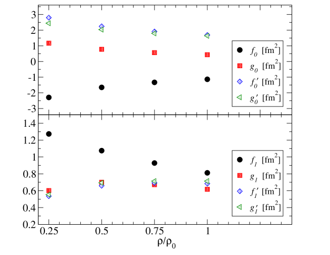
Figure 3: Density dependence of the Fermi liquid parameters for the low-momentum NN interaction $V_{\rm low-k}(\Lambda=2.1\,{\rm fm}^{-1})$. Here $\rho_{0}=0.16$ fm^-3 is the nuclear matter saturation density.

III.3 Hartree-Fock single-particle energies

We now discuss the leading-order (Hartree-Fock) contribution to the nucleon single-particle energy. The second-order contributions to the quasiparticle interaction get modified through the resulting change in the energy-momentum relation for intermediate-state nucleons. For a nucleon with momentum $\vec{k}$, the first-order (in-medium) self-energy correction reads

$$\epsilon_{k}(k_{F}) = \frac{k^{2}}{2M_{N}}+\sum_{s_{2},t_{2},|\vec{k}^{\,\prime}|\leq k_{F}}\langle\vec{k}\vec{k}^{\,\prime}s_{1}s_{2}t_{1}t_{2}|\bar{V}|\ \vec{k}\vec{k}^{\,\prime}s_{1}s_{2}t_{1}t_{2}\rangle$$ (69)

$$= \frac{k^{2}}{2M_{N}}+\frac{1}{2\pi^{2}}\sum_{lSJT}(2T+1)(2J+1)\int^{(k+k_{F})/2}_{{\rm max}\{0,(k-k_{F})/2\}}dp\,p^{2}\,{\rm min}\{2,(k_{F}^{2}-(k-2p)^{2})/4pk\}$$

$$\times \langle plSJT|\bar{V}|plSJT\rangle,$$

where $p=|\vec{k}-\vec{k}^{\,\prime}\,|/2$. In Fig. 4 we plot the single-particle energy as a function of the momentum $k$. In the left figure we show the results for all three NN interactions considered in the previous section at a Fermi momentum of $k_{F}=1.33$ fm^-1. In the right figure we consider only the low-momentum NN interaction with $\Lambda=2.1$ fm^-1 for three different densities. In all cases one can fit the dispersion relation with a parabolic form

$$\epsilon_{k}=\frac{k^{2}}{2M^{*}}+\Delta\,.$$ (70)

with $M^{*}$ the effective mass and $\Delta$ the depth of the single-particle potential. From the figure one sees that this form holds well across the relevant range of momenta $k$. In Fig. 5 we show the extracted effective mass and potential depth for the three different interactions as a function of the density. The energy shift $\Delta$ shows more sensitivity to the decimation scale $\Lambda$ than the effective mass $M^{*}$. At saturation density $\rho_{0}=0.16$ fm^-3, the variation in $\Delta$ is about 30% while the spread in $M^{*}/M_{N}$ is less than 10%. Overall, the effective mass extracted from a global fit to the momentum dependence of the single-particle energy is in good agreement with the local effective mass at the Fermi surface $k=k_{F}$, encoded in the Landau parameter $f_{1}$. The largest difference occurs for the bare Idaho N³LO potential owing to the larger momentum range over which eq. (70) is fit to the spectrum.

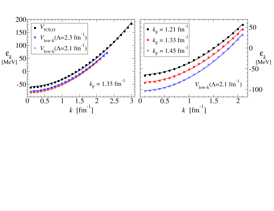
Figure 4: Single-particle energies (symbols) computed from eq. (69) and fit (lines) with the form eq. (70) characterized by an effective mass plus energy shift.

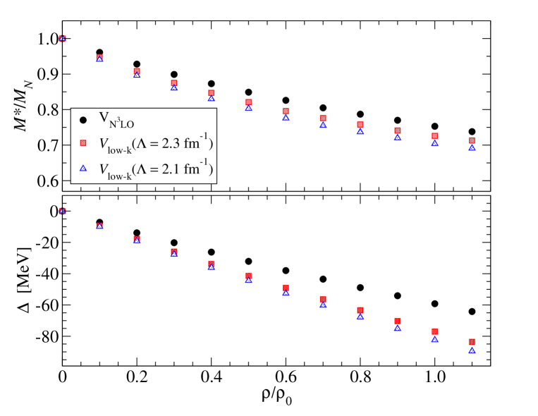
Figure 5: Parameterization of the single-particle energy $\epsilon_{k}=k^{2}/2M^{*}+\Delta$ as a function of density for three different NN potentials.

We employ the quadratic parametrization of the single-particle energy in the second-order contributions to the quasiparticle interaction eqs. (21)–(24). This greatly simplifies the inclusion of the (first-order) in-medium nucleon self energy. The second-order quasiparticle interaction is effectively multiplied by the same factor $M^{*}/M_{N}$, since the constant shift $\Delta$ cancels in the energy differences. We then compute the dimensionless Fermi liquid parameters by factoring out the density of states at the Fermi surface $N_{0}=2M^{*}k_{F}/\pi^{2}$. In Table 4 we show the results at $k_{F}=1.33$ fm^-1 for the Idaho N³LO potential as well as $V_{\rm low-k}^{\Lambda}$ for $\Lambda=2.1$ fm^-1 and $\Lambda=2.3$ fm^-1. In addition, we have tabulated the theoretical values of the different nuclear observables that can be obtained from the Fermi liquid parameters. The quasiparticle effective mass of the bare N³LO chiral NN interaction is $M^{*}/M_{N}=0.944$, but this ratio increases beyond 1 for the low-momentum NN interactions. The inclusion of self-consistent single-particle energies in the second-order diagrams reduces the very large enhancement in the effective mass seen previously in Table 3. Compared to the other three $L=0$ Landau parameters, the spin-spin interaction in nuclear matter is relatively small ($G_{0}=0.35-0.58$). Despite the strong repulsion in $F_{0}$ that arises from the second-order $ph$ diagram, we see that nuclear matter remains unstable against isoscalar density fluctuations ($F_{0}<-1$), and this behavior is enhanced in evolving the potential to lower resolution scales. The nuclear symmetry energy $\beta$ is weakly scale dependent and we find that the predicted value is within the experimental errors $\beta=(33\pm 3)$ MeV. Partly due to the rather large effective mass $M^{*}/M_{N}$ at the Fermi surface, the anomalous orbital $g$-factor comes out too small compared to the empirical value of $\delta g_{l}=0.23\pm 0.03$. The $L=0$ spin-isospin Landau parameter $G_{0}^{\prime}$ is quite large for the low-momentum NN interactions. Using the conversion factor $(g_{\pi N}/2M_{N})^{2}=1.9$ fm² one gets the values $g_{NN}^{\prime}=0.67,0.75$, and 0.77 for the bare N³LO chiral NN interaction and evolved interactions $V_{\rm low-k}^{2.3}$ and $V_{\rm low-k}^{2.1}$ respectively. These numbers are in good agreement with values of $g_{NN}^{\prime}\gtrsim 0.6$ obtained by fitting properties of giant Gamow-Teller resonances.

The above results highlight the necessity for including three-nucleon force contributions to the quasiparticle interaction both for the bare and evolved potentials. In fact it has been shown that supplementing the (low-momentum) potentials considered in this work with the leading chiral three-nucleon force produces a realistic equation of state for cold nuclear matter bogner05 ; hebeler11 . The large additional repulsion arising in the three-nucleon Hartree-Fock contribution to the energy per particle should remedy the largest deficiency observed in present calculation, namely the large negative value of the compression modulus ${\cal K}$. A detailed study of the effects of chiral three-forces (or equivalently the density-dependent NN interactions derived therefrom holt09 ; holt10 ; hebeler10 ) on the Fermi liquid parameters is presently underway.

	$F_{0}$	$G_{0}$	$F_{0}^{\prime}$	$G_{0}^{\prime}$	$F_{1}$	$G_{1}$	$F^{\prime}_{1}$	$G^{\prime}_{1}$	$M^{*}/M_{N}$	${\cal K}$ [MeV]	$\beta$ [MeV]	$\delta g_{l}$
$V_{\rm N3LO}$	$-$1.64	0.35	1.39	1.59	$-$0.13	0.50	0.58	0.47	0.96	$-$148	30.5	0.12
$V_{\rm low-k}^{2.3}$	$-$1.77	0.54	1.98	2.07	0.36	0.74	0.80	0.72	1.12	$-$152	32.5	0.07
$V_{\rm low-k}^{2.1}$	$-$1.98	0.58	1.94	2.14	0.38	0.83	0.87	0.80	1.13	$-$191	31.8	0.07

Table 4: Sum of the first- and second-order contributions to the dimensionless Fermi liquid parameters for the Idaho N³LO potential and two low-momentum NN interactions $V_{\rm low-k}^{\Lambda}$ at $k_{F}=1.33$ fm^-1. Hartree-Fock self-energy insertions, as parameterized in eq. (70), are included in the second-order diagrams.

IV Summary and conclusions

We have performed a complete calculation up to second-order for the quasiparticle interaction in nuclear matter employing both the Idaho N³LO chiral NN potential as well as evolved low-momentum NN interactions. The numerical accuracy of our results is on the order of 1% or better. This precision is tested using analytically-solvable (at second order) schematic nucleon-nucleon potentials emerging from scalar-isoscalar boson exchange and modified “pion” exchange. We have found that the first-order approximation to the full quasiparticle interaction exhibits a strong scale dependence in $f_{0}$, $f_{0}^{\prime}$, and $f_{1}^{\prime}$, which decreases the nuclear matter incompressibility ${\cal K}$ and increases the symmetry energy $\beta$ and anomalous orbital $g$-factor $\delta g_{l}$ as the resolution scale $\Lambda$ is lowered. Our second-order calculation reveals the importance of the hole-hole contribution in certain channels as well as the strong effects from the particle-hole contribution for the $f_{0}$ and $f_{1}$ Landau parameters. The total second-order contribution has a dramatic effect on the quasiparticle effective mass $M^{*}$, the nuclear matter incompressibility ${\cal K}$ and symmetry energy $\beta$, as well as the Landau-Migdal parameter $g_{0}^{\prime}$ that governs the nuclear spin-isospin response. In contrast, the components of the spin-spin quasiparticle interaction ($g_{0},g_{1}$) are dominated by the first-order contribution. We have included also the Hartree-Fock contribution to the nucleon single-particle energy, which reduces the second-order diagrams by about 30% (as a result of the replacement $M_{N}\to M^{*}$). The final set of $L=0,1$ Landau parameters representing the quasiparticle interaction in nuclear matter provides a reasonably good description of the nuclear symmetry energy $\beta$ and spin-isospin collective modes. Our calculations demonstrate, however, that the second-order quasiparticle interaction, generated from realistic two-body forces only, still leaves the nuclear many-body system instable with respect to scalar-isoscalar density fluctuations. Neither the incompressibility of nuclear matter ${\cal K}$ nor the anomalous orbital $g$-factor $\delta g_{l}$ could be reproduced satisfactorily (without the inclusion of three-nucleon forces). A detailed study of the expected improvements in the quasiparticle interaction resulting from the leading-order chiral three-nucleon force is the subject of an upcoming investigation holt11 .

References

- (1) S. Fritsch, N. Kaiser and W. Weise, Nucl. Phys. A750 (2005) 259.
- (2) S. K. Bogner, A. Schwenk, R. J. Furnstahl, and A. Nogga, Nucl. Phys. A763 (2005) 59.
- (3) L.-W. Siu, J. W. Holt, T. T. S. Kuo and G. E. Brown, Phys. Rev. C 79 (2009) 054004.
- (4) K. Hebeler, S. K. Bogner, R. J. Furnstahl, A. Nogga and A. Schwenk, Phys. Rev. C 83 (2011) 031301.
- (5) L. D. Landau, Sov. Phys. JETP, 3 (1957) 920; 5 (1957) 101; 8 (1959) 70.
- (6) A. B. Migdal and A. I. Larkin, Sov. Phys. JETP 18 (1964) 717.
- (7) A. B. Migdal, Theory of Finite Fermi Systems and Applications to Atomic Nuclei (Interscience, New York, 1967).
- (8) G. Baym and C. Pethick, Landau Fermi-Liquid Theory (Wiley & Sons, New York, 1991).
- (9) S. Babu and G.E. Brown, Ann. Phys. 78 (1973) 1.
- (10) O. Sjöberg, Ann. Phys. 78 (1973) 39.
- (11) W. H. Dickhoff, A. Faessler, H. Müther, and S. S. Wu, Nucl. Phys. A405 (1983) 534.
- (12) S. O. Bäckman, G. E. Brown, and J. A. Niskanen, Phys. Rept. 124 (1985) 1.
- (13) J. W. Holt, G. E. Brown, J. D. Holt and T. T. S. Kuo, Nucl. Phys. A785 (2007) 322.
- (14) N. Kaiser, Nucl. Phys. A768 (2006) 99.
- (15) D. R. Entem and R. Machleidt, Phys. Rev. C 66 (2002) 014002.
- (16) S. K. Bogner, T. T. S. Kuo, L. Coraggio, A. Covello, and N. Itaco, Phys. Rev. C 65 (2002) 051301(R).
- (17) S. K. Bogner, T. T. S. Kuo, and A. Schwenk, Phys. Rept. 386 (2003) 1.
- (18) S. K. Bogner, R. J. Furnstahl and A. Schwenk, Prog. Part. Nucl. Phys. 65 (2010) 94.
- (19) J. W. Holt, N. Kaiser and W. Weise, in preparation.
- (20) J. P. Blaizot, Phys. Rept. 64 (1980) 171.
- (21) D. H. Youngblood, H. L. Clark, and Y.-W. Lui, Phys. Rev. Lett. 82 (1999) 691.
- (22) M. V. Stoitsov, P. Ring and M. M. Sharma, Phys. Rev. C 50 (1994) 1445.
- (23) P. Danielewicz, Nucl. Phys. A727 (2003) 233.
- (24) A. W. Steiner, M. Prakash, J. M. Lattimer, and P. J. Ellis, Phys. Rept. 411 (2005) 325.
- (25) H. Miyazawa, Prog. Theor. Phys. 6 (1951) 801.
- (26) G. E. Brown and M. Rho, Nucl. Phys. A338 (1980) 269.
- (27) L. Trippa, G. Colò and E. Vigezzi, Phys. Rev. C 77 (2008) 061304(R).
- (28) R. Nolte, A. Baumann, K. W. Rose and M. Schumacher, Phys. Lett. B173 (1986) 388.
- (29) C. Gaarde, Nucl. Phys. A396 (1983) 127c.
- (30) T. Ericson and W. Weise, Pions and Nuclei (Clarendon Press, Oxford, 1988).
- (31) T. Suzuki and H. Sakai, Phys. Lett. B455 (1999) 25.
- (32) A. Schwenk, G. E. Brown, and B. Friman, Nucl. Phys. A703 (2002) 745.
- (33) J. Kuckei, F. Montani, H. Müther, A. Sedrakian, Nucl. Phys. A 723 (2003) 32.
- (34) J. W. Holt, N. Kaiser, and W. Weise, Phys. Rev. C 79 (2009) 054331.
- (35) J. W. Holt, N. Kaiser, and W. Weise, Phys. Rev. C 81 (2010) 024002.
- (36) K. Hebeler and A. Schwenk, Phys. Rev. C 82 (2010) 014314.