Low-Complexity Adaptive Channel Estimation over Multipath Rayleigh Fading Non-Stationary Channels Under CFO

Abstract

In this paper, we propose novel low-complexity adaptive channel estimation techniques for mobile wireless channels in presence of Rayleigh fading, carrier frequency offsets (CFO) and random channel variations. We show that the selective partial update of the estimated channel tap-weight vector offers a better trade-off between the performance and computational complexity, compared to the full update of the estimated channel tap-weight vector. We evaluate the mean-square weight error of the proposed methods and demonstrate the usefulness of its via simulation studies.

I Introduction

In wireless communications environment, signals suffer from multiple reflections while travelling from the transmitter to the receiver so that the receiver ends up getting several replicas of the transmitted signal. The reflections are received with different amplitude and phase distortions, and the overall received signal is the combined sum of all the reflections. Based on the relative phases of the reflections, the signals may add up constructively at the receiver. Furthermore, if the transmitter is moving with respect to the receiver, these destructive and constructive interferences will vary with time. Therefore, the performance of the wireless systems critically dependent on the availability of accurate channel estimation [1], [2], [3].

Eke, periodic system variations resulting from mismatches between the transmitter and receiver carrier generators can be damaging to the performance of the estimators, even for small carrier frequency offsets [4], [5]. Adaptive filtering techniques are suitable for tracking of such time variant channels. There are many adaptive filter algorithms that are widely used for channel estimation, but they either have a high mean-square error with slow convergence rate (such as, least mean square (LMS) and normalized least mean square (NLMS) algorithms) or a high computation complexity with fast convergence rate and low mean-square error (such as, recursive least square (RLS) algorithm) [6], [7], [8]. Thus, mean- square error (MSE), convergence rate and computational complexity are three important points in selecting of adaptive algorithms for channel estimation and this is considered in choice of the applied algorithms. To address these problems, Ozeki and Omeda [9] published the basic form of an affine projection algorithm (APA) and Shin and Sayed developed tracking performance analysis of a family of APA in [10]. Furthermore, in order to reduce of computational complexity, one possible way is that only part of the estimated tap-weight vector is selected for update in each time iteration. In [11], [12] and [13] adaptive filter algorithms with selective partial update method (SPU) has been shown to have low computational complexity and good performance. In this paper, based on general formalism for the family of affine projection in [10] and using the approaches that presented in [11] and [12], we present a novel algorithms with general formalism which we called it low-complexity family of affine projection algorithms based on selective partial update method. Then, we use all of these algorithms for estimation of mutipath Rayleigh fading non-stationary channels.

The rest of this paper is organized as follows. Section II describe a brief introduction on the statistics of mobile wireless channels. In Section III, we will have a breif review on some known adaptive estimators and introduce cyclic non-stationary channels model. Subsequently, the low-complexity family of affine projection algorithms based on selective partial update method will be presented in Section IV. Finally, Section V analyzes the performance evaluation of the proposed estimation approaches by computer simulation results to demonstrate the effectiveness of the proposed algorithms for fading non-stationary channels estimation in mobile wireless environments. Section VI concludes this paper.

II Mobile Wireless Multipath Channel Model

The complex baseband representation of the mobile wireless channel impulse response can be described by [14]

$$h(t,\tau)=\sum_{k=1}^{L}\gamma_{k}(t)x_{k}(\tau)\delta(\tau-\tau_{k})$$ (1)

where $\tau_{k}$ and $\gamma_{k}(t)$ are respectively the delay and path loss of the $k$-th path. $x_{k}(\tau)$ is a time-variant complex fading sequence of the $k$-th path that models the time-variations in the channel. Hence, the frequency response at time $t$ is

$$H(t,f)\triangleq\int_{-\infty}^{+\infty}h(t,\tau)e^{-j2\pi f\tau}d\tau$$ (2)

without loss of generality, the sequence $x(\tau)$ is assumed to have unit variance. Several mathematical models can be used to characterize the fading properties of $x(\tau)$ and consequently of the channel. A widely used model is known as Rayleigh fading. In this case, for each $\tau$, the amplitude $|x(\tau)|$ is assumed to have Rayleigh distribution [3]. Therefore, the sequence $\{x_{k}(\tau)\}$ are modeled as independent Rayleigh fading sequences and the channel is referred to as a multipath fading channel. In additional, the atu-correlation function of the sequence $x(\tau)$, now regarded as a random process, is modeled as a zeroth-order bessel function of the first kind, namely,

$$r(k)\triangleq Ex(\tau)x(\tau-k)=J_{0}(2\pi f_{D}T_{s}k).$$ (3)

This commonly used choice of the auto-correlation function is based on the assumption that all scatters are uniformly distributed on a circle around the receiver, so that the power spectrum of the channel fading gain $x(\tau)$, in continuous-time, would have the following well-known $U$-shaped spectrum

$$S(f)=\frac{1}{\pi f_{D}\sqrt{1-\frac{f}{f_{D}}}},~{}~{}~{}~{}~{}~{}~{}~{}~{}~{}~{}|f|\leq f_{D}$$ (4)

In equation (3), $T_{s}$ is the sampling period of the sequence $x(\tau)$, $f_{D}$ is called the maximum Doppler frequency of the Rayleigh fading channel, and the function $J_{0}$ is defined by

$$J_{0}\triangleq\frac{1}{\pi}\int_{0}^{\pi}\cos(y\sin\theta)d\theta.$$ (5)

The Doppler frequency inversely proportional to the speed of light, $c=3\times 10^{8}m/s$ and proportional to the speed of the mobile user, $\nu$, and to the carrier frequency, $f_{c}$.

Due to the motion of the vehicle, $\gamma_{k}(t)$’s are modeled to be wide-sense stationary (WSS), narrowband complex gaussian process, which are independent for different paths. Furthermore, $\gamma_{k}(t)$’s for all $k$ have the same normalized time correlation function and different average powers $\sigma_{k}^{2}$. In nonstationary channels, a first-order approximation for the variation of a Rayleigh fading coefficient $x(\tau)$ is to assume that $x(\tau)$ varies according to the auto-regressive model

$$x(\tau)=r(1)x(\tau-1)+\sqrt{1-|r(1)|^{2}}\eta(\tau)$$ (6)

where $r(1)=J_{0}(2\pi f_{D}T_{s})$ and $\eta(\tau)$ denotes a white noise process with unit-variance.

The two-ray [15], typical urban (TU), and hilly terrain (HT) [14], [16] models are three commonly used delay profiles. For the two-ray profile with equal average power on each ray, the delay spread is $t_{d}/2$ ($t_{d}=\tau_{1}-\tau_{0}$), i.e., a half of the delay different between the two rays. The delay spreads for TU and HT delay profiles are 1.06 and 5.04 $\mu$s, respectively [17].

III Overview on Some Known Adaptive Channel Estimators

Considering Fig. 1, $x(n)$ denotes a sequence that is transmitted over an unknown channel of finite impulse response $w(n)$ of order $M$. $d(n)$ and $e(n)$ are received signal and the output estimation error, respectively. Consider the received signal $d(n)$ assuming that arisen from the linear model

Figure 1: A prototypical adaptive filter setup.

$$d(n)=u(n)w_{o}(n)+v(n)$$ (7)

$$w_{o}(n)=w_{t}(n)e^{j\Psi n}$$ (8)

where $w_{t}(n)$ is an unknown channel tap-weight vector and time variant that we wish to estimate it, the term of $e^{j\Psi n}$ indicates the carrier frequency offsets [5], $v(n)$ is the measurement noise, assumed to be zero mean, white, gaussian and independent of $u(n)$, and $u(n)=[x(n),x(n-1),...,x(n-M+1)]$ denotes $1\times M$ row input regressor vectors of the channel with a positive-definite covariance matrix, $R_{u}=E[u^{*}(n)u(n)]$.

In sequel, we shall adopt a model for the variation of $w_{t}(n)$. Many models can be defined for this variation such as random-walk or Markovian models [18]. One particular model that is widely used in the adaptive filtering literature is a first order random-walk model [10], [19]. On the other hands, we know that the carrier frequency offsets between transmitters and receivers and fading phenomenon are two important trails of the mobile wireless channels. Therefore, we can use achievable model for variations of fading channels until the performance of adaptive estimators is enhanced.

For this reason, the following both cyclic and random non-stationary model for variation of channel is introduced [5], [8]

$$w_{t}(n)=w_{t}+\Xi(n)$$ (9)

where $w_{t}$ is a constant vector that represent the non-fading part of the channel, whereas $\Xi(n)$ represent the fading part of channel that it can be modeled as autoregressive (AR) process of order $\rho$ [20]. We use common AR(1) model for this process as

$$\Xi(n+1)=\alpha\Xi(n)+q(n)$$ (10)

where

$$0\leq\mid\alpha\mid<1$$

and following from [8], the sequence $q(n)$ is assumed to be i.i.d, zero-mean with autocorrelation matrix $E\{q(n)q^{*}(n)\}=Q$ and $w_{t}(n)$ have a constant mean which we shall denote by $w_{t}$, $Ew_{t}(n)\triangleq w_{t}$. In this paper, $\alpha$ and autocorrelation matrix of $q(n)$ are $J_{0}(2\pi f_{D}T_{s})$ and $Q=\sqrt{1-\alpha^{2}}I$, respectively. This non-stationary model of channel is practical in wireless communication systems and especially in channel estimation and channel equalization applications.

It is well known that the adaptive update scheme for the LMS estimate of $w_{o}(n)$ is given by [8]

$$w(n+1)=w(n)+\mu u^{*}(n)e(n)$$ (11)

where

$$e(n)=d(n)-u(n)w(n)$$

is the output estimation error at time $n$ and $\mu$ is the step size.

To increase the convergence speed of the LMS estimator, the NLMS algorithm was proposed which can be state as [8]

$$w(n+1)=w(n)+\frac{\mu}{\|u(n)\|^{2}}u^{*}(n)e(n).$$ (12)

For reducing the computational complicity, the estimated tap-weight vector $w(n)$ and the excitation vector $u(n)$ of the adaptive estimator can be partitioned into $B$ blocks with length $L$ for each blocks that $B=M/L$ and it shall be an integer which are defined as [13]

$$u(n)=[x_{1}(n),x_{2}(n),...,x_{B}(n)]$$ (13)

$$w(n)=[w_{1}^{T}(n),w_{2}^{T}(n),...,w_{B}^{T}(n)]^{T}.$$ (14)

The selective partial update NLMS algorithm for a single block update at every iteration can be derived from the solution of the following minimization problem [13]

$$\min_{w_{j}(n+1)}\|w_{j}(n+1)-w_{j}(n)\|^{2}$$ (15a)

$$subject~{}to~{}~{}d(n)=u(n)w(n+1)$$ (15b)

by using the method of Lagrange multipliers [21], the update equation for selective partial update NLMS is given by

$$w_{j}(n+1)=w_{j}(n)+\frac{\mu}{\|u_{j}\|^{2}}u_{j}^{*}(n)e(n)$$ (16)

where

$$j=\operatorname{arg\,max}\|u_{i}(n)\|^{2}$$

for $1\leqslant{i}\leqslant{B}$ and it denotes the number of blocks that should be updated at each iteration.

From [10], the general class of affine projection algorithms can be stated as

$$w(n+1) =w(n-\beta(K-1))+$$

$$\qquad{}\mu U^{*}(n)(\epsilon I+U(n)U^{*}(n))^{-1}e(n)$$ (17)

where $e(n)=d(n)-U(n)w(n-\beta(K-1))$, and

$$U(n)=[u(n),u(n-D),...,u(n-(K-1)D)]^{T}$$ (18a)

$$d(n)=[d(n),d(n-D),...,d(n-(K-1)D)]^{T}.$$ (18b)

Based on (III) and by specific choices of the parameters $\{K,D,\epsilon,\beta\}$ are resulted in different affine projection algorithms. The particular choices and their corresponding algorithms are summarized in Table I.

TABLE I: APA FAMILY ALGORITHMS

Algorithm	$K$	$\epsilon$	$\beta$	$D$
NLMS	$K=1$	$\epsilon=0$	$\beta=0$	$D=1$
APA	$K\leq{M}$	$\epsilon=0$	$\beta=0$	$D=1$
BNDR-LMS	$K=2$	$\epsilon=0$	$\beta=0$	$D=1$
R-APA	$K\leq{M}$	$\epsilon\neq 0$	$\beta=0$	$D=1$
PRA	$K\leq{M}$	$\epsilon\neq 0$	$\beta=1$	$D=1$
NLMS-OCF	$K\leq{M}$	$\epsilon=0$	$\beta=0$	$D\geq 1$

For NLMS-OCF, it is further assumed that $u(n-jD)$ is orthogonal to $u(n),u(n-D),...,u(n-(j-1)D)$ [10]. The motivation for using $D>1$ is to increase the separation, and consequently reduce the correlation. For PRA, the weight vector is updated once every $K$ iterations that $K$ is positive integer and most algorithms assume $K\leq{M}$.

IV A Low-Complexity Family of Affine Projection Algorithms

This section introduces a low-complexity family of affine projection algorithms based on selective partial update method. From [22], the generic estimated tap-weight vector update equation can be stated as

$$\boxed{w(n+1)=w(n-\beta(K-1))+\mu U^{*}(n)C(n)e(n)}$$ (19)

where $C(n)$ is the $K\times{K}$ matrix and it is obtained from Table II. This table shows that many classical and modern adaptive filter algorithms can be derived through (19).

Considering (12), the constrained optimization problem, which is solved by the proposed algorithms are given by

$$\min_{w_{h}(n+1)}\|w_{h}(n+1)-w_{h}(n)\|^{2}$$ (20a)

$$subject~{}to~{}~{}d(n)=U(n)w(n+1)$$ (20b)

where $h=\{\tau_{1},\tau_{2},...,\tau_{S}\}$ denotes the blocks that updating at every adaptation. By using the lagrange multipliers method and considering (19), the general update equation of low-complexity family of affine projection algorithms is given by

$$w_{h}(n+1)=w_{h}(n-K^{\prime})+\mu U_{h}^{*}(n)C_{h}(n)e(n)$$ (21)

where $C_{h}(n)$ is the $K\times{K}$ matrix and it is obtained from Table II, $K^{\prime}=\beta(K-1)$, and we have

$$U_{h}(n)=[U_{\tau_{1}}(n),U_{\tau_{2}}(n),...,U_{\tau_{S}}(n)]$$ (22)

$$U_{\tau_{S}}(n)=[u_{\tau_{S}}(n),u_{\tau_{S}}(n-D),...,u_{\tau_{S}}(n-(K-1)D)]^{T}$$ (23)

$$U_{i}(n)=[u_{i}(n),u_{i}(n-D),...,u_{i}(n-(K-1)D)]^{T}.$$ (24)

In above equations, $U_{h}(n)$ is the $K\times{LS}$ matrix, $U_{\tau_{S}}(n)$ is $K\times{L}$, $u_{\tau_{S}}(n)$ is $1\times{L}$ and $U_{i}(n)$ is the $K\times{L}$ matrix. For obtaining the indices of $h$, we compute the values of

$$\text{Tr}(U_{i}(n)U_{i}^{*}(n))~{}~{}~{}for~{}~{}~{}1\leq{i}\leq{B}$$ (25)

then, $S$ largest blocks are selected for updating. The $K\times{K}$ matrix $U_{i}(n)U_{i}^{*}(n)$ is assumed to be full rank (i.e., invertable). The inequality $L\geq{K}$ is a necessary condition for $U_{i}(n)U_{i}^{*}(n)$ to be full rank. Note that, for $K=1$, $\text{Tr}(U_{i}(n)U_{i}^{*}(n))$ reduces to $\|u(n)\|^{2}$. Thus, (25) is consistent with the selection criterion for the SPU-NLMS algorithm.

From (21), with different choices of the parameters $\{K,D,\epsilon,\beta\}$ and $C_{h}(n)$ from Table.II, the new adaptive estimators such as low-complexity version of BNDR-LMS, NLMS-OCF and PRA based on selective partial update method will be derived.

TABLE II: Correspondence Between Special Cases of (21) and Various Low-Complexity Adaptive Filtering Algorithms

Algorithm	$K$	$\beta$	$D$	$C(n)$	$C_{h}(n)$
LMS	$K=1$	$\beta=0$	$D=1$	$C(n)=1$	-
NLMS	$K=1$	$\beta=0$	$D=1$	$C(n)=\|u(n)\|^{-2}$	$C_{h}(n)=[U_{h}(n)U_{h}^{*}(n)]^{-1}$
APA	$K\leq{M}$	$\beta=0$	$D=1$	$C(n)=[U(n)U^{*}(n)]^{-1}$	$C_{h}(n)=[U_{h}(n)U_{h}^{*}(n)]^{-1}$
BNDR-LMS	$K=2$	$\beta=0$	$D=1$	$C(n)=[U(n)U^{*}(n)]^{-1}$	$C_{h}(n)=[U_{h}(n)U_{h}^{*}(n)]^{-1}$
R-APA	$K\leq{M}$	$\beta=0$	$D=1$	$C(n)=[\epsilon{I}+U(n)U^{*}(n)]^{-1}$	$C_{h}(n)=[\epsilon{I}+U_{h}(n)U_{h}^{*}(n)]^{-1}$
PRA	$K\leq{M}$	$\beta=1$	$D=1$	$C(n)=[\epsilon{I}+U(n)U^{*}(n)]^{-1}$	$C_{h}(n)=[\epsilon{I}+U_{h}(n)U_{h}^{*}(n)]^{-1}$
NLMS-OCF	$K\leq{M}$	$\beta=0$	$D\geq 1$	$C(n)=[U(n)U^{*}(n)]^{-1}$	$C_{h}(n)=[U_{h}(n)U_{h}^{*}(n)]^{-1}$

V Performance Evaluation by Simulation Studeis

Extensive computer simulations have been conducted to demonstrate the performance of the adaptive estimators for multipath Rayleigh fading non-stationary channel estimation. In adaptive filtering problems, recursive algorithms are used to find the channel tap-weight that produces the minimum error between the desired value and received value. Since the channel can be modeled as a tap-delay line filter, the channel estimation problem can be formulated as that of an adaptive filtering problem. Fig. 1 illustrates the process of the adaptive filtering and we can use of this process to estimate the non-stationary channel taps. The objective of the adaptive algorithm is to find the optimal tap-weight vector that gives the minimum mean-squared error [8].

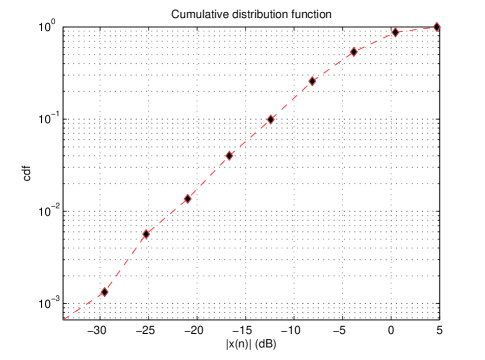
Figure 2: The cumulative distribution function of a Rayleigh fading sequence corresponding to a vehicle moving at 80Km/h.

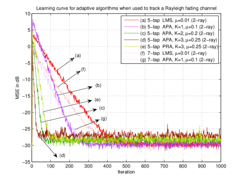
Figure 3: The first 1000 samples of a learning curve that results from tracking a Rayleigh fading non-stationary channel using LMS and family of APA algorithms.

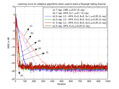
Figure 4: The first 1000 samples of a learning curve that results from tracking a Rayleigh fading non-stationary channel using LMS, APA and Low-Complexity APA algorithms.

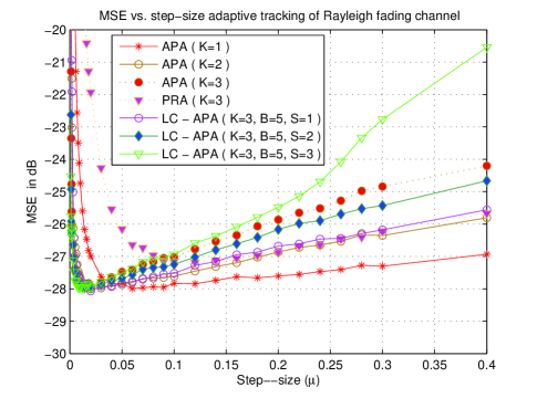
Figure 5: A plot of the tracking MSE as a function of the step-size for Rayleigh fading rays with Doppler frequency at 10Hz.

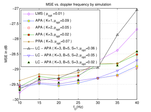
Figure 6: A plot of the tracking MSE as a function of the Doppler frequency of the Rayleigh fading rays

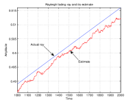
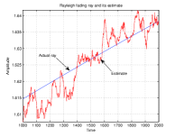
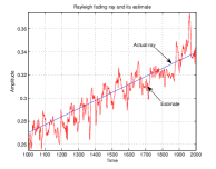
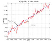
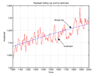
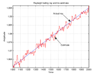
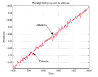
Figure 7: A plot of a typical trajectory of the amplitude of the first Rayleigh ray and its estimate. The plots zooms on the interval $1000\leq i\leq 2000$. 7 LMS algorithm with $\mu=0.01$ 7 APA algorithm with $K=1$ and $\mu=0.1$ 7 APA algorithm with $K=2$ and $\mu=0.25$ 7 PRA algorithm with $K=3$ and $\mu=0.25$ 7 LC-APA algorithm with $K=3$ , $B=5$ , $S=1$ and $\mu=0.25$ 7 LC-APA algorithm with $K=3$ , $B=5$ , $S=2$ and $\mu=0.25$ 7 LC-APA algorithm with $K=3$ , $B=5$ , $S=3$ and $\mu=0.25$.

In this paper, we consider a wireless channel with two Rayleigh fading rays; both rays are assumed to fade at the same Doppler frequency of $f_{D}=10Hz$. The channel impulse response sequence consists of two zero initial samples (i.e., an initial delay of two samples), followed by a Rayleigh fading ray, followed by another zero sample, and by a second Rayleigh fading ray and then, for another channel response, we will add two zero samples after a second Rayleigh fading ray. In other words, we are assuming a channel length of M=5 or 7 taps with only two active Rayleigh fading ray, so that the weight vector that we wish to estimate has the form

$$[~{}0~{}~{}0~{}~{}x_{2}(\tau)~{}~{}0~{}~{}x_{4}(\tau)~{}]$$ (26)

or

$$[~{}0~{}~{}0~{}~{}x_{2}(\tau)~{}~{}0~{}~{}x_{4}(\tau)~{}~{}0~{}~{}0~{}]$$ (27)

Train adaptive algorithm to estimate and track these multipath non-stationary channels. Assume random binary phase shift keying (BPSK) input signal of unit variance is transmitted across the channel and use it to excite the adaptive filter. Assume further that the output of the channel is observed in the presence of white additive Gaussian noise with variance $\sigma_{\upsilon}^{2}=10^{-3}$, sampling period $T_{s}=0.8\mu s$, $\alpha=0.9$, $\sigma^{2}_{q}=10^{-4}$ and carrier frequency offsets $\Psi=0.0001$. Fig. 2 shows the cumulative distribution function of the amplitude sequence. A plot of the learning curve of all adaptive estimators is generated by running them for 30000 iterations and averaging over 100 independent experiments and show the good performance of proposed algorithm with lower computational complexity that convergence rate of its is comparable with full update APA estimators. Figs. 3 and 4 show only the first 1000 iterations of a typical learning curves. Fig. 5 shows mean-square error (MSE) curves versus step-size for the proposed scheme and other algorithms that they are presented in this paper. In this simulation, the Doppler frequency is fixed at 10Hz for both rays, channel length $M=5$ taps, and the MSE values are obtained by averaging over 100 independent realizations.

In Fig. 6, the Doppler frequency vary from 10Hz to 40Hz in increments of 5Hz and generate a plot of the MSE as a function of the Doppler frequency. Run all adaptive estimators for 60000 iterations in each case and average the squared-error curve over 1000 independent experiments. Also, we used the optimum value of the step-size for all algorithms which we selected these optimum values from minimizing of mean-square weight error function over step-size $\mu$ . This figure shows the robustness of adaptive estimators for different values of Doppler frequency.

Fig.7 shows typical trajectory of the amplitude of the first ray and its estimate by different adaptive estimators. These plots zooms onto the interval [1000, 2000]. The results show the good tracking performance of adaptive algorithms for multipath Rayleigh fading non-stationary channels tracking and proposed method is better than LMS and APA ($K=1$) algorithms and comparable with APA ($K=3$) algorithm but our proposed method has lower computational complexity than ordinary family of APA algorithms.

VI Conclusion

The tracking performance of the new low-complexity family of affine projection algorithms in the presence of carrier frequency offsets and random channel nonstationarities was studied in this paper. A general formalism for proposed algorithms was also developed, and the mean-square weight error under steady-state conditions was analyzed. The performance of our methods were compared with those of some other estimators. The proposed schemes presented a good trade-off between the performance and the computational complexity. The simulation results were included to demonstrate our claims.

Appendix A The Mean-Square Weight Error of the Cyclic Non-Stationary Channel Estimation

To find the mean-square weight error of low-complexity family of affine projection algorithms, following from [8], [7], let us praise a definition and a assumption as follows

Definition: For the cyclic model of channel nonstationarities , the weight-error vector is $\varepsilon(n)=w_{t}(n)e^{j\Psi n}-w_{h}(n)$, and a priori and a posteriori estimation errors are defined as $e_{a}(n)=U_{h}(n)\varepsilon(n-K^{\prime})$, $e_{p}(n)=U_{h}(n)(\varepsilon(n+1)-\varrho(n)e^{j\Psi n})$, respectively. We also define the error-vector correlation matrix and mean-square weight error as $Z(n)=E[\varepsilon(n-K^{\prime})\varepsilon^{*}(n-K^{\prime})]$, $T(n)=Tr[Z(n)]$, respectively.

Assumption: The noise $v(n)$ is i.i.d and statistically independent of the regression matrix $U_{h}(n)$ with variance $\sigma^{2}_{v}=E|v(n)|^{2}$. Moreover, the random variables $d(n)$, $v(n)$, $U_{h}(n)$ have zero mean and $U_{h}(n)U^{*}_{h}(n)$ is invertible and $\varepsilon(n)$ is statistically independent of $U_{h}(n)$. Furthermore, The sequence $q(n)$ is independent of the initial conditions $\{w_{t}(-1),w(-1)\}$, of the $u(n),v(j)$ for all $n,j$ and of the $d(j)$ for all $j<n$.

Thus, by using the above definition and considering (9) and (10), the weight-error vector recursion can be rewritten as

$$\varepsilon(n+1)=\varepsilon(n-K^{\prime})+\varrho(n)e^{j\Psi n}-\mu U_{h}^{*}(n)C_{h}(n)e(n)$$ (28)

where

$$\varrho(n)=(w_{t}+\alpha\Xi(n)+q(n))e^{j\Psi}-(w_{t}+\Xi(n)).$$ (29)

Introducing the noise vector as

$$V^{T}(n)=[v(n)~{}~{}v(n-1)~{}~{}\ldots~{}~{}v(n-(K-1)D)].$$

Then, from (7) and above assumption, the output estimation error can be expressed in term of $e_{a}(n)$ as

$$e(n)=e_{a}(n)+V(n).$$ (30)

In continues, considering above assumption and using (30) in (28) and applying it for calculation of error-vector correlation matrix $Z(n+1)$, we get

$$Z(n+1) =E[\varepsilon(n+1)\varepsilon^{*}(n+1)]$$

$$=B_{1}(n)+B_{2}(n)+B_{3}(n)+B_{4}(n)$$

where

$$B_{1}(n)=Z(n)-\mu Z(n)R_{N}+E[\varepsilon(n-K^{\prime})\varrho^{*}(n)e^{-j\Psi n}]$$

$$B_{2}(n)=E[\varrho(n)e^{j\Psi n}\varepsilon^{*}(n-K^{\prime})]+E\parallel\varrho(n)\parallel^{2}$$

$$\hskip 36.98866pt-\mu E[\varrho(n)e^{j\Psi n}\varepsilon^{*}(n-K^{\prime})]$$

$$B_{3}(n)=-\mu R_{N}Z(n)+\mu^{2}Z(n)\Lambda(n)$$

$$\hskip 36.98866pt-\mu R_{N}E[\varepsilon(n-K^{\prime})\varrho^{*}(n)e^{-j\Psi n}]$$

$$B_{4}(n)=\mu^{2}\sigma^{2}_{v}E[U_{h}^{*}(n)C_{h}(n)C_{h}^{*}(n)U_{h}(n)]$$

and

$$R_{N}=E[U_{h}^{*}(n)C_{h}(n)U_{h}(n)]$$

$$\Lambda(n)= E[U_{h}^{*}(n)C_{h}(n)U_{h}(n)U_{h}^{*}(n)C_{h}^{*}(n)U_{h}(n)].$$

For the sake of obtain the error-vector correlation matrix, we require to evaluate the cross correlation between the tap-weight error vector and $\varrho(n)$, and $E\parallel\varrho(n)\parallel^{2}$. At first, by taking the squared norm and expectation from both side of (29), we obtain

$$E[\|\varrho(n)\|^{2}]= Tr(Q)+\mid 1-e^{j\Psi}\mid^{2}Tr(W_{t})$$

$$+\mid 1-\alpha e^{j\Psi}\mid^{2}Tr(\Theta)$$ (31)

where

$$W_{t}=w_{t}w_{t}^{*}~{}~{}~{}~{}~{}~{}~{}~{}~{}\Theta=\mathop{\lim}\limits_{n\to\infty}E(\Xi(n)\Xi^{*}(n)).$$

From (9) and (10) we can find that

$$\Theta=\frac{Q}{1-|\alpha|^{2}}.$$

Then, in steady-state conditions, following the derivation in [23], we can define that

$$E(\varepsilon(n-K^{\prime}))=H(n)=He^{j\Psi n}$$

$$E( \varepsilon(n-K^{\prime})\Xi^{*}(n))=Y(n)=Ye^{j\Psi n}$$

where

$$H=[I-\mu R_{N}-e^{j\Psi}I]^{-1}w_{t}(1-e^{j\Psi})$$

$$Y=[ \alpha^{*}(I-\mu R_{N})-e^{j\Psi}I]^{-1}(\alpha^{*}(1-\alpha e^{j\Psi})\Theta-e^{j\Psi}Q).$$

Therefore, using (29) and above expressions, we can expand $B_{1}(n)$, $B_{2}(n)$ and $B_{3}(n)$ as following

$$B_{1}(n)=Z(n)-\mu Z(n)R_{N}+(e^{-j\Psi}-1)w_{t}^{*}H$$

$$\hskip 36.98866pt+(\alpha^{*}e^{-j\Psi}-1)Y$$

$$B_{2}(n)=(e^{j\Psi}-1)w_{t}H^{*}+(\alpha e^{j\Psi}-1)Y^{*}+Tr(Q)$$

$$\hskip 36.98866pt+\mid 1-e^{j\Psi}\mid^{2}Tr(W_{t})+\mid 1-\alpha e^{j\Psi}\mid^{2}Tr(\Theta)$$

$$\hskip 36.98866pt-\mu R_{N}(e^{j\Psi}-1)w_{t}H^{*}-\mu R_{N}(\alpha e^{j\Psi}-1)Y^{*}$$

$$B_{3}(n)=-\mu R_{N}Z(n)+\mu^{2}Z(n)\Lambda(n)$$

$$\hskip 36.98866pt-\mu R_{N}(e^{-j\Psi}-1)w_{t}^{*}H-\mu R_{N}(\alpha^{*}e^{-j\Psi}-1)Y.$$

Thus, by calculating error-vector correlation matrix and applying the definition of $T(.)$ in it, we obtain

$$T(n+1)= (1-2\mu Tr(R_{N})+\mu^{2}Tr(\Lambda(n)))T(n)$$

$$+\mu^{2}\sigma^{2}_{v}Tr(E[U_{h}^{*}(n)C_{h}(n)C_{h}^{*}(n)U_{h}(n)])+F.$$

Finally, using steady-state conditions $T(\mu)=\mathop{\lim}\limits_{n\to\infty}T(n,\mu)=\mathop{\lim}\limits_{n\to\infty}T(n+1,\mu)$, mean-square weight error of cyclic non-stationary channel estimation may be given as

$$T(\mu)= \frac{\mu^{2}\sigma^{2}_{v}Tr(E[U_{h}^{*}(n)C_{h}(n)C_{h}^{*}(n)U_{h}(n)])+F}{2\mu Tr(R_{N})-\mu^{2}Tr(\Lambda(n))}$$

where

$$F= |1-e^{j\Psi}|^{2}Re\{Tr(W_{t}(I-2F_{\alpha}))\}$$

$$+|1-\alpha e^{j\Psi}|^{2}Re\{Tr(\Theta(I-2\alpha^{*}F_{\beta}))\}$$

$$+Re\{Tr(Q(I-2(\alpha^{*}-e^{j\Psi})F_{\beta}))\}$$

and

$$F_{\alpha}=(I-\mu R_{N})[I-\mu R_{N}-e^{j\Psi}I]^{-1}$$

$$F {}_{\beta}=(I-\mu R_{N})[\alpha^{*}(I-\mu R_{N})-e^{j\Psi}I]^{-1}$$

References

- [1] J. G. Proakis and M. Salehi, Digital Communications, 5th ed. McGraw-Hill, 2008.
- [2] T. S. Rappaport, Wireless Communications: Principles and Practice, 2nd ed. Upper Saddle River, NJ: Prentice-Hall, 2001.
- [3] A. Goldsmith, Wireless Communications. Cambridge Univ Press, 2005.
- [4] M. Rupp, “Lms tracking behavior under periodically changing systems,” in Proc. of Eur. Signal Process. Conf, Island of Rhodes, Greece, Sep. 1998.
- [5] A. R. S. Bahai and M. Saraf, “A frequency offsets estimation technique for nonstationary channels,” in Proc. of ICASSP’97, Munich, Germany, Sep. 1997, pp. 21–24.
- [6] B. Widrow and S. D. Stearns, Adaptive Signal Processing. Englewood Cliffs, NJ: Prentice-Hall, 1985.
- [7] S. Haykin, Adaptive Filter Theory, 3rd ed. NJ: Prentice-Hall, 1996.
- [8] A. H. Sayed, Adaptive Filters. Wiley, 2008.
- [9] K. Ozeki and T. Umeda, “An adaptive filtering algorithm using an orthogonal projection to an affine subspace and its properties,” Election. Commun. Jpn, vol. 67-A, no. 5, pp. 19–27, 1984.
- [10] H. C. Shin and A. H. sayed, “Mean-square performance of a family of affine projection algorithms,” IEEE Trans. Signal Process., vol. 52, no. 1, pp. 90–102, Jan. 2004.
- [11] T. Aboulnasr and K. Mayyas, “Complexity reduction of the nlms algorithm via selective coefficient update,” IEEE Trans. Signal Process., vol. 47, no. 5, pp. 1421–1424, May 1999.
- [12] S. Werner, M. L. R. de Campos, and P. S. R. Diniz, “Partial-update nlms algorithms with data-selective updating,” IEEE Trans. Signal Process., vol. 52, no. 4, pp. 938–948, Apr. 2004.
- [13] K. Dogancay and O. Tanrikulu, “Adaptive filtering algorithms with selective partial updates,” IEEE Trans. Circuits Syst. II., vol. 48, no. 8, pp. 762–769, Aug. 2001.
- [14] R. Steele, Mobile Radio Communications. New Yourk: IEEE Press, 1992.
- [15] Y. Li and N. R. Sollenberger, “Spatial-temporal equalization for is-136 tdma systems with rapid dispersive fading and co-channel interference,” IEEE Trans. Veh. Technol., vol. 48, pp. 1182–1194, Jul. 1999.
- [16] S. Ariyavisitakul, N. R. Sollenberger, and L. J. Greenstein, “Tap- selectable decision feedback equalization,” IEEE Trans. commun., vol. 45, pp. 1497–1500, Dec. 1997.
- [17] Y. Li, N. Seshadri, and S. Ariyavisitakul, “Channel estimation for ofdm systems with transmitter diversity in mobile wireless channels,” IEEE J. Select. Areas Commun, vol. 17, no. 3, pp. 461–471, Mar. 1999.
- [18] E. Eweda, “Comparation of rls, lms and sign algorithms for tracking randomly time-varying channels,” IEEE Trans. Signal Process., vol. 42, no. 11, pp. 2937–2944, Nov. 1994.
- [19] L. Lindbom, M. Sternad, and A. Ahlen, “Tracking of time-varying mobile radio channels- part i: the wiener lms algorithm,” IEEE Trans. commun., vol. 49, no. 12, pp. 2207–2217, Dec. 2001.
- [20] M. K. Tsatsanis, G. B. Giannakis, and G. Zhou, “Estimation and equalization of fading channels with random coefficients,” in Proc. of ICASSP’96, vol. 2, Atlanta, GA , USA, May. 1996, pp. 1093–1096.
- [21] G. C. Goodwin and K. S. Sin, Adaptive Filtering, Prediction, and Control. Englewood Cliffs, NJ: Prentice-Hall, 1984.
- [22] S. A. Hadei and P. Azmi, “A novel adaptive channel equalization method using variable step-size partial rank algorithm,” in Proc. of AICT’10, Barcelona, Spain, May. 2010, pp. 201–206.
- [23] N. R. Yousef and A. H. Sayed, “Ability of adaptive filters to track carrier offsets and channel nonstationarities,” IEEE Trans. Signal Process., vol. 50, no. 7, pp. 1533–1544, Jul. 2002.