Majorana fermions on a disordered triangular lattice

Abstract

Vortices of several condensed matter systems are predicted to have zero-energy core excitations which are Majorana fermions. These exotic quasi-particles are neutral, massless, and expected to have non-Abelian statistics. Furthermore, they make the ground state of the system highly degenerate. For a large density of vortices, an Abrikosov lattice is formed, and tunneling of Majorana fermions between vortices removes the energy degeneracy. In particular the spectrum of Majorana fermions in a triangular lattice is gapped, and the Hamiltonian which describes such a system is antisymmetric under time-reversal. We consider Majorana fermions on a disordered triangular lattice. We find that even for very weak disorder in the location of the vortices localized sub-gap modes appear. As the disorder becomes strong, a percolation phase transition takes place, and the gap is fully closed by extended states. The mechanism that underlies these phenomena is domain walls between two time-reversed phases, which are created by flipping the sign of the tunneling matrix elements. The density of states in the disordered lattice seems to diverge at zero energy.

1 Introduction

Exotic states of matter are among the most intriguing topics in the field of condensed matter physics. One class of these exotic states are the two-dimensional (2D) systems in which quasi-particles follow non-Abelian quantum statistics [1]. The search for such systems is driven both by their unique properties and by their potential application to topological quantum computing [2].

In a non-Abelian state the ground state is degenerate when quasi-particles are present, and the degeneracy increases exponentially with the number of quasi-particles. Perhaps the simplest way of obtaining such a degeneracy is by having quasi-particles that carry Majorana fermionic excitations [3]. Majorana fermions (MFs) are expected to appear as zero-energy excitations in the cores of vortices in a layered $p_{x}\!+\!ip_{y}$ superconductor – such as proposed for Sr₂RuO₄ [4], in 2D systems that can be mapped onto such a superconductor – the $\nu=5/2$ fractional quantum Hall state [5], on the surface of a topological insulator that is in proximity to an s-wave superconductor and an insulating ferromagnet [6], and at hybrid structures of semiconductors and superconductors [7]. Furthermore, they are expected to form in 1D systems in proximity to $s$-wave superconductors [8], and in several other systems [9, 10].

A variety of experiments have been proposed in order to probe the predicted MFs, based on the their unique properties. To mention a few examples: zero-energy excitations can be observed by performing STM measurements at the vortex core [11, 12]; the degeneracy of the ground state affects the thermodynamical properties [13, 14]; non-locality of an electron in a Majorana state has a signature in tunneling between two vortices [15, 16]; and interferometric experiments are able to probe the non-Abelian statistics [2, 17, 18, 19].

The suggested thermodynamics and interferometry measurements are based on the unique many-body properties of the MFs, but assume that the MFs are localized at theirs positions. The MFs appear at vortex cores, which are expected to rearrange as an Abrikosov lattice at high enough density. The lattice order and the small tunneling amplitude between neighboring vortices remove the ground state degeneracy and form a band of low-energy excitations. On one hand, this band may serve to probe the existence of the MFs. On the other hand, it may conceal signals of suggested many-body measurements, especially controlled adiabatic processes, such as interferometry.

Some previous works have analyzed clean periodic square, triangular [20] and honeycomb [21] lattices of MFs, and found the electronic conductivity associated with tunneling between vortex cores. Other works have considered some aspects of random square [10] and honeycomb [22] lattices. In this paper, we consider disordered triangular lattices. This lattice breaks time-reversal symmetry: it may be mapped onto a tight-binding model of electrons on the same lattice with each plaquette being pierced by $\pm 1/4$ magnetic flux quantum. The sign of the flux is determined by the sign of the tight-binding coupling term. The spectrum of the perfect lattice is gapped.

Our main finding is that disorder in the sign of the tunneling amplitude between neighboring sites creates a peak in the density of states (DOS) at zero energy. We show that at weak disorder zero-energy localized sub-gap states are created, and coupling between these states creates a DOS close to zero energy. At strong disorder the sign flipping creates domain walls between regions of the two time-reversed phases, and chiral modes appear along these walls. When the signs are random, we find the domains to be narrow and the spectrum of excitations to be characterized by strong dependence on the geometry of the walls. Plausibly, that is the source of the zero-energy DOS peak in the highly disordered system. The transition between these two limits is a percolation phase transition, taking place when the probability of flipping a sign is around 0.15. We find the DOS to diverge at zero energy at intermediate and strong disorder.

The paper is organized as follows: In section 2, we define the MFs lattice model, and show the numerical DOS for a disordered lattice. In section 3, we examine how low-energy excitations may emerge from localized modes in the limit of weak disorder and from extended interfaces in the limit of large $p$. Section 4 discusses the dependence of the excitation spectrum on the strength of the disorder. Section 5 summarizes the results and compares them to previous works.

2 A disordered triangular lattice

Our interest here is in MFs that form a triangular lattice. An MF is defined as a self-adjoint operator $\gamma=\gamma^{\dagger}$ that satisfies fermionic anti-commutation relation $\{\gamma_{i},\gamma_{j}\}=\delta_{ij}$. A standard complex fermionic operator can be constructed from MFs by superposing an even number of them. For example $\psi_{n}=(\gamma_{i}+\mathrm{i}\gamma_{j})/\sqrt{2}$ for two MFs satisfies the standard anti-commutation relations $\{\psi_{n},\psi_{m}^{\dagger}\}=\delta_{nm}$ and $\{\psi_{n},\psi_{m}\}=0$.

We consider MFs that are solutions of the Bogoliubov de-Gennes (BdG) equation in the presence of vortices in the superconductor. Each vortex in the superconductor carries a signle MF, whose wavefunction is exponentially localized around the vortex’s core. Overlaps of the MF wavefunctions of neighboring vortices result in tunneling matrix elements. Vortices in superconductors and quasi-particles in clean quantum Hall systems are arranged on a lattice; thus the MFs are also arranged as a lattice, and their dynamics may naturally be described by the tight-binding model.

The particle-hole symmetry of the BdG equation implies that a single MF is a zero-energy solution. Hence, in the tight-binding Hamiltonian the on-site energy of the MFs is zero, and there are only hopping terms $t_{ij}$. Moreover, for the Hamiltonian to be Hermitian, $t_{ij}\gamma_{i}\gamma_{j}=(t_{ij}\gamma_{i}\gamma_{j})^{\dagger}=-t_{ij}^{*}\gamma_{i}\gamma_{j}$, implying a purely imaginary hopping term. By assuming discrete symmetry of the lattice to translations, we can write the simple Hamiltonian

$$H=\mathrm{i}t\sum_{\langle ij\rangle}s_{ij}\gamma_{i}\gamma_{j},$$ (1)

where $\langle ij\rangle$ are nearest neighbors and $s_{ij}=-s_{ji}=\pm 1$.

Any element $s_{ij}$ is gauge dependent, because the $\gamma_{i}$ operators are defined up to an overall sign. However, the product of $s_{ij}$’s along a path creating a closed loop is gauge independent. It has been shown in [20] that for any lattice whose plaquette is a polygon of $n$ vertices, the product of $s_{ij}$ around each plaquette corresponds to the plaquette enclosing $n/4-1/2$ flux quanta. Therefore the product of the hopping terms along the bonds that create the plaquette is $-\mathrm{i}^{n}t^{n}$, and the product of the $s_{ij}$’s along this path is $-1$ (the direction of the path is chosen to be aligned with the chirality of the order parameter).

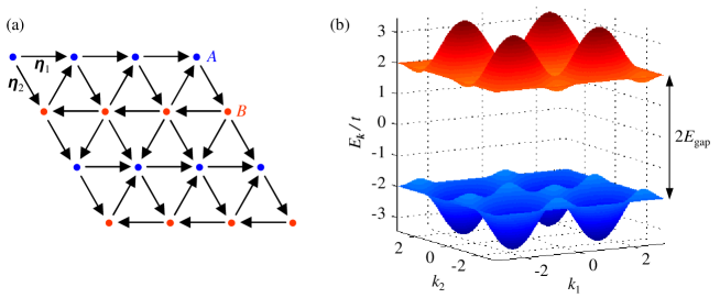
Figure 1: (a) One possible gauge of the tight-binding model of MFs on a triangular lattice, which is expressed in equation (2). An arrow from site $i$ to site $j$ means $s_{ij}=1$. Note that the lattice is split into two sublattices $A$ and $B$, and that the counterclockwise product of the $s_{ij}$’s around each triangle equals to $-1$. (b) The corresponding gapped spectrum, with $E_{\mathrm{gap}}=1.73$.

In particular, in the triangular lattice each plaquette encloses a quarter of flux quantum, and the product of the hopping terms equals $\mathrm{i}t^{3}$, revealing a time-reversal anti-symmetry. Moreover, the unit cell which encloses a flux quantum is a parallelogram of four neighboring triangles, leading to the lattice being composed of two sublattices. One possible gauge is illustrated in figure 1(a), which also depicts the two sublattices $A$ and $B$. In this gauge

$$H =\mathrm{i}t\sum_{i}\left(-\gamma_{A,i}\gamma_{A,i+\bm{\eta}_{1}}+\gamma_{B,i}\gamma_{B,i+\bm{\eta}_{1}}+\gamma_{B,i}\gamma_{A,i-\bm{\eta}_{2}}\right.$$ (2)

$$\qquad\qquad\left.+\gamma_{A,i}\gamma_{B,i-\bm{\eta}_{2}}-\gamma_{B,i}\gamma_{A,i+\bm{\eta}_{1}-\bm{\eta}_{2}}+\gamma_{A,i}\gamma_{B,i+\bm{\eta}_{1}-\bm{\eta}_{2}}\right).$$

Let us assume a clean periodic lattice of $L_{1}\times L_{2}$ sites, with $L_{2}$ even. We can define the Fourier transform $\bar{\Gamma}_{a,\bm{k}}=\sum_{i}\mathrm{e}^{-\mathrm{i}\bm{k}\bm{x}_{i}}\gamma_{a,i}$, where $a=A,B$ and $\bm{k}=2\pi(m_{1}/L_{1},m_{2}/2L_{2})$ for $m_{i}=0,...,L_{i}-1$ ($i=1,2$) [20]. These transformed operators are complex fermions, which satisfy $\{\bar{\Gamma}_{a,\bm{k}},\bar{\Gamma}_{a,\bm{k}^{\prime}}^{\dagger}\}=\delta_{\bm{k}\bm{k}^{\prime}}$. Note, however, that for $\bm{k}=(0,0)$, $(\pi,0)$, $(0,\pi/2)$ and $(\pi,\pi/2)$ they are MFs. By denoting spinor $\bar{\bm{\Gamma}}_{\bm{k}}^{\dagger}=(\bar{\Gamma}_{A,\bm{k}}^{\dagger},\bar{\Gamma}_{B,\bm{k}}^{\dagger})$ the Hamiltonian can be expressed as

$$H=2t\sum_{\bm{k}}\bar{\bm{\Gamma}}_{\bm{k}}^{\dagger}\left(\sin k_{2}\sigma_{x}-\cos(k_{1}-k_{2})\sigma_{y}-\sin k_{1}\sigma_{z}\right)\bar{\bm{\Gamma}}_{\bm{k}},$$ (3)

where the Pauli matrices act on the sublattice space. The resulting spectrum has an energy gap of $2tE_{\mathrm{gap}}$, where $E_{\mathrm{gap}}=1.73$, as depicted in figure 1(b).

The hopping elements between neighboring MFs are very sensitive to the inter-vortex separation. For example it was shown that for a $p_{x}\!+\!ip_{y}$ superconductor [23]:

$$t\sim\cos\left(k_{\mathrm{F}}r+{\pi\over 4}\right)\mathrm{e}^{-r/\xi},$$ (4)

where $k_{\mathrm{F}}$ is the Fermi momentum, $r$ is the inter-vortex distance, and $\xi$ is the coherence length, which is usually larger than $k_{\mathrm{F}}$. The exponential decay and the oscillations were found to occur also for the $\nu=5/2$ case [24], and are likely to appear in all realizations. Therefore small deformations of the Abrikosov lattice of order $k_{\mathrm{F}}^{\phantom{f}-1}$ will produce fluctuations in both the amplitude and sign of the hopping terms $t_{ij}$.

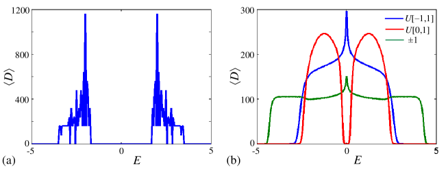
Figure 2: The disorder-averaged DOS $\langle D\rangle$ as a function of the energy $E$ of a periodic $30\times 30$ lattice with (a) uniform and (b) random hopping terms. In systems with hopping terms that are random both in sign and in magnitude (blue) and in systems where only the signs are random (green) there is a sharp peak at zero energy, while random amplitudes (red) only smear the spectrum of the clean system, but do not close the gap. The DOS is averaged over 10,000 realizations.

We find numerically that random hopping terms $t_{ij}=ts_{ij}$, where $s_{ij}$ is uniformly distributed in the interval $[-1,1]$, close the energy gap of the uniform system. The DOS, which appears in figure 2, shows that not only the gap is closed, but a peak emerges at zero energy. We can distinguish between random amplitudes and random signs of the hopping terms, i.e. $|s_{ij}|\sim U[0,1]$ or $s_{ij}=\pm 1$ in equal probability, respectively. The DOS of these two cases, which are also depicted in figure 2, clearly shows that the zero-energy peak in the DOS appears only due to random signs, while random amplitudes merely smear the spectrum without closing the energy gap. We are mostly interested in the zero-energy peak of the DOS, and therefore in the following we will focus on the case where disorder appears in the sign of the hopping terms.

The sharp peak that we found numerically for the density of states of finite systems close to zero-energy naturally raises the question of the way the DOS scales with the size of the system in the thermodynamic limit. Increasing the system size $L$ obviously increases the DOS. If the lowest energies decay faster than $1/L^{2}$, then the zero-energy DOS will increase faster than $L^{2}$, and the zero-energy DOS per unit area would diverge in the thermodynamic limit. Figure 3(a) exhibits the energy of the three lowest states $E_{1},E_{2}$ and $E_{3}$, averaged over disorder, as a function of the system size. In the given range a fit to $\langle E_{n}\rangle\propto 1/L^{\alpha}$ yields $\alpha\approx 2.18$ for $n=1,2$ and $3$, which indicates either a weak power-law or logarithmic divergence of the DOS per unit area.

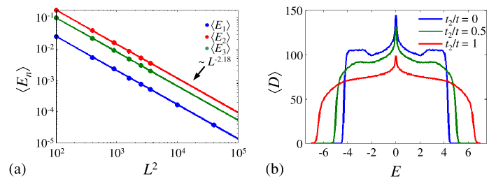
Figure 3: (a) The dependence of the disorder-averaged energies of the three lowest states $E_{1},E_{2}$ and $E_{3}$, as a function of the system size $L^{2}$, on a log-log scale. The energies $\langle E_{n}\rangle$ were averaged over 1000 realizations. Linear fitting gives $\langle E_{n}\rangle\propto L^{-2.18}$ for all three energies. (b) The disorder-averaged DOS $\langle D(E)\rangle$ with first ($t$) and second ($t_{2}$) nearest neighbors hopping, both with random signs, for $t_{2}/t=0,0.5,1$. As $t_{2}$ approaches $t$ the DOS approaches a semicircle. The DOS is of a $30\times 30$ lattice, and was averaged over 1000 realizations.

It is instructive to compare the DOS we find for the case of random nearest-neighbor hopping to that we find for the case of a random Hermitian matrix of imaginary terms. The DOS of the latter is a version of a semicircle distribution, with a Delta peak at zero energy, due to the symmetry of the spectrum with respect to reflection about zero energy [25]. When we add second nearest-neighbor hopping with random signs to the Hamiltonian, the DOS indeed gets closer to the semicircle. Figure 3(b) shows the spectrum for several ratios of $t_{2}$, the amplitude of the next-nearest-neighbor terms, to $t$. We note, however, that we numerically find the gap to close even for the clean system when $t_{2}/t\approx 0.58$.

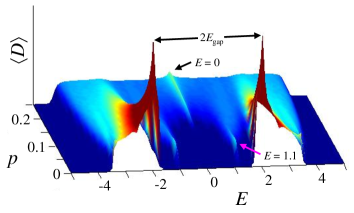
Figure 4: The disorder-averaged DOS $\langle D(E)\rangle$ of a periodic $70\times 70$ lattice as a function of the probability $p$ for flipping the sign of a hopping term. For $p=0$ the DOS is that of figure 2(a). Two small peaks at $E\approx\pm 1$, that grow linearly with $p$, belong to localized states which are created around a single isolated flipped hopping term. The zero-energy peak grows slowly, but survive at the disordered system. The DOS is averaged over 100 realizations.

Having established that the DOS of the clean lattice is characterized by an energy gap limited by two singular peaks, and the lattice where the sign of the hopping terms is random is characterized by a zero energy peak above a gapless background, we examine the evolution of the DOS with $p$, the probability of flipping the sign of a hopping term, which increases from 0 (the clean lattice) to 0.5 (the random sign limit). Figure 4(a) shows how increasing $p$ makes the singular peaks of the clean system spread, and gradually creates sub-gap states.

In the next section we study the way the gap is closed, and especially the appearance of the zero-energy peak. We address these questions by an examination of two limits. In the weak disorder limit, we present the minimal disorder configuration that results in a zero-energy state. In the strong disorder limit, we examine the low-energy states that are formed along domain walls between regions in which the signs of flux piercing the plaquettes are opposite.

3 The origin of the zero-energy peak in the density of states

We have seen that the clean triangular lattice of MFs is anti-symmetric under time reversal, and has an energy gap. Depending on the sign of the hopping tunneling elements, the MFs may be mapped onto electrons in a triangular lattice pierced by $1/4$ or $-1/4$ flux quanta per plaquette. These two cases are characterized by two opposite Chern numbers: by writing the $k^{th}$ component of equation (3) as $H_{k}=2t\bm{h}_{\bm{k}}\cdot\bm{\sigma}$, it is easy to see that the Majorana band is characterized by a non-trivial Chern number

$$\nu = \mathrm{sign}(t)\int\frac{\mathrm{d}^{2}k}{4\pi}\frac{1}{|\bm{h}_{\bm{k}}|^{3}}\left(\bm{h}_{\bm{k}}\cdot\frac{\partial\bm{h}_{\bm{k}}}{\partial k_{1}}\times\frac{\partial\bm{h}_{\bm{k}}}{\partial k_{2}}\right)$$ (5)

$$= \mathrm{sign}(t)\int_{-\pi}^{\pi}\mathrm{d}k_{1}\int_{-\pi/2}^{\pi/2}\mathrm{d}k_{2}\frac{\sin^{2}(k_{1}-k_{2})+\cos k_{1}\cos k_{2}\cos(k_{1}-k_{2})}{4\pi\left[\sin^{2}k_{1}+\sin^{2}k_{2}+\cos^{2}(k_{1}-k_{2})\right]^{3/2}}$$

$$= \mathrm{sign}(t).$$

The disorder-induced reversal of signs of hopping terms may revert the sign of the flux in some of the plaquettes in the lattice. The systems would then have islands of one phase separated by lines of interface from the bulk of the other phase. An infinite interface between two phases of different Chern numbers is accompanied by gapless modes [26, 27, 28]. For finite islands, one may naively expect finite-size quantization to induce a gap in the energy spectrum, and thus low-energy excitations to require large islands. This expectation is only partially valid. As we explain below, for the Majorana lattice, large islands are associated with low-energy excitations at their edges, but small islands may carry low-energy and zero-energy modes as well.

When the probability $p$ of flipping the sign of a hopping term is very small the flipped terms are dilute, and most of them are isolated. A two-triangles island, which is created by flipping the sign of a single hopping term, results in two localized sub-gap states with energies of approximately $\pm 1.1$. Theses states are the source of the peaks in the DOS at $\pm E\approx\pm 1.1$, and indeed in the limit of small probability the DOS associated with these peaks $\langle D(E\approx\pm 1.1)\rangle\propto p$. Such islands do not, however, contribute to the DOS close to zero energy.

As we show in A, flipping three hopping terms with a common vertex creates two localized states with energy that is either zero or exponentially small with the system size. We also show that this is the minimal way of creating zero modes. Thus, for small $p$ the zero-energy DOS is dominated by the probability of creating such configurations, and should scale like $p^{3}$. The two modes are, however, split when there is a single flipped hopping term at a distance $r$ from that vertex. The exact splitting depends on the orientations of the bonds with flipped signs, but we found numerically that it can be well approximated by $\pm E_{\mathrm{t}}(r)\approx\pm 6\mathrm{e}^{-2r}$. For $E_{\mathrm{t}}$ to be much smaller than the typical finite-size energy splitting, that scales as $L^{-2}$, we need $r\gg\log{L}$. A given radius $r$ encloses approximately $3\pi r^{2}$ hopping terms around the vertex, and the probability that all these terms are unflipped is $(1-p)^{3\pi r^{2}}$. Thus, the $p^{3}$ dependence of the zero-energy DOS is limited to small values of $p\ll\log^{-2}L$. For example, for a $70\times 70$ lattice we get $p<0.01$.

As $p$ gets large, the plaquettes in which the flux is reversed connect to one another, and the system is split into domains with opposite fluxes. To understand the excitations spectrum in this limit, we first examine the spectrum of excitations associated with the various possible interfaces of two large domains of opposite fluxes. Then, we examine the statistical distribution of such interfaces as a function of the flipping probability $p$.

At the interface between a macroscopic region of Chern number $\nu=\pm 1$ and the vacuum, a chiral gapless mode must appear [26, 27, 28]. In order to explicitly find this mode, we first replace $\bm{\eta}_{1}$ and $\bm{\eta}_{2}$ in equation (2) by $\hat{x}$ and $\hat{y}$ for simplicity, and denote the lattice sites by $\bm{x}$. We assume rotational symmetry along $\hat{y}$, and define the operators $\Gamma_{a,kx}=\sum_{y}\mathrm{e}^{-\mathrm{i}ky}\gamma_{a,\bm{x}}$ with $a=A,B$ and $k=\pi m/L_{y}$, where $m=0,...,L_{y}-1$. Each $\Gamma_{a,kx}$ represents a wavefunction that is localized at $\hat{x}$ but extended at $\hat{y}$. With these operators the Hamiltonian becomes

$$H=-t\sum_{k,x}\left[\bm{\Gamma}_{k,x}^{\dagger}(\mathrm{e}^{-\mathrm{i}k}\sigma_{y}+\mathrm{i}\sigma_{z})\bm{\Gamma}_{k,x+1}+\bm{\Gamma}_{k,x}^{\dagger}(\mathrm{e}^{\mathrm{i}k}\sigma_{y}-\mathrm{i}\sigma_{z})\bm{\Gamma}_{k,x-1}-\bm{\Gamma}_{k,x}^{\dagger}(2\sin k\sigma_{x})\bm{\Gamma}_{k,x}\right].$$ (6)

Given a right edge at $x=0$, the edge eigenmode of (6) for $x\leq 0$ is $\sum_{n=0}^{\infty}b_{k}^{\phantom{k}-2n}(1,1)\bm{\Gamma}_{k,-2n}$, where $b_{k}=\mathrm{i}\mathrm{e}^{-\mathrm{i}k}\tan(k/2)\approx\mathrm{i}{1\over 2}k\ll 1$ and $(a,b)\bm{\Gamma}_{k,x}=a\Gamma_{A,k,x}+b\Gamma_{B,k,x}$. For $k=0$ it reduces to $(1,1)\bm{\Gamma}_{0,0}$. The dispersion of the edge mode is $E_{k}=2\sin k$, with $E_{k}\approx 2k=2\pi m/L_{y}$ at low energy. Note that the wavefunction is localized in the $\hat{x}$ direction with a localization length of the order of $1/\log(L_{y}/\pi m)\sim 1/\log{E}$, which depends weakly on the energy and the system size.

A triangular lattice with one periodic coordinate can have either flat or zigzag edges, depending on the way the periodic boundary condition is taken, as illustrated in figure 5. The Hamiltonian (6) describes a flat edge. In a zigzag edge, we also get a chiral edge mode, with the dispersion $E_{k}\approx\sqrt{2}k$ and $b_{k}\approx(3-2\sqrt{2})-(8-11/\sqrt{2})k^{2}$, which gives a localization length that is approximately independent of energy, at low energies. We can see that in spite of the differences, both edges show a similar behavior of linear dispersion and exponentially localized wavefunction. Henceforth we will assume the periodicity of equation (6).

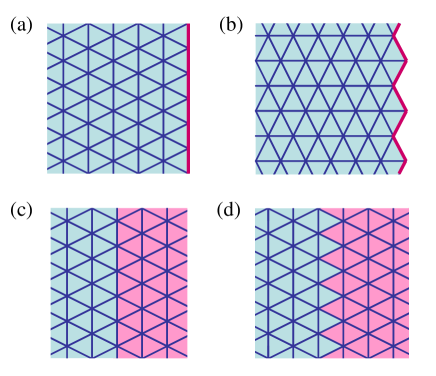
Figure 5: Two types of edges in the triangular lattice with one periodic coordinate: (a) flat and (b) zigzag. With the periodic coordinate of (a) there are two types of domain walls between P-phase (azure) and N-phase (pink) that preserve the translational symmetry: (c) flat and (d) sawtooth.

An interface, or domain wall, between the two phases of opposite Chern numbers is expected to hold two chiral edge modes, similar to the single mode that exists along the interface between any of the two phases and the vacuum. We denote the unflipped phase by P and the flipped phase by N, representing their positive and negative fluxes respectively. A periodic lattice with an interface between a P-phase and an N-phase may have two kinds of domain walls that preserve the translational symmetry: flat and sawtooth, as depicted in figure 5.

A flat domain wall is created when $\sigma_{y}\rightarrow-\sigma_{y}$ in the hopping terms for $x>0$. The two chiral modes of such a domain wall have the same dispersion and amplitudes $b_{k}$ as the flat edge mode, where in the N-phase the amplitudes are $b_{k}^{\phantom{k}*}$, as expected from the time reversal. Only now one mode has non-vanishing amplitudes at $x=2n$, while the other mode has non-vanishing amplitudes at $x=2n+1$. A sawtooth domain wall is a result of flipping the $\sigma_{x}$’s. It shows essentially a similar behavior to the flat domain wall, but with $E_{k}\approx 1.95(k\pm k_{\mathrm{z}})$, where $k_{\mathrm{z}}=\arccos(\sqrt{5}/2-1/2)$. Again, we see that the geometry of the domain walls has only a small effect on the low-energy physics.

If an ‘island’ of a roughly circular shape of the N-phase is surrounded by the P-phase lattice, then the two chiral modes will be localized along the perimeter of the island, and their dispersion will be $E_{m}\sim m/M$, where $M$ is the perimeter of the island. Such an island will close the energy gap only if it becomes macroscopic.

In a disordered system where the sign of the hopping term $s_{ij}$ is random, islands of the N-phase will be created in various shapes and sizes. A way to parameterize the morphology of an island is by the perimeter-area relation. In approximately rounded shapes $M\propto A^{1/2}$, where $A$ is the area of the island, while in a narrow strip $M\propto A$. Figure 6(a) depicts the distribution of the perimeters as a function of the areas of random islands in a $30\times 30$ lattice, where the probability of flipping a sign is $1/2$. The area of an island is the number of N-triangles that compose the island, where two N-triangles are defined to belong to the same island if they share at least a vertex. The perimeter is composed of the P-triangles which have a common vertex with the island. For islands with $A>10$ the mean perimeter can be excellently approximated by $\langle M(A)\rangle\approx 2.34A+15.6$, which means that the islands look like snakes or gossamer.

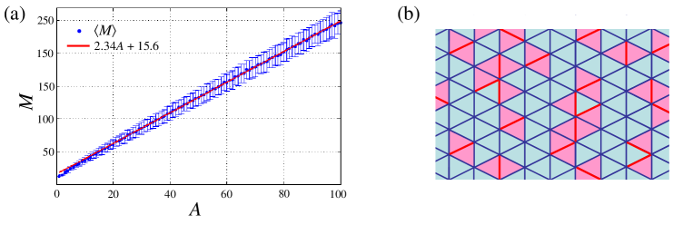
Figure 6: (a) The distribution of the perimeters $M$ of the N-phase islands with a given area $A$, where the islands were created by hopping terms with random signs. The error bars are located at the mean values $\langle M\rangle$, with the width of a standard deviation. The mean value is excellently fitted to a linear curve (red line). The distribution was taken from 10,000 random realizations of a $30\times 30$ lattice. (b) A typical islands configuration of N-triangles (pink) that are created by random flipping of hopping terms (red), with a complicated geometry of rhombi and triangles. In this realization 0.14 of the hopping terms are flipped.

The smallest island that may be created by flipping the sign of a single hopping term is composed of two triangles, and has a rhombus shape. The simplicity of the shapes is not preserved for larger islands. Flipping two neighboring hopping terms results in two flipped N-triangles, but those share only a vertex. Larger islands are typically of complicated shapes, composed of rhombi and triangles, as illustrated in figure 6(b). Complicated islands provide complicated dispersion and DOS, as we will demonstrate. In order to get a feeling to the resulting dispersions, we now focus on three types of narrow islands that preserve the translational symmetry, i.e. strips of N-triangles.

The method we use for approximating the low-energy dispersion of the strips is first to find zero-energy modes with $k=0$, and then extract the dominant $k$-dependence employing first order perturbation theory. For the clean system the Hamiltonian (6) may be recast as

$$H = H_{0}+\sum_{k\neq 0}\delta H_{k},$$ (7a)

$$H_{0} = 2t\sum_{x}\bm{\Gamma}_{0,x}(-\sigma_{y}+\mathrm{i}\sigma_{z})\bm{\Gamma}_{0,x+1},$$ (7b)

$$\delta H_{k} = 2t\sin{k\over 2}\sum_{x}\left(\mathrm{e}^{-\mathrm{i}k/2}\bm{\Gamma}_{k,x}^{\dagger}\mathrm{i}\sigma_{y}\bm{\Gamma}_{k,x+1}-\mathrm{e}^{\mathrm{i}k/2}\bm{\Gamma}_{k,x}^{\dagger}\mathrm{i}\sigma_{y}\bm{\Gamma}_{k,x-1}+2\cos{k\over 2}\bm{\Gamma}_{k,x}^{\dagger}\sigma_{x}\bm{\Gamma}_{k,x}\right).$$ (7c)

For any strip $\mathrm{s}$, this Hamiltonian has to be modified to the Hamiltonian $H^{\mathrm{s}}$, which may be decomposed similarly to $H_{0}^{\mathrm{s}}$ and $\delta H_{k}^{\mathrm{s}}$. The $k=0$ zero modes of $H^{\mathrm{s}}$ will be denoted by $\Gamma^{\mathrm{s}}_{i}=\Gamma^{\mathrm{s}{\dagger}}_{i}$. They satisfy $[H_{0}^{s},\Gamma^{\mathrm{s}}_{i}]=0$. In the cases we will explicitly consider here, there are two zero modes per strip. The matrix elements of $\delta H_{k}$ between these zero modes give the leading order of the $k$-dependence. Therefore after finding $\Gamma^{\mathrm{s}}_{\mathrm{I}}$ and $\Gamma^{\mathrm{s}}_{\mathrm{II}}$, we diagonalize the matrix $[\delta H_{k}]$, where $[\delta H_{k}]_{ij}=\{\Gamma^{\mathrm{z}}_{i},[\delta H_{k},\Gamma^{\mathrm{z}}_{j}]\}$

The first and simplest strip is the flat strip, which is depicted in figure 7(a), and is created by flipping the sign of the $\sigma_{z}$’s in equation (7b) between $x=0$ and $x=1$. Now $H_{0}^{\mathrm{flat}}$ has two zero modes:

$$\Gamma_{\mathrm{I}}^{\mathrm{flat}} = {1\over\sqrt{2}}(1,1)\bm{\Gamma}_{0,0},$$

$$\Gamma_{\mathrm{II}}^{\mathrm{flat}} = {1\over\sqrt{2}}(1,-1)\bm{\Gamma}_{0,1}.$$ (7h)

The matrix elements of $\delta H_{k}$ in the zero modes space are

$$[\delta H_{k}]^{\mathrm{flat}}=-t\sin{k}\left(1,-\tan{k\over 2},2\right)\cdot\bm{\tau},$$ (7i)

with $\bm{\tau}$ being the vector of Pauli matrices. The resulting corrections to the zero energies are $\delta E_{k}^{\mathrm{flat}}\approx\pm\sqrt{5}tk$. These modes are essentially the domain wall modes, which are modified due to their hybridization, and similarly their DOS is a constant.

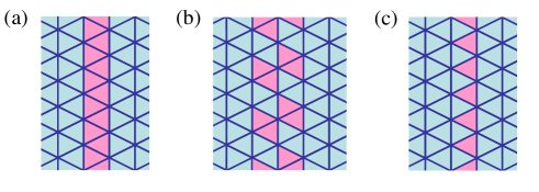
Figure 7: The three examples of narrow islands of N-phase, whose chiral sub-gap modes show three kinds of dispersion: (a) a flat strip with $E_{k}\propto k$, (b) a ‘zipper’ strip with $E_{k}\propto k^{2}$ and (c) a sawtooth strip with $E_{k}\propto k^{3}$.

The second example is a ‘zipper’ strip, shown in figure 7(b), which is a result of replacing $\sigma_{y}$ of Equations (7b) and (7c) by $\mathrm{i}\sigma_{x}$ for $x=-1$ and by $-\mathrm{i}\sigma_{x}$ for $x=0$. Two zero modes again appear

$$\Gamma_{\mathrm{I}}^{\mathrm{zip}} = \frac{1}{2\sqrt{2}}\left[(1,1)\bm{\Gamma}_{0,-2}+(0,2)\bm{\Gamma}_{0,0}-(1,-1)\bm{\Gamma}_{0,2}\right],$$

$$\Gamma_{\mathrm{II}}^{\mathrm{zip}} = {1\over 2}\left[(1,1)\bm{\Gamma}_{0,-1}+(1,-1)\bm{\Gamma}_{0,1}\right],$$ (7j)

which yields $[\delta H_{k}]^{\mathrm{zip}}=-\sqrt{2}t\sin^{2}{k\over 2}\sigma_{y}$. The corrections to the energies are now quadratic $\delta E_{k}^{\mathrm{zip}}\approx\pm{1\over\sqrt{8}}tk^{2}$. Note that these modes are wider, and that their DOS diverge as $E^{-1/2}$.

The third example is the sawtooth strip, which is created by multiplying the hopping terms between $x=-1$ and $x=0$ by $\sigma_{z}$, and is shown in figure 7(c). The zero modes are now

$$\Gamma_{\mathrm{I}}^{\mathrm{saw}}={1\over\sqrt{2}}(1,-1)\bm{\Gamma}_{0,0},$$

$$\Gamma_{\mathrm{II}}^{\mathrm{saw}}={1\over 2}\left[(1,1)\bm{\Gamma}_{0,-1}+(1,-1)\bm{\Gamma}_{0,1}\right].$$ (7k)

Unfortunately, $[\delta H_{k}]^{\mathrm{saw}}=-t(1+\tau_{z})\sin{k}$, which means that the first order perturbation theory gives the correction only to the first mode $\delta E_{k}^{\mathrm{saw}}\approx-2tk$, while the second mode requires higher orders. An explicit solution of this mode gives $\delta E_{k}^{\mathrm{saw}}\approx k^{3}$; thus this soft mode makes the DOS diverge as $E^{-2/3}$.

We can conclude from this section that along edges and domain walls chiral modes appear with linear low-energy dispersion. These modes close the energy gap only for macroscopic domain walls, which will give a constant DOS. However, when the domains become narrow strips, the dispersions of the chiral modes strongly depend on the geometry of the strip, and their DOS tends to diverge at zero energy. And since most domains which are created by random hopping terms are composed of narrow strips, this may explain the zero-energy peak raising above the uniform background in the DOS.

4 Percolation phase transition

In the previous section we have seen that chiral modes which are localized along stripe-shaped domains may lead to a zero-energy peak in the DOS when the signs of the hopping terms are random. Such modes provide low-energy states (states whose energy scales inversely with the size of the system) only if the length of the domain is of the order of the system size. For hopping terms whose signs are random ($p=0.5$) there are such extended domains, since triangles of both phases are distributed all over the lattice. In contrast, for small $p$ only small isolated domains are created.

In this section we address the dependence of the DOS on $p$. We start by examining the dependence of the size of the islands on $p$. It is natural to expect a percolation phase transition, where below a critical probability $p_{\mathrm{c}}$ only microscopic islands can be found in the lattice. The probability distribution to find an island with area $A$ is then exponential with $A$, where the typical area depends on $p$ and is independent of the system size $L$. Above $p_{\mathrm{c}}$ a macroscopic island forms; thus the probability distribution is concentrated around the macroscopic value, which of course scales as $L^{2}$.

This expectation is borne out by our numerical analysis. Figure 8 depicts the distribution of the islands area $A$, normalized to the system’s size $L^{2}$, as a function of $p$ for an $L=100$ lattice. For large $p$ the distribution appears to be concentrated around a mean value, which was numerically verified to scale as $L^{2}$. In contrast, for small $p$ the distribution is approximately exponential in a manner that was found to be independent of $L$. The transition takes place at $p_{\mathrm{c}}\approx 0.15$. The width of the transition between the microscopic and macroscopic distributions, which takes place here in $0.10<p<0.15$, gets sharper towards $p_{\mathrm{c}}$ while increasing $L$.

Since flipping a hopping term flips the fluxes of two triangles, islands with even values of $A$ are more common than islands with odd values of $A$. Figure 8 shows that in spite of the different distribution of the even and odd values of $A$, both are exponentially distributed below $p_{\mathrm{c}}$.

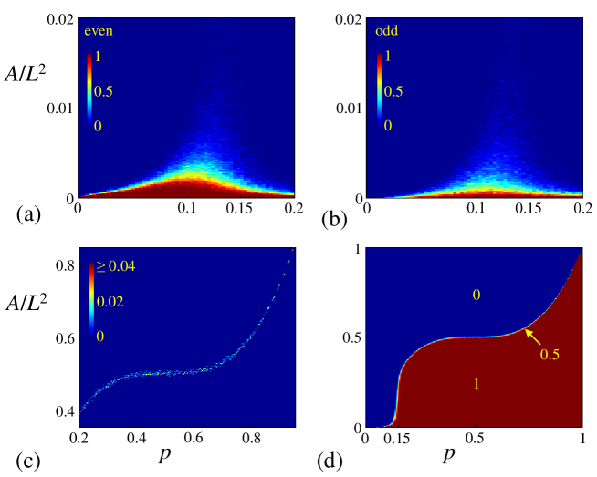
Figure 8: The distribution of the normalized area $A/L^{2}$ of the N islands as a function of the probability of flipping a hopping term $p$ for a $100\times 100$ lattice. (a,b) The probability of having an island with area $A/L^{2}$ for small $p$. The probability is approximately exponentially distributed, in both even and odd values of $A$, regardless of the system size. This means that for small $p$ in every realization there are many microscopic islands. (c) For large $p$ the probability is concentrated around a mean macroscopic value, i.e. there is a single macro-island. (d) The probability of having an island with area larger than $A/L^{2}$ as a function of $p$. The curve of probability 0.5 indicates the characteristic largest island. The vertical slope at $p_{\mathrm{c}}\approx 0.15$ indicates a percolation phase transition. The distribution was built upon 100 realizations.

Figure 8(d) depicts, for every $p$ and normalized area $A/L^{2}$, the probability that there are islands larger in area than $A/L^{2}$. The curve for which this probability is $0.5$ is the typical size of the largest island for a particular disorder realization. We denote this curve by $A_{\mathrm{max}}(p)$. If we measure the flux in the system with reference to the flux of the clean system, then since a triangle with N flux is formed by flipping either one or all three hopping terms forming the triangle, the mean flux threading the lattice is $\langle\phi\rangle=2L^{2}[3p(1-p)^{2}+p^{3}]$. Above $p_{\mathrm{c}}$ the macroscopic island, if it exists, is supposed to capture almost all the N flux. Indeed, $A_{\mathrm{max}}(p>p_{\mathrm{c}})$ is excellently approximated by $\langle\phi\rangle$. Thus, above $p_{\mathrm{c}}$ almost all the triangles with flipped flux are connected.

Figure 9 depicts two low-energy disorder-averaged quantities for various lattice sizes $L$. The first is $\langle E_{1}(p)\rangle$, the energy of the lowest excitation. The second is the zero-energy DOS $\langle D_{0}\rangle$, which we define as the number of states within the energy window $0\leq E<E_{\mathrm{sat}}$, divided by $E_{\mathrm{sat}}$, where $E_{\mathrm{sat}}=\langle E_{1}(p\rightarrow 0.5)\rangle$ is the disorder averaged energy of the lowest excitation for the $p=0.5$ case, extracted from figure 3. In order to compare systems with different sizes, we normalize $\langle E_{1}(p)\rangle$ by $E_{\mathrm{sat}}(L)$, and $\langle D_{0}\rangle$ by $D_{\mathrm{sat}}=\langle D_{0}(p\rightarrow 0.5)\rangle$.

For small $p$ we find $\langle E_{1}\rangle$ to approach the value of the energy gap, as it should. We find $\langle D_{0}\rangle$ to be polynomial in $p$ for small $p$, in accordance with our estimate for the probability of finding isolated regions of zero-energy states. Above the percolation phase transition the mean minimal energy $\langle E_{1}\rangle$ and the zero-energy DOS $\langle D_{0}\rangle$ are expected to saturate to a constant value as a function of $p$. We do indeed observe a saturation of $\langle E_{1}\rangle$ and $\langle D_{0}\rangle$ above $p_{c}$.

Surprisingly, figure 9(a) shows that the approach to the saturated value is not monotonic. The minimal $\langle E_{1}\rangle$ appears at $p_{\mathrm{e}}\approx 0.11<p_{\mathrm{c}}$, and we find $\langle E_{1}(p_{\mathrm{e}})\rangle\propto L^{-2.88}$, as shown in figure 9(c). Moreover, the maximum $\langle D_{0}\rangle$ also appear at $p_{\mathrm{e}}$. The divergence of the DOS at zero energy seems therefore to be strongest before the percolation threshold.

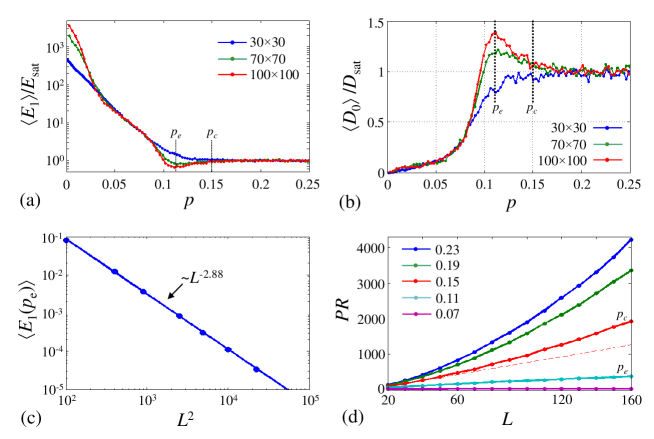
Figure 9: (a) The normalized mean minimal energy $\langle E_{1}\rangle/E_{\mathrm{sat}}$ as a function of the probability $p$, where $E_{\mathrm{sat}}=\langle E_{1}(p\rightarrow 0.5)\rangle$. The percolation phase transition is manifested as the saturation to constant values for $p>p_{\mathrm{c}}$, but surprisingly the lowest energies appear around $p_{\mathrm{e}}<p_{\mathrm{c}}$, which means that they belong to localized states. (b) The mean zero-energy DOS $\langle D_{0}\rangle=\langle D(0\leq E<E_{\mathrm{sat}})\rangle$ as a function of $p$, normalized by its value at $p=0.5$, $D_{\mathrm{sat}}$, of the same lattices. The saturation for $p>p_{\mathrm{c}}$ is expected, but the DOS gets its maximal values at $p_{\mathrm{e}}<p_{\mathrm{c}}$, and decays towards zero only in a polynomial manner. (c) The mean minimal energy at $p_{\mathrm{e}}$ as a function of the system size is very well fitted to $L^{-2.88}$. (d) The disorder-averaged participation ratio $PR$ of the minimal energy state as a function of the system size $L$, for various values of $p$. For $p>p_{\mathrm{c}}$ the state is extended, since $PR$ scales faster than $L$ (denoted by dashed line). For $p\ll p_{\mathrm{c}}$ the states are localized, since $PR$ is independent of $L$. At $p\approx p_{\mathrm{e}}$, $PR\sim L$, which implies a 1D string-like state.

If the percolation phase transition captures the essence of the low-energy physics, we naively expect the low-energy states to be extended above $p_{\mathrm{c}}$, while those below $p_{\mathrm{c}}$, including $p_{\mathrm{e}}$, to be localized. For any eigenstate of the Hamiltonian $\Gamma_{E}=\sum_{i}a_{i}\gamma_{i}$, the localization properties of the state can be characterized by the participation ratio (PR), defined by $PR=(\sum_{i}|a_{i}|^{4})^{-1}$. The PR of a perfect metal scales linearly with the system size $L^{2}$, while the PR of an insulator is independent of $L$. Figure 9(d) depicts the disorder-averaged PR of the lowest excitation as a function of the system size, for various values of $p$. As expected, above $p_{\mathrm{c}}$ the PR scales faster than $L$, which indicates an extended state, while well below $p_{\mathrm{c}}$ the PR is independent on $L$. However, at $p_{\mathrm{e}}$ the PR scales as $L$. This scaling seems to imply that there is a range of $p$ in which the low-energy states are string-like in the sense that they are macroscopic only along one dimension. Recalling the observed diverging DOS of the edge states along the narrow strips, the divergence of $\langle D_{0}\rangle$ at $p_{\mathrm{e}}$ is understood, even if not the precise exponent.

5 Summary

In the previous sections we have seen that the zero-energy peak of the DOS for random signs in the nearest neighbor hopping terms may have different sources in two limits of the probability $p$ for flipping the sign of individual hopping terms. For small $p$ the peak is the consequence of the existence of localized zero-energy states and the tunneling between them and other localized states. Therefore it appears on a background of the zero DOS of the energy gap, and it is proportional to $p^{3}$. In the opposite limit of $p_{\mathrm{c}}\leq p\leq 0.5$, where $p_{\mathrm{c}}\approx 0.15$, macroscopic islands of the time-reversed phase cross the lattice, and the gap is closed due to the low-energy modes along the interfaces of these islands with the original phase. Since the dispersion of some of these modes is nonlinear, they are expected to create zero-energy peak in the DOS. Our numerical results indicate a weak divergence of the DOS at zero energy for $p=0.5$, and an even stronger divergence somewhat below the percolation transition. In this region the islands seem to be of the form of strings, and the mentioned nonlinear dispersion is likely to be the source the divergence.

It was mentioned above that the Hamiltonian of our system is purely imaginary and anti-symmetric both to charge conjugation and time-reversal. According to the standard classification of disordered Hamiltonians [29] it belongs to class D [30, 31]. This class is known to have three distinct phases: thermal metal, thermal insulator and thermal quantum Hall (TQH) insulator [32, 33]. In the metal phase, the DOS at zero energy diverges logarithmically with the system size [32]. Several numerical studies of the properties of this class have been carried out using the Cho-Fisher network model [34, 35, 36], which exhibits all of the phase diagram. It was found that in the TQH phase there is a region below the insulator-metal transition where the DOS at zero energy diverges, but with a nonuniversal exponent, due to the effects of rare configurations of disorder (Griffiths phase) [36]. Recently a model of MFs on a square lattice created in a $p$-wave superconductor by a random potential has been proposed [10], and the divergence in the metal phase has also been observed numerically there.

Our model is a new realization to the TQH–thermal metal transition, which may be physically realizable. We observe the divergence of the DOS both in the metal regime and in the analogue to the Griffiths regime, and the microscopic understanding of our system provides insights into the physics of these phenomena.

Note added: After completing the preparation of this manuscript, we became aware of a study of a similar system carried out by C Lohmann, AWW Ludwig and S Trebst [37].

Appendix A Minimal zero mode

In this appendix we prove that flipping three hopping terms with a common vertex in a periodic clean lattice results in two localized states with energy which is either zero or exponentially small with the system size. The proof also implies that there is no way to create zero modes with flipping less than three signs.

The hopping signs $s_{ij}$ in the Hamiltonian (1) define a matrix $S$, which is skew-symmetric $S^{T}=-S$, and therefore has a well defined Pfaffian. The recursive definition of the Pfaffian of an $N\times N$ matrix is

$$\mathrm{Pf}(A)=\sum_{i=1}^{N}(-1)^{i}a_{1i}\mathrm{Pf}(\hat{A}_{1i}),\\$$ (7l)

$$\mathrm{Pf}\left(\begin{array}[]{cc}0&a\\ -a&0\end{array}\right)=a\qquad\mathrm{Pf}(0)=0,$$

where $a_{ij}$ is the element $i,j$ of $A$, and $\hat{A}_{1i}$ is the matrix $A$ without the $1^{\mathrm{st}}$ and $i^{\mathrm{th}}$ rows and column. A useful property of the Pfaffian [39] is that for any matrix $B$

$$\mathrm{Pf}(BAB^{T})=\det(B)\cdot\mathrm{Pf}(A).$$ (7m)

The gauge transformation $\gamma_{i}\rightarrow-\gamma_{i}$ flips the signs of the $i^{\mathrm{th}}$ row and column of $S$. This transformation can be done by a diagonal matrix $B$ with the elements $b_{jj}=(-1)^{\delta_{ji}}$. And since $\det(B)=-1$, the gauge transformation flips the sign of $\mathrm{Pf}(S)$. Moreover, swapping labels of two sites, also flips the sign of $\mathrm{Pf}(S)$, since it can be performed by $B=I_{(N-2)\times(N-2)}\times\sigma_{x}$, where $\sigma_{x}$ is the Pauli matrix which acts in the space of the two swapped sites.

Systematic gauge transformations reveal equivalence relations between apparently different lattices. The simplest example is the gauge transformation that swaps between the two sublattices, which is depicted in figure 10(a). In a periodic lattice the number of rows is even (which means that the two sublattices are indeed equivalent), an even number of sites are gauged, and the Pfaffian is unchanged. Rotations by $60^{\circ}$ clockwise and counterclockwise can be also produced by gauge transformations, as depicted in figures 10(b) and 10(c). In principle, such rotations may multiply the Pfaffian by a factor of $-1$. However, three $60^{\circ}$ rotations result in swapped sublattices, which does not change the Pfaffian, and hence one rotation must leave the Pfaffian unchanged as well. Note that in finite lattices the $60^{\circ}$ rotations may have $O(\mathrm{e}^{-L})$ corrections, due to change of boundary conditions.

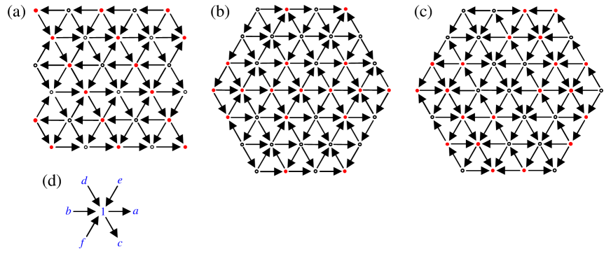
Figure 10: (a) The gauges transformation that swaps between the two sublattices. A red cycle means $\gamma_{i}\rightarrow-\gamma_{i}$; thus all the arrows connected to the site $i$ are flipped. (b,c) Gauge transformation which produce $60^{\circ}$ (b) clockwise and (c) anticlockwise rotations. (d) An arbitrary site is denoted by 1 and its six neighbors by $a$–$f$.

All these gauge-dependent properties of the Pfaffian show that it is an unphysical quantity. However, since $\mathrm{Pf}(A)^{2}=\det(A)$, the Hamiltonian $H$ has zero energy states iff $\mathrm{Pf}(S)=0$. Therefore the way to prove that flipping three neighboring arrows gives zero-energy states, would be to prove that the Pfaffian vanishes for such a configuration.

Let us denote an arbitrary lattice site by 1, and its six neighbors by $a,b,..,f$, as depicted in figure 10(d). According to definition (7l)

$$\mathrm{Pf}(S)=\sum_{i=a}^{f}(-1)^{i}s_{1i}\mathrm{Pf}(\hat{S}_{1i}).$$ (7n)

The physical meaning of $\mathrm{Pf}(\hat{S}_{1i})$ is omitting the sites 1 and $i$. We look for relations between lattices with vacancies of two neighboring sites. These relations will allow us to express five of the terms $\mathrm{Pf}(\hat{S}_{1i})$ in (7n) in terms of the sixth, say $\mathrm{Pf}(\hat{S}_{1a})$.

Due to the horizontal symmetry of our gauge, it is apparent that $|\mathrm{Pf}(\hat{S}_{1b})|=|\mathrm{Pf}(\hat{S}_{1a})|$, but since the labeling of the sites is different, they may differ in signs. If, however, we ‘push’ the $a^{\mathrm{th}}$ row and column of $\hat{S}_{1b}$ $a-b-1$ rows and columns upwards, we get exactly $\hat{S}_{1,a}$. This process involves $a-b-1$ labels swapping; thus $\mathrm{Pf}(\hat{S}_{1b})=(-1)^{a-b-1}\mathrm{Pf}(\hat{S}_{1a})$. $\hat{S}_{1c}$ and $\hat{S}_{1d}$ are related by swapping the two sublattices; thus $|\mathrm{Pf}(\hat{S}_{1d})|=|\mathrm{Pf}(\hat{S}_{1c})|$. By ‘pushing’ the row and columns, we get again $\mathrm{Pf}(\hat{S}_{1d})=(-1)^{c-d-1}\mathrm{Pf}(\hat{S}_{1c})$. In a similar manner we have $\mathrm{Pf}(\hat{S}_{1f})=(-1)^{e-f}\mathrm{Pf}(\hat{S}_{1e})$. Furthermore, $\hat{S}_{1c}$ ($\hat{S}_{1e}$) is related to $\hat{S}_{1a}$ by the anticlockwise (clockwise) rotation, hence $|\mathrm{Pf}(\hat{S}_{1e})|\approx|\mathrm{Pf}(\hat{S}_{1c})|\approx|\mathrm{Pf}(\hat{S}_{1a})|$. By counting the number of sites been gauges, we get $\mathrm{Pf}(\hat{S}_{1c})=(-1)^{a-c}\mathrm{Pf}(\hat{S}_{1a})+O(\mathrm{e}^{-L})$ and $\mathrm{Pf}(\hat{S}_{1e})=(-1)^{a-e-1}\mathrm{Pf}(\hat{S}_{1a})+O(\mathrm{e}^{-L})$. Substituting all these relations in equation (7n) yields

$$\mathrm{Pf}(S)=(-1)^{a}(s_{1a}-s_{1b}+s_{1c}-s_{1d}-s_{1e}-s_{1f})\mathrm{Pf}(\hat{S}_{1a})+O(\mathrm{e}^{-L}).$$ (7o)

In the clean lattice $s_{1a}=-s_{1b}=s_{1c}=-s_{1d}=-s_{1e}=-s_{1f}$, as can be seen in figure 10(d). Thus the terms sum-up, and $|\mathrm{Pf}(S)|=6|\mathrm{Pf}(\hat{S}_{1a})|$. On the other hand, flipping three of the $s_{1i}$’s, gives $\mathrm{Pf}(S)=0$, i.e. zero-energy modes. Due to the locality of this manipulation, the zero modes are localized around site 1. On the other hand, flipping only one or two terms will not result in zero modes.

References

References

- [1] Stern A 2010 Nature 464 187
- [2] Nayak C, Simon A, Stern A, Freedman A and Das Sarma S, 2008 Rev. Mod. Phys. 80 1083
- [3] Read N and Green D 2000 Phys. Rev. B 61 10267
- [4] Mackenzie AP and Maeno Y 2003 Rev. Mod. Phys. 75 657
- [5] Moore G and Read N 1991 Nucl. Phys. B 360 362
- [6] Fu L and Kane CL 2008 Phys. Rev. Lett. 100 096407
- [7] Sau JD, Lutchyn RM, Tewari S and Das Sarma S 2010 Phys. Rev. Lett. 104 040502
- [8] Oreg Y, Refael G and von Oppen F 2010 Phys. Rev. Lett. 105 177002
- [9] Sato M, Takahashi Y and Fujimoto S 2010 Phys. Rev. B 82 134521
- [10] Wimmer M, Akhmerov AR, Medvedyeva MV, Tworzydło J and Beenakker CWJ 2010 Phys. Rev. Lett. 105 046803
- [11] Kraus YE, Auerbach A, Fertig HA and Simon SH 2008 Phys. Rev. Lett. 101 267002
- [12] Kraus YE, Auerbach A, Fertig HA and Simon SH 2009 Phys. Rev. B 79 134515
- [13] Yang K and Halperin BI 2009 Phys. Rev. B 79 115317
- [14] Cooper NR and Stern A 2009 Phys. Rev. Lett. 102 176807
- [15] Bolech CJ and Demler E 2007 Phys. Rev. Lett. 98 237002
- [16] Tewari S, Zhang C, Das Sarma S, Nayak C and Lee DH, 2008 Phys. Rev. Lett. 100 027001
- [17] Akhmerov AR, Nilsson J and Beenakker CWJ 2009 Phys. Rev. Lett. 102 216404
- [18] Fu L and Kane CL 2009 Phys. Rev. Lett. 102 216403
- [19] Benjamin C and Pachos JK 2010 Phys. Rev. B 81 085101
- [20] Grosfeld E and Stern A 2006 Phys. Rev. B 73 201303(R)
- [21] Kitaev A 2006 Ann. Phys. 321 2
- [22] Lahtinen V 2011 New J. Phys. 13 075009
- [23] Cheng M, Lutchyn RM, Galitski V and Das Sarma S 2009 Phys. Rev. Lett. 103 107001
- [24] Baraban M, Zikos G, Bonesteel N and Simon SH 2009 Phys. Rev. Lett. 103 076801
- [25] Kalisch F and Braak D 2002 J. Phys. A 35 9957
- [26] Hatsugai Y 1993 Phys. Rev. Lett. 71 3697
- [27] Wen XG 2004 Quantum Field Theory of Many-body Systems, (Oxford: Oxford University Press).
- [28] Gils C, Ardonne E, Trebst S, Ludwig AWW, Troyer M and Wang Z 2009 Phys. Rev. Lett. 103 070401
- [29] Altland A and Zirnbauer MR 1997 Phys. Rev. B 55 1142
- [30] Evers F and Mirlin AD 2008 Rev. Mod. Phys. 80 1355
- [31] Mirlin AD, Evers F, Gornyi IV and Ostrovsky PM 2010 Int. J. Mod. Phys. 24 1577
- [32] Senthil T and Fisher MPA 2000 Phys. Rev. B 61 9690
- [33] Bocquet M, Serban D Zirnbauer MR 2000 Nucl. Phys. B 578 628
- [34] Chalker JT, Read N, Kagalovsky V, Horovitz B, Avishai Y and Ludwig AWW 2001 Phys. Rev. B 65 012506
- [35] Mildenberger A, Evers F, Mirlin AD and Chalker JT 2007 Phys. Rev. B 75 245321
- [36] Mildenberger A, Evers F, Narayanan R, Mirlin AD and Damle K 2006 Phys. Rev. B 73, 121301(R)
- [37] Laumann CR, Ludwig AWW, Huse DA and Trebst S 2011 arXiv:1106.6265
- [38] Wimmer M 2011 arXiv:1102.3440
- [39] Nakahara M 2003 Geometry, Topology and Physics, 2nd edn (Bristol: Institute of Physics Publishing)