Quasi-particle continuum and resonances in the Hartree-Fock-Bogoliubov theory

Abstract

The quasi-particle energy spectrum of the Hartree-Fock-Bogoliubov (HFB) equations contains discrete bound states, resonances, and non-resonant continuum states. We study the structure of the unbound quasi-particle spectrum of weakly bound nuclei within several methods that do not rely on imposing scattering or outgoing boundary conditions. Various approximations are examined to estimate resonance widths. It is shown that the stabilization method works well for all HFB resonances except for very narrow ones. The Thomas-Fermi approximation to the non-resonant continuum has been shown to be very effective, especially for coordinate-space HFB calculations in large boxes that involve huge amounts of discretized quasi-particle continuum states.

I Introduction

A major challenge for theoretical nuclear structure research is the development of robust models and techniques aiming at the microscopic description of the nuclear many-body problem and capable of extrapolating into unknown regions of the nuclear landscape. Since the coherent theoretical framework should describe both well-bound and drip-line nuclei, of particular importance is the treatment of the particle continuum in weakly bound nuclei and the development of microscopic reaction theory that is integrated with improved structure models [Dob07b] .

For open-shell medium-mass and heavy nuclei, the theoretical tool of choice is the nuclear Density Functional Theory (DFT) [Ben03] . Its main ingredient is the energy density functional that depends on proton and neutron densities and currents, as well as pairing densities describing nuclear superconductivity [Roh10] . The HFB equations of nuclear DFT properly take into account the scattering continuum bulgac80 ; [Dob84] ; Belyaev ; dobaczewski96 , and this is a welcome feature of the formalism.

The quasi-particle energy spectrum of HFB consists of a finite number of bound quasi-particle states and a continuum of unbound states. The so-called deep-hole quasi-particle resonances are unique to the HFB theory Belyaev . They can be associated with single-particle Hartree-Fock (HF) states that are well bound in the absence of pairing correlations but acquire a finite particle width due to the continuum coupling induced by the particle-particle channel. As discussed in the literature dobaczewski96 ; Michel , those resonances cannot be properly described by BCS-like theories betan ; [Bet08] which yield particle and pairing densities which are not localized in space.

The role played by the HFB continuum has been a subject of many works bulgac80 ; [Dob84] ; Belyaev ; [Fay98] ; dobaczewski96 ; [Dob01a] ; Grasso ; Grasso1 ; [Bul02] ; [Yu03] ; [Bor06] ; teran ; schunck08 ; oba ; zhang . The proper treatment of quasi-particle continuum is important not only for ground-state properties but also for the description of nuclear excitations, e.g., within a self-consistent QRPA approach rodin ; Hagino ; [Ter06] ; [Ter06a] ; Mizuyama . Within the real-energy HFB framework, the proper theoretical treatment of the HFB continuum is fairly sophisticated since the scattering boundary conditions must be met.

If the outgoing boundary conditions are imposed, the unbound HFB eigenstates have complex energies; their imaginary parts are related to the particle width. The complex-energy spherical HFB equations have been solved in Ref. Michel within the Gamow HFB (GHFB) approach, which shares many techniques with the Gamow shell model csm ; michel09 . Within GHFB, quasi-particle resonance widths can be calculated with a high precision. Alternatively, diagonalizing the HFB matrix in the Gamow HF or Pöschl-Teller-Ginocchio basis turned out to be an efficient way to account for the continuum effects Stoitsov08 .

In addition to the methods that employ correct asymptotic boundary conditions for unbound states, the quasi-particle continuum can be approximately treated by means of a discretization method. The commonly used approach is to impose the box boundary conditions dobaczewski96 ; HFBRAD ; [Yam05a] ; [Pei08] ; Oberacker ; teran ; pei09 , in which wave functions are spanned by a basis of orthonormal functions defined on a lattice in coordinate space and enforced to be zero at box boundaries. In this way, referred to as the $\mathcal{L}^{2}$ discretization, quasi-particle continuum of HFB is represented by a finite number of box states. It has been demonstrated by explicit calculations for weakly bound nuclei Michel ; Grasso that such a box discretization is very accurate when compared to the exact results.

In many practical applications involving complex geometries of nucleonic densities in two or three dimensions, such as those appearing in nuclear fission and fusion or weakly bound and spatially-extended systems, it is crucial to consider large coordinate spaces. At the same time, employed lattice spacings should be sufficiently small to provide good resolution and numerical accuracy. As a result, the size of the discretized continuum space may often become intractable. This is also the case for calculations employing multiresolution pseudo-spectral methods gif which effectively invoke enormous continuum spaces. Therefore, it becomes exceedingly important to develop methods allowing precise treatment of HFB resonances and non-resonant quasi-particle continuum without resorting to the explicit computation of all box states. Our paper is devoted to this problem. Namely, we study the effect of high-energy, non-resonant quasi-particle continuum on HFB equations and observables and propose an efficient scheme to account for those states. The technique, based on the local-density approximation to HFB-Popov equations for Bose gases Reidl , was previously used to approximate the continuum contribution in solving the Bogoliubov de-Gennes equations for cold Fermi gases liu . Here, we extend this method to the nuclear Skyrme HFB approach.

We also study quasi-particle resonances and devise techniques to isolate them and estimate their widths using $\mathcal{L}^{2}$ discretization. Several approximate methods are examined. In atomic physics, the so-called stabilization method has been widely used to precisely calculate resonance widths hazi ; ryaboy ; mandelshtam94 ; kruppa99 . A modified stabilization method, based on box solutions, was developed mandelshtam94 and used to study single-particle resonances in nuclei Giai04 . Here, we demonstrate that the stabilization method also works reliably for quasi-particle resonances of HFB. Besides the stabilization method, a straightforward smoothing and fitting method that utilizes the density of box states is proposed and tested. Finally, we assess the quality of the perturbative expression Belyaev for deep-hole resonance widths.

This paper is organized as follows. Section II briefly reviews the properties of HFB equations. In Sec. III, we apply the local-density approximation to account for the high-energy quasi-particle continuum. We propose and test a hybrid HFB strategy that makes it possible to solve HFB equations assuming a low energy cutoff, thus appreciably reducing the computational effort. Section IV studies deep-hole HFB resonances with several methods: the smoothing and fitting method, the box stabilization method, and the perturbation expression. The applicability of each technique is examined. Section V contains illustrative examples for weakly bound Ni isotopes. Finally, conclusions are given in Sec. VI.

II Coordinate-space HFB formalism

In this section, we briefly recall general properties of the HFB eigenstates. The HFB equation in the coordinate space can be written as:

$$\left[\begin{array}[]{cccc}\displaystyle h-\lambda&{\hskip 19.91684pt}\tilde{h}\vspace{2pt}\\ \displaystyle\tilde{h}&-h+\lambda\\ \end{array}\right]\left[\begin{array}[]{clrr}u_{i}(\bm{r})\\ \vspace{2pt}v_{i}(\bm{r})\\ \end{array}\right]=E_{i}\left[\begin{array}[]{clrr}u_{i}(\bm{r})\vspace{2pt}\\ v_{i}(\bm{r})\end{array}\right],$$ (7)

where $h$ is the HF Hamiltonian; $\tilde{h}$ is the pairing Hamiltonian as defined in Ref. dobaczewski96 ; $u_{i}$ and $v_{i}$ are the upper and lower components of quasi-particle wave functions, respectively; $E_{i}$ is the quasi-particle energy; and $\lambda$ is the Fermi energy (or chemical potential). For bound systems, $\lambda<0$ and the self-consistent densities and fields are localized in space. In our work, we shall limit discussion to local mean fields. To relate better to other papers, in the following we should use the notation $\Delta(\bm{r})=\tilde{h}(\bm{r})$ for the pairing potential.

For $|E_{i}|<-\lambda$, the eigenstates of (7) are discrete and $v_{i}(\bm{r})$ and $u_{i}(\bm{r})$ decay exponentially. The quasi-particle continuum corresponds to $|E_{k}|>-\lambda$. For those states, the upper component of the wave function always has a scattering asymptotic form. By applying the box boundary condition, the continuum becomes discretized and one obtains a finite number of continuum quasi-particles. In principle, the box solution representing the continuum can be close to the exact solution when a sufficiently big box and small mesh size are adopted.

The solution of Eq. (7) in non-spherical boxes is a difficult computational task. The recently developed parallel 2D-HFB solvers utilizing the B-spline technique offer excellent accuracy when describing weakly bound nuclei and large deformations teran ; [Pei08] . To solve the HFB equations in a 3D coordinate space is more complicated, but the development of a general-purpose 3D-HFB solver based on multiresolution analysis and wavelet expansion gif ; [Pei08] is underway. With the 2D-HFB box solver hfb-ax [Pei08] , the HFB equation is solved by discretizing wave functions on a 2D lattice. The discretization precision depends on the order of B-splines, the maximum mesh size, and the box size. Using this solver, one can obtain an extremely dense quasi-particle energy spectrum by adopting a large box size. For example, there are about 7,000 states below 60 MeV if a square box of 40$\times$40 fm is used. In this case, the 2D box solution corresponds to a high resolution of discretized continuum states.

III Thomas-Fermi approximation to high energy HFB continuum

In this section, the Thomas-Fermi (TF) approximation Reidl ; liu is applied to study high-energy HFB continuum contributions. Calculations are carried out within the Skyrme HFB approach. The accuracy of this method is tested by comparing with the results obtained using the full box discretization method.

III.1 Contribution from high-energy continuum states

The TF approximation to the HFB continuum was originally applied in the context of 1D Fermi gases liu . Following the method of Reidl ; liu , we derive expressions for the continuum components to nucleonic densities due to high-energy scattering states within the Skyrme HFB approach.

The high-energy HFB wave functions $u(\bm{r})$ and $v(\bm{r})$ can be approximated by Reidl ; [Bul02] ; [Yu03] ; [Bor06] :

$$u(\bm{r})\rightarrow u(\bm{p},\bm{r})e^{i\hbar\phi(\bm{r})},~{}~{}v(\bm{r})\rightarrow v(\bm{p},\bm{r})e^{i\hbar\phi(\bm{r})},$$ (8)

where ${\bm{\nabla}}\phi(\bm{r})\equiv\bm{p}$. In this approximation, the derivatives of $u(\bm{p},\bm{r})$ and $v(\bm{p},\bm{r})$, and the second derivatives of $\phi(\bm{r})$ are neglected, as well as the derivative terms of the effective mass and spin-orbit. The latter terms have negligible effects on high-energy states, and they are usually excluded in the pairing regularization procedure [Bul02] ; [Yu03] ; [Bor06] . The corresponding HFB equation (7) can be written as

$$\begin{array}[]{l}~{}~{}~{}\displaystyle\left(\frac{\hbar^{2}p^{2}}{2M^{*}}+V(\bm{r})-\lambda\right)u(\bm{p},\bm{r})+\Delta(\bm{r})v(\bm{p},\bm{r})\vspace{5pt}\\ ~{}~{}~{}~{}~{}~{}~{}=E(\bm{p},\bm{r})u(\bm{p},\bm{r}),\end{array}$$ (9a)

$$\begin{array}[]{l}~{}~{}~{}\displaystyle\left(\frac{\hbar^{2}p^{2}}{2M^{*}}+V(\bm{r})-\lambda\right)v(\bm{p},\bm{r})-\Delta(\bm{r})u(\bm{p},\bm{r})\vspace{5pt}\\ ~{}~{}~{}~{}~{}~{}~{}=-E(\bm{p},\bm{r})v(\bm{p},\bm{r}),\end{array}$$ (9b)

where $V(\bm{r})$ is the Skyrme HF potential; $M^{*}(\bm{r})$ is the density-dependent effective mass; and $E(\bm{p},\bm{r})$ denotes the local quasi-particle energy. By introducing the HF energy $\varepsilon_{\rm HF}(\bm{p},\bm{r})$ relative to the chemical potential,

$$\varepsilon_{\rm HF}(\bm{p},\bm{r})=\frac{\hbar^{2}\bm{p}^{2}}{2M^{*}(\bm{r})}+V(\bm{r})-\lambda,$$ (10)

$E(\bm{p},\bm{r})$ takes the familiar BCS-like form:

$$E(\bm{p},\bm{r})=\sqrt{\varepsilon_{\rm HF}^{2}(\bm{p},\bm{r})+\Delta^{2}(\bm{r})}.$$ (11)

In this work we consider the contact pairing interaction with the density-dependent pairing strength $V_{pair}(\bm{r})$. The resulting pairing potential $\Delta(\bm{r})$ can be written as:

$${}\begin{array}[]{l}\Delta(\bm{r})=\displaystyle V_{pair}(\bm{r})\tilde{\rho}(\bm{r})={1\over 2}V_{0}\left[1-\frac{\rho(\bm{r})}{2\rho_{0}}\right]\tilde{\rho}(\bm{r}),\vspace{6pt}\\ \tilde{\rho}(\bm{r})=\displaystyle-\sum_{i}u_{i}(\bm{r})v_{i}^{*}(\bm{r}),\end{array}$$ (12)

where $V_{0}$ is the pairing interaction strength; $\rho_{0}$ is the saturation density 0.16 fm^-3; and $\rho(\bm{r})$ and $\tilde{\rho}(\bm{r})$ are the particle density and pairing density, respectively. The pairing potential (12) corresponds to the so-called mixed pairing interaction [Dob02c] .

The normalization condition in the $\bm{p}$ space, $|u(\bm{p},\bm{r})|^{2}+|v(\bm{p},\bm{r})|^{2}=1$, implies that liu

$$v^{2}_{p}=\frac{1}{2}\left(1-\frac{\varepsilon_{\rm HF}(\bm{p},\bm{r})}{E(\bm{p},\bm{r})}\right),$$ (13a)

$$u^{2}_{p}=\frac{1}{2}\left(1+\frac{\varepsilon_{\rm HF}(\bm{p},\bm{r})}{E(\bm{p},\bm{r})}\right).$$ (13b)

Consequently, the contribution to the particle density from the high-energy continuum states is given by

$${}\rho_{c}(\bm{r})=\int\sum_{p}\left(1-\frac{\varepsilon_{\rm HF}}{E}\right)\Theta[E-E_{c}],$$ (14)

where $E_{c}$ is the quasi-particle energy cutoff above which the TF approximation is applied. In Eq. (14), the sum/integral symbol denotes the summation over the discretized continuum box states or, alternatively, the integration in the momentum space if the HFB equations are solved with the outgoing or scattering boundary conditions. Similarly, the high-energy continuum contributions to the kinetic density, pairing density, and pairing potential are given respectively by:

$$\tau_{c}(\bm{r}) = \int\sum_{p}p^{2}\left(1-\frac{\varepsilon_{\rm HF}}{E}\right)\Theta[E-E_{c}],$$ (15)

$$\tilde{\rho}_{c}(\bm{r}) = -\int\sum_{p}v_{p}u_{p}=-\int\sum_{p}\frac{\Delta}{E}\Theta[E-E_{c}],$$ (16)

$$\Delta_{c}(\bm{r}) = V_{pair}(\bm{r})\tilde{\rho}_{c}(\bm{r})$$ (17)

$$= -V_{pair}(\bm{r})\int\sum_{p}\frac{\Delta}{E}\Theta[E-E_{c}].$$

By separating the continuum contribution from the equation (12), we see that the TF procedure Reidl ; liu is formally equivalent to the pairing regularization scheme with an effective pairing interaction $V_{eff}(\bm{r})$ [Bul02] ; [Yu03] ; [Bor06] :

$${}\frac{1}{V_{eff}(\bm{r})}=\frac{1}{V_{pair}(\bm{r})}-\sum_{p}\frac{1}{E}\Theta[E-E_{c}].$$ (18)

The expressions (14-17) can be written in a compact form by replacing the momentum sum/integral by an integral over quasi-particle energy space between $E_{c}$ and the maximum cutoff energy considered $E_{m}$:

$$\rho_{c}(\bm{r}) = \frac{{M^{*}(\bm{r})}}{2\pi^{2}\hbar^{2}}\int_{E_{c}}^{E_{m}}\!\!\!dE\left(\frac{E}{\sqrt{E^{2}-\Delta^{2}(\bm{r})}}-1\right)p(E,\bm{r}),$$

$$\tau_{c}(\bm{r}) = \frac{{M^{*}(\bm{r})}}{2\pi^{2}\hbar^{2}}\int_{E_{c}}^{E_{m}}\!\!\!dE\left(\frac{E}{\sqrt{E^{2}-\Delta^{2}(\bm{r})}}-1\right)p^{3}(E,\bm{r}),$$

$$\tilde{\rho}_{c}(\bm{r}) = -\frac{{M^{*}(\bm{r})\Delta(\bm{r})}}{2\pi^{2}\hbar^{2}}\int_{E_{c}}^{E_{m}}\!\frac{p(E,\bm{r})\,dE}{\sqrt{E^{2}-\Delta^{2}(\bm{r})}},$$ (19)

where

$$p(E,\bm{r})\equiv\sqrt{\frac{2M^{*}(\bm{r})}{\hbar^{2}}\left[\sqrt{E^{2}-\Delta^{2}(\bm{r})}-V(\bm{r})+\lambda\right]}.$$ (20)

The effective pairing strength (18) becomes

$${}\frac{1}{V_{eff}(\bm{r})}=\frac{1}{V_{pair}(\bm{r})}-\frac{{M^{*}(\bm{r})}}{2\pi^{2}\hbar^{2}}\int_{E_{c}}^{E_{m}}\!\frac{p(E,\bm{r})\,dE}{\sqrt{E^{2}-\Delta^{2}(\bm{r})}}.$$ (21)

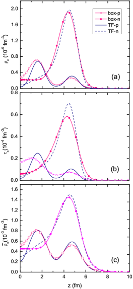
Figure 1: (Color online) Continuum contributions in the energy range from $E_{c}$=40 MeV to $E_{m}$=60 MeV to (a) particle, (b) kinetic, and (c) pairing densities (see Eqs. (14-16)) of ⁷⁰Zn obtained from the TF approximation and discretized box solutions (symbols) of hfb-ax with the SkM* energy density functional and mixed pairing interaction. See text for details.

To examine the quality of the TF approximation for high-energy continuum states, we compared it with the results of box discretization calculations obtained with the HFB solver hfb-ax [Pei08] for ⁷⁰Zn with the SkM^∗ energy density functional (EDF) [Bar82] and mixed pairing interaction. The pairing strength is taken to be $V_{0}=-$234.85 MeV fm^-3 that is adjusted so as to reproduce the neutron pairing gap of ¹²⁰Sn. The calculations have been carried out with the B-spline order of 12; the mesh size 0.6 fm, and the box size 24$\times$24 fm. The nucleus ⁷⁰Zn is predicted to be spherical and has non-vanishing pairing in both protons and neutrons.

Figure 1 displays the continuum contributions to particle, kinetic, and pairing densities due to unbound states from $E_{c}=$40 MeV to $E_{m}=$60 MeV. (In this energy window, the discretized HFB continuum contains no deep-hole resonances.) They were obtained from Eqs. (III.1) and from discretized hfb-ax solutions. It can be seen that the two methods produce very close continuum contributions to the local densities. For the neutrons, the continuum densities are mainly concentrated at the nuclear surface. The proton densities have a more pronounced volume character. We found that this difference is mainly due to different pairing potentials $\Delta(\bm{r})$ and depends weakly on mean-field potentials $V(\bm{r})$. The continuum kinetic and pairing densities have similar shapes to the continuum particle densities. It can be seen, however, that the continuum contributions to pairing densities are larger than to continuum particle densities by two orders of magnitude. This is to be expected: the HFB continuum is strongly affected by the pairing channel dobaczewski96 . Similar conclusions have been obtained in Ref. oba .

It is to be noted that the kinetic and pairing density integrals in Eq. (III.1) are divergent and a finite upper limit for the integration $E_{c}$ must be taken. In practice, the dependence on $E_{c}$ can be avoided by adopting the pairing regularization (21). As discussed in Refs. [Bul02] ; [Yu03] ; [Bor06] , results obtained with regularized pairing are independent on the cutoff energy $E_{c}$ and are very close to the results of a pairing renormalization procedure adopted in this work. Moreover, as also pointed out in Refs. marini ; [Pap99w] , the kinetic energy density $\tau_{c}$ has the same type of divergence as the pairing density $\tilde{\rho}_{c}$, and the sum of kinetic and regularized pairing energies converges.

III.2 The hybrid HFB strategy

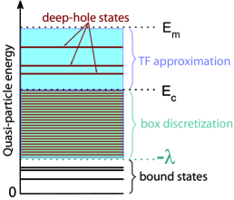
Figure 2: (Color online) Schematic picture of the HFB quasiparticle spectrum. In the energy region $E_{i}\leqslant-\lambda$, quasi-particle states are bound. In the hybrid HFB strategy, the quasi-particle continuum with $E_{i}>-\lambda$ is divided into the low-energy continuum with $-\lambda<E_{i}\leqslant E_{c}$, which is treated by means of the box discretization, and the high-energy continuum with $E_{c}<E_{i}\leqslant E_{m}$ that consists of non-resonant continuum treated by means of the TF approximation and several deep-hole states. See text for details.

We have seen that the Thomas-Fermi approximation to the non-resonant continuum gives results very close to the box discretization approach. This suggests a hybrid HFB strategy to separately treat the deep-hole resonances and the high-energy non-resonant continuum. Figure 2 schematically displays the HFB quasiparticle spectrum. As discussed earlier, the bound HFB solutions exist only in the energy region $E_{i}\leqslant-\lambda$. The quasi-particle continuum with $E_{i}>-\lambda$ consists of non-resonant continuum and quasi-particle resonances. Among the latter ones, the deep-hole states play a distinct role. In the absence of pairing, a deep-hole excitation with energy $E_{i}$ corresponds to an occupied HF state with energy $\varepsilon_{i}=-E_{i}$. If pairing is present, it generates a coupling of this state with unbound particle states with $\varepsilon_{i}\approx-E_{i}$ that gives rise to a quasi-particle resonance with a finite width.

The low-energy continuum with $-\lambda<E_{i}\leqslant E_{c}$ consists of many resonances that have to be computed as precisely as possible. Therefore, to this region we apply the box discretization technique. The high-energy continuum with $E_{c}<E_{i}\leqslant E_{m}$ can be divided into the non-resonant part and several deep-hole states. While the non-resonant continuum can be integrated out by means of the TF approximation, deep-hole states have to be treated separately. Indeed, as discussed in Sec. IV below, deep-hole resonances are sufficiently narrow to be considered as a separate group of states.

To this end, we diagonalize the HF Hamiltonian,

$${}(h-\lambda)v^{\rm HF}_{i}(\bm{r})=\varepsilon_{i}v^{\rm HF}_{i}(\bm{r}),$$ (22)

to obtain wave functions $v^{\rm HF}_{i}(\bm{r})$ and single-particle energies $\varepsilon_{i}$ of deep-hole states. The function $v^{\rm HF}_{i}(\bm{r})$ is a very good approximation to the lower HFB component $v_{i}(\bm{r})$. In the BCS approximation, assuming the state-dependent pairing gap ($\Delta_{i}$ dobaczewski96 ; bender00 ),

$$\Delta_{i}=\int\Delta(\bm{r})[v^{\rm HF}_{i}(\bm{r})]^{2}d{\bm{r}},$$ (23)

the effective BCS occupation factor is:

$$v_{k}^{2}=\displaystyle\frac{1}{2}\left(1-\frac{\varepsilon_{k}}{\sqrt{(\varepsilon_{k})^{2}+\Delta_{k}^{2}}}\right).$$ (24)

Consequently, $v^{\rm HF}_{i}(\bm{r})$ is normalized to the BCS occupation $v_{i}^{2}$. The corresponding quasi-particle energy is related to the single-particle energy through $E_{i}=-\varepsilon_{i}$.

The hybrid HFB strategy is based on combining the box solutions below some low energy cutoff $E_{c}$, the deep-hole solutions, and high-energy TF continuum. In this way, the total particle density (as well as other HFB densities) of the even-even system can be split into three parts:

$$\rho(\bm{r})=\sum\limits_{E_{i}>0}^{E_{c}}2|v_{i}(\bm{r})|^{2}+\sum\limits_{E_{dh}>E_{c}}^{E_{m}}\!\!\!2|v_{dh}^{\rm HF}(\bm{r})|^{2}+\rho_{\rm c}(\bm{r}),$$ (25)

where the continuum particle density $\rho_{\rm c}$ of states between $E_{c}$ and $E_{m}$ is given by Eq. (III.1). In practical applications, the maximum cutoff energy $E_{m}$ is usually taken as 60 MeV$-\lambda$. The continuum contribution to the particle number,

$$N_{c}=\int\rho_{c}(\bm{r})d\bm{r},$$ (26)

is always included to meet the particle number equation.

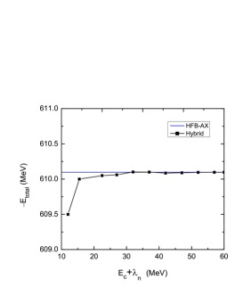
Figure 3: The binding energy of ⁷⁰Zn as a function of the low-energy quasi-particle neutron cutoff $E_{c}$ in the hybrid HFB method. The HFB-AX value corresponds to $E_{c}$=60 MeV+$\lambda$.

We tested this hybrid HFB strategy to calculate the binding energy of ⁷⁰Zn at different cutoff values $E_{c}$. The HF equations (22) are solved using hfb-ax. Generally, the deep-hole single-particle energies $\varepsilon_{i}$ obtained from Eq. (22) are very close to the hole-like solutions of the full HFB diagonalization. In ⁷⁰Zn, for example, the quasi-particle energy of the 1s_1/2 neutron is $E_{i}$=38.071 MeV, while the corresponding HF single-particle energy is $-\varepsilon_{i}$=38.055 MeV.

Figure 3 shows the total binding energy as a function of the neutron cutoff $E_{c}$. It is seen that the total energy is perfectly stable for $E_{c}+\lambda_{n}$$>$30 MeV, and it is equal to the binding energy obtained by means of the full bock discretization ($E_{c}=E_{m}$). At a low value of $E_{c}+\lambda_{n}$$=$15 MeV, the error of the hybrid method is only about 100 keV. At even lower values of cutoff, the TF approximation deteriorates rapidly [Bor06] . Note that the pairing strength in the hybrid HFB should not be renormalized with $E_{c}$. The choice of the cutoff $E_{c}$ is determined by positions of deep-hole levels; this information can be obtained by solving the HF problem. The hybrid strategy can also be modified to work with the pairing regularization procedure [Bor06] . However, as seen in Fig. 3, this technique cannot be used with a very low cutoff $E_{c}$ where resonances are densely populated.

IV Properties of deep-hole resonances of HFB

In this section, we study several approximate methods to calculate widths of HFB resonances. Calculations are performed for ⁷⁰Zn using the SkM^∗ EDF and the mixed pairing interaction.

IV.1 The smoothing and fitting method

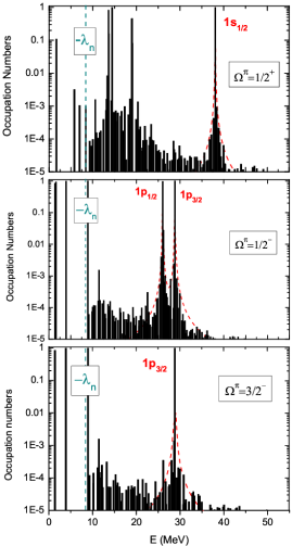
Figure 4: (Color online) Occupation numbers of the discretized neutron quasi-particle continuum states with $\Omega^{\pi}=1/2^{+}$ (top), $\Omega^{\pi}=1/2^{-}$ (middle), and $\Omega^{\pi}=3/2^{-}$ (bottom) calculated for ⁷⁰Zn with hfb-ax. Since ⁷⁰Zn is spherical, angular momenta of discretized resonance states are marked. The corresponding Breit-Wigner envelopes are indicated by dashed lines. Note that the envelopes for $1p_{3/2}$ magnetic substates are identical.

From the box discretization of hfb-ax, one obtains a finite and very dense spectrum of continuum states. The deep-hole states are no longer isolated as in the BCS approximation; they become fragmented due to the pairing coupling with the neighboring particle-like continuum and acquire a decay width. The energy distribution of the occupation numbers

$$v_{i}^{2}=\int|v_{i}(\bm{r})|^{2}\,d\bm{r}$$ (27)

has roughly the Breit-Wigner shape. Figure 4 displays occupation probabilities for the $\Omega^{\pi}$=$1/2^{+}$, $1/2^{-}$, and $3/2^{-}$ discretized neutron quasi-particle states in ⁷⁰Zn as a function of quasi-particle energy $E_{i}$. Note that the angular momentum projection $\Omega$ and parity $\pi$ are good quantum numbers in hfb-ax. It is apparent that the $v_{i}^{2}$ distributions of $1s_{1/2}$, $1p_{3/2}$, and $1p_{1/2}$ deep-hole states have resonance-like structure. For spherical nuclei, degenerate resonances with different values of $|\Omega|$ belonging to the same shell are expected to have the same width, and this is indeed the case for both magnetic substates of $1p_{3/2}$. Breit-Wigner resonance-like structures in occupation probabilities have also been predicted by the recent continuum HFB calculations oba . In the Green function approach Belyaev ; oba , the occupation probability is related to the continuum level density, which corresponds to a Breit-Wigner shape for resonances kruppa99 . In the present work, we propose a straightforward smoothing and fitting method to estimate resonance widths from discrete $v_{i}^{2}$ distributions.

To extract resonance parameters from the discrete distribution of $v_{i}^{2}$, we first smooth it using a Lorentzian shape function $w(x)=1/[2\pi(x^{2}+1/4)]$ arai ; kruppa99 . The occupation numbers $v_{i}^{2}$ of states above the Fermi level are smoothed out by means of folding with $w(E/\Gamma)$,

$$\overline{v^{2}}(E)=\sum_{i}\frac{v_{i}^{2}}{\Gamma}w\Big{(}\frac{E-E_{i}}{\Gamma}\Big{)},$$ (28)

where $\Gamma$ is a smoothing parameter.

The smoothed Breit-Wigner distribution is given by a compact expression arai ; kruppa99 :

$$\begin{array}[]{ll}\overline{v^{2}_{R}}(E)=&\displaystyle\frac{\Gamma_{r}\beta}{2\pi^{2}}\Big{\{}(E-E_{r})^{2}-\frac{(\Gamma^{2}-\Gamma_{r}^{2})}{4}\Big{\}}\vspace{5pt}\\ \vspace{5pt}&\displaystyle\times\Big{\{}\frac{\pi}{2}+\tan^{-1}\big{(}\frac{2E}{\Gamma}\big{)}\Big{\}}\displaystyle+\frac{\Gamma\beta}{2\pi^{2}}\\ \vspace{5pt}&\displaystyle\times\Big{\{}(E-E_{r})^{2}+\frac{(\Gamma^{2}-\Gamma_{r}^{2})}{4}\Big{\}}\\ \vspace{5pt}&\displaystyle\times\Big{\{}\frac{\pi}{2}+\tan^{-1}\big{(}\frac{2E_{r}}{\Gamma}\big{)}\Big{\}}\\ &\displaystyle+\frac{\Gamma_{r}\Gamma}{4\pi^{2}}(E-E_{r})\beta\ln\Big{[}\frac{4E^{2}+\Gamma^{2}}{4E_{r}^{2}+\Gamma_{r}^{2}}\Big{]},\end{array}$$ (29)

where

$$\beta=\big{[}(E-E_{r})^{2}+(\Gamma-\Gamma_{r})^{2}/4\big{]}^{-1}\big{[}(E-E_{r})^{2}+(\Gamma+\Gamma_{r})^{2}/4\big{]}^{-1}.$$ (30)

In the smoothing and fitting method, we fit the smoothed $\overline{v^{2}}(E)$ distribution (28) using a two-term expression:

$${}\overline{v^{2}}(E)=v^{2}\overline{v^{2}_{R}}(E)+v^{2}_{b}(E).$$ (31)

The first term is the smoothed Breit-Wigner resonance shape. The background contribution $v^{2}_{b}(E)$ is assumed to be a slowly changing Fermi-Dirac function $a/(e^{-E/b}+1)$ characterized by parameters $a$ and $b$. In order to deduce the resonance energy $E_{r}$, width $\Gamma_{r}$, and the occupation number $v^{2}$($v^{2}\leqslant 1$), the method of least squares is used.

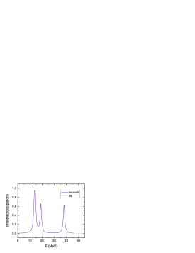
Figure 5: (Color online) Smoothed occupation numbers (28) and the corresponding smoothed Breit-Wigner distribution (29) for the $\Omega^{\pi}=1/2^{+}$ neutron HFB resonances in ⁷⁰Zn.

The results of such a procedure for the $\Omega^{\pi}=1/2^{+}$ neutron HFB resonances in ⁷⁰Zn are illustrated in Fig. 5: the fitted Breit-Wigner resonances agree very well with the smoothed occupation numbers. This demonstrates that the discretized occupation numbers have a Breit-Wigner shape. One has to note, however, that for threshold resonances (such as those close to $E=-\lambda$), the distribution can strongly deviate from Breit-Wigner Grasso .

As it has been pointed out in Ref. kruppa99 , the fitting curve could be dependent on the smoothing parameter $\Gamma$. We checked that such a dependence is not significant as far as the resonance width is concerned if the value of $\Gamma$ around 0.8 MeV is taken. Generally, one should use $\Gamma\gg\Gamma_{r}$. A very small smoothing parameter is not sufficient to smooth out the finite discretization effects. On the other hand, a large smoothing parameter can underestimate the resonance width kruppa99 . Numerical errors can also arise from the fitting procedure if several resonances are overlapping. The discretization can yield a crude representation of occupation distribution if too small a box is used  oba . A high discretization resolution is of particular importance when it comes to narrow resonances. Another advantage of the direct smoothing-fitting method discussed here is that it can be applied to resonances in deformed nuclei.

IV.2 The box stabilization method

The stabilization method hazi is an $\mathcal{L}^{2}$ method, and has been used to obtain precisely the resonance energy $E_{r}$ and widths $\Gamma_{r}$ in atomic mandelshtam94 ; ryaboy ; Salzgeber and nuclear zhang1 ; zhou physics. Based on the box solutions, the HFB resonances are expected to be localized solutions with energies weakly affected by changes of the box size. The stabilization method allows to obtain the resonance parameters from the box-size dependence of quasi-particle eigenvalues.

To this end, one introduces the continuum level density $\Delta(E)$,

$$g(E)={\rm Tr}[\delta(E-H)-\delta(E-H_{0})],$$ (32)

where $H_{0}$ is the non-interacting Hamiltonian of the system. The continuum level density is related to the phase shift by

$$\delta(E)=\pi\int_{0}^{E}g(E^{\prime})\,dE^{\prime}.$$ (33)

In a modified stabilization method, one can obtain the phase shift using the box-discretized continuum mandelshtam94 . Firstly, we compute quasi-particle energies $E_{j}(L)$ with different box size ${L}$ using the spherical HFB solver hfbrad HFBRAD .

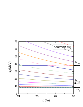
Figure 6: (Color online) The neutron discretized quasi-particle $\ell$=0 spectrum of ⁷⁰Zn as a function of the box size $L$. Calculations have been carried out with the spherical HFB solver hfbrad HFBRAD . Unlike the non-resonant box continuum, resonances are practically $L$-independent.

Figure 6 shows that the discretized quasi-particle energies generally smoothly decrease as the box size increases. Around the resonances, however, the energies are fairly constant. Starting from a sufficiently large box $L_{0}$, calculations are done on a grid with the spacing $\delta L$:

$${}L=L_{0}+\Delta L,~{}~{}~{}\Delta L=(M-1)\delta L.$$ (34)

In this way, eigenvalues $E_{j}$ are stored in arrays $E_{j}(L)$. By using the Akima interpolation akima , we obtain the values of $L_{j}(E)$ corresponding to a box size with which the $j^{\rm th}$ eigenvalue equals to $E$.

In the next step, the phase shift is obtained from mandelshtam94 :

$${}\delta(E)=\pi N(E)+\frac{\pi}{\Delta L}\sum_{j}(L_{0}+\Delta L-L_{j}(E)),$$ (35)

where $N(E)$ is the number of eigenvalues for which $E_{j}(L_{0})<E$. To obtain the resonance energy $E_{r}$ and the width $\Gamma_{r}$, we fit the phase shift $\delta(E)$ by using the expression:

$$\tilde{\delta}(E)=\arctan\left(\frac{2(E-E_{r})}{\Gamma_{r}}\right)+\tilde{\delta}_{b}(E),$$ (36)

where $\tilde{\delta}_{b}(E)$ represents the smoothly changing background contribution parametrized as:

$${}\tilde{\delta}_{b}(E)=a+b(E-E_{r}).$$ (37)

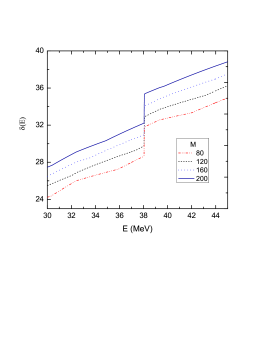
Figure 7: The phase shifts $\delta(E)$ of the neutron 1s_1/2 state of ⁷⁰Zn obtained with the stabilization method with different iteration steps (34). Here, $\delta L$=0.06 fm and $L_{0}$=24 fm.

Figure 7 shows the phase shifts of the neutron 1s_1/2 resonance obtained with different step numbers $M$. It can be seen that the background becomes more smooth as the step numbers increase. Generally, a large $\Delta L$ is necessary to smooth out the background, so as to reduce the fitting errors in $a$ and $b$ in Eq. (37). In our calculation, we also find that for very narrow resonances, a small value of $\delta L$ is important for the interpolation precision. In principle, as

$$\delta L\rightarrow 0~{}~{}~{}{\rm and}~{}~{}~{}\Delta L\rightarrow\infty,$$ (38)

one can get very accurate resonance parameters. In practice, however, calculations with a large box and small step sizes are very expensive even with a fast hfbrad solver. The eigenvalue spectrum of hfbrad is sparse, resulting in statistical errors in the calculations of phase shift. For low-energy HFB resonances, this situation is even worse since these eigenvalues change very slowly as the box size increases, as shown in Fig. 6. In this case, the calculated background is not sufficiently smooth. Currently, the stabilization method is limited to spherical boxes as in hfbrad. The extension of the stabilization method to deformed cases will be the subject of future work.

IV.3 The perturbative expression

Assuming that the pairing coupling can be treated perturbatively, the width of a deep-hole HFB resonance can be given by the Fermi Golden rule  bulgac80 ; Belyaev ; dobaczewski96 :

$${}\Gamma=2\pi|\langle u_{0E}|\Delta|v^{\rm HF}|\rangle|^{2},$$ (39)

where $\Delta$ is the pairing potential; $v^{\rm HF}$ is the bound wave function of the HF potential corresponding to the single-particle energy $-E+\lambda$, and $u_{0E}$ is the scattering solution of the HF equation with energy $E+\lambda$.

At a large distance, the scattering wave function $u_{0E}$ has the usual asymptotic form:

$$u_{0E}={1\over r}\sqrt{\frac{2m}{\hbar^{2}\pi k}}\left(\cos\delta_{l}F_{l}(\eta,kr)+\sin\delta_{l}G_{l}(\eta,kr)\right),$$ (40)

where $F_{l}$ and $G_{l}$ are the regular and irregular Coulomb functions, respectively; $\delta_{l}$ is the phase shift; and $k=\sqrt{2m(E+\lambda)/\hbar^{2}}$. The scattering wave function is found with the help of Ref. papp . In the calculation of scattering wave functions, $\hbar^{2}/2m$ is taken as a constant 20.734 MeV, to avoid problems related to the density-dependent effective mass.

Table 1: Energies (in MeV) and widths (in keV) of deep-hole HFB resonances in ⁷⁰Zn calculated with the box stabilization method (box), smoothing-fitting method (smf), and perturbative expression (per). See text for more details.

	Neutron				Proton
states	E	$\Gamma_{\rm box}$	$\Gamma_{\rm smf}$	$\Gamma_{\rm per}$	E	$\Gamma_{\rm box}$	$\Gamma_{\rm smf}$	$\Gamma_{\rm per}$
$1s_{1/2}$	38.075	1.23	0.80	0.98	35.147	0.64	0.54	0.40
$1p_{3/2}$	28.801	3.42	4.1	0.04	25.424	3.22	2.04	2.27
$1p_{1/2}$	26.043	6.01	7.0	0.19	22.851	2.04	1.57	1.26
$1d_{5/2}$	18.987	13.1	10.6	22.7	15.320	-	0.12	0.09

Table 1 displays the widths of high-energy deep-hole states in ⁷⁰Zn calculated with the smoothing-fitting method, box stabilization method, and perturbative expression. It is seen that the widths obtained with the smoothing-fitting method and box stabilization method are always fairly close. For protons, all three methods yield similar results. However, the perturbative expression predicts widths that are too small for the 1p_3/2 and 1p_1/2 neutron states. The difference is due to a surface-peaked neutron pairing potential that is very different from that of protons (see Fig.1). Indeed, for surface-peaked pairing, the overlap between $u_{0E}$ (which exhibits rapid spatial oscillations), $v^{\rm HF}$, and $\Delta(r)$ is too sensitive to small changes in $u_{0E}$. For more discussion on limitations of the perturbative expression (39), see also the schematic model analysis in Ref. Belyaev .

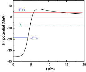
Figure 8: (Color online) A special kind of deep-hole HFB proton resonance, in which the upper component of the HFB wave function is quasi bound, due to the confining effect of the Coulomb-plus-centrifugal barrier.

Compared to other deep-hole resonances in Table 1, the width of the proton 1d_5/2 state is very small. This is because the upper component wave function of this $\ell=2$ state is quasi bound, due to the confining effect of the Coulomb-plus-centrifugal barrier (see Fig. 8). For such narrow resonances, the stabilization method cannot easily be applied.

V applications to weakly bound nuclei

The effects of continuum are expected to increase when moving towards the neutron drip line [Dob97a] . Especially for very weakly bound nuclei exhibiting halo structures, there exists a strong interplay between pairing and continuum [Ben00] ; [Yam05] ; [Hag11] . Here, we investigate the role of continuum contributions in the neutron-rich Ni isotopes. These nuclei have been studied by the Gamow HFB (GHFB) method and the exact quasi-particle resonance widths of ⁹⁰Ni are available Michel . The GHFB work provides an excellent benchmark for our approximate resonance widths.

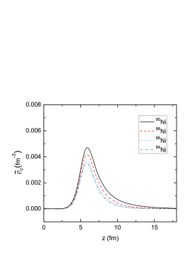
Figure 9: (Color online) The continuum contributions to the neutron pairing densities of neutron-rich ^84,86,88,90Ni isotopes, calculated with Eq. (III.1) with $E_{c}$=30 MeV and $E_{m}$=60 MeV and mixed pairing interaction. See text for details.

As in Ref. Michel , the calculations have been carried out with the SLy4 EDF sly4 and the surface pairing interaction [Dob02c] , with the strength $V_{0}$=$-$519.9 MeV fm^-3. In Fig.9, we show the high-energy continuum contributions to the neutron pairing densities in ^84,86,88,90Ni, obtained using the TF approximation (III.1). It can be seen that the continuum pairing density acts in the surface region, and increases as nuclei become less bound. This is consistent with the earlier findings dobaczewski96 that continuum becomes important for nuclei close to the drip line.

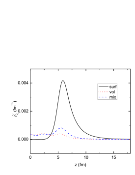
Figure 10: (Color online) Similar to Fig. 9 but with the volume, surface, and mixed pairing interaction in ⁸⁸Ni.

Figure 10 illustrates the interaction dependence of the pairing-continuum effect. Namely, it displays the neutron continuum pairing densities for ⁸⁸Ni with the volume pairing ($V_{0}$=$-$185.026 MeV fm^-3), surface pairing as in Fig.9, and mixed pairing ($V_{0}$=$-$284.36 MeV fm^-3). (The pairing strengths $V_{0}$ have all been adjusted to reproduce the neutron pairing gap of ¹²⁰Sn.) It is seen that the high-energy continuum contribution to pairing density strongly depends on character of pairing interaction Belyaev ; dobaczewski96 . In particular, in the case of surface pairing, the continuum contribution is remarkably larger than for other two pairing functionals, indicating its very different behavior in weakly bound nuclei [Dob01a] . Actually, as it has been discussed [Pei08] the surface pairing is essential for the existence of bound ⁹⁰Ni.

Table 2: Energies (in MeV) and widths (in keV) of HFB neutron resonances in ⁹⁰Ni, calculated using the box stabilization (box) and smoothing-fitting (smf) methods. They are compared to the GHFB solutions of Ref. Michel .

states	$E_{r}$	$\Gamma_{\rm box}$	$\Gamma_{\rm smf}$	$\Gamma_{\rm GHFB}$
$1s_{1/2}$	51.419	-	1.1e-3	1.09e-3
$1p_{3/2}$	40.588	30.84	20.17	27.28
$1p_{1/2}$	38.770	32.26	34.67	27.14
$1d_{5/2}$	29.039	1.31	1.37	0.78
$1d_{3/2}$	25.017	25.44	23.08	22.57
$2s_{1/2}$	24.319	50.36	40.87	46.00
$1f_{7/2}$	17.554	401.79	413.04	397.37
$2p_{3/2}$	12.538	499.98	471.22	490.56
$1f_{5/2}$	10.981	672.44	651.12	645.64
$2p_{1/2}$	10.816	440.76	376.19	404.30
$1g_{9/2}$	6.519	1.56	0.52	0.81
$2d_{5/2}$	3.270	221.08	105.17	194.18
$2d_{3/2}$	2.310	611.50	643.88	560.61
$1g_{7/2}$	3.348	69.09	75.13	63.61
$1h_{11/2}$	5.527	162.46	173.66	131.78

Table 2 displays the widths of neutron resonances in ⁹⁰Ni calculated using different techniques. In the calculations with the box stabilization method, we used $L_{0}$=22 fm, $M$=400, and $\delta L$=0.06 fm, see Eq.  (34). Figure 11 illustrates the quality of calculations for the neutron 1p_3/2 resonance. It is seen that the fitted phase shift agrees well with that obtained from the stabilization method. Systematically, the box stabilization method predicts slightly larger widths as compared to GHFB. This is consistent with findings of Ref. ryaboy where the stabilization method generally overestimates the widths by 10$\%$. In particular, it is shown that the widths of very narrow resonances are largely overestimated. The width of the 1s_1/2 state is so narrow that it is beyond the applicability of the stabilization method. The very narrow 1g_9/2 state belongs to the class of special HFB resonances of Fig.8. Among the resonances, the 1g_7/2 and 1h_11/2 states are also single-particle resonances in the Hartree-Fock theory Michel . Other than that, Table 2 demonstrates that the stabilization method works well for all the HFB resonances except for extremely narrow ones.

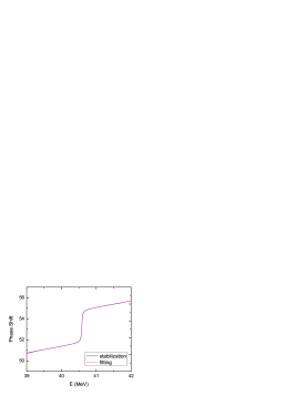
Figure 11: (Color online) The phase shift of the neutron 1p_3/2 resonance in ⁹⁰Ni using Eqs. (37) and (35).

Within the smoothing-fitting method, the quasi-particle energy spectrum is obtained by hfb-ax by taking a large box of 38$\times$38 fm. The widths given by the smoothing-fitting method agree with the exact numbers within a factor of two. We have found that the fitting precision is compromised when several resonances overlap. For the low-energy resonances, the total occupation numbers $v^{2}$ in Eq.(31) are very small and can induce additional fitting errors. Besides, as we have discussed earlier, it is not proper to fit the occupation probabilities of low-energy resonances near the Fermi energy using a Breit-Wigner shape. In spite of all those reservations, the precision of the smoothing-fitting method is quite satisfactory.

For neutron HFB resonance widths in Ni isotopes, our calculations predict that generally the widths would slowly increase as the drip line is approached. For example, the widths of the neutron 1p_3/2 state in ⁸⁶Ni, ⁸⁸Ni, and ⁹⁰Ni calculated by the stabilization method are, respectively, 25.97 keV, 28.25 keV, and 30.84 keV. This is consistent with Fig. 9: the widths grow with the increased pairing-continuum coupling.

VI Conclusions

In this work, we performed a comprehensive study of quasi-particle continuum within the HFB theory. The purpose of this investigation is twofold. Firstly, we tested a truncation scheme based on the Thomas-Fermi approximation to limit the continuum space in realistic calculations carried out in huge configuration spaces (or large spatial boxes) that yield huge amounts of discretized unbound states. Secondly, we studied properties of HFB resonances, including deep-hole states. We compare several methods to estimate resonance width and discuss their strengths and weaknesses.

The TF approximation to the high-energy continuum states in the hybrid HFB variant, in which deep-hole states and non-resonant continuum are separately treated, has been found very effective for it fully reproduces results obtained with the full box discretization. The high-energy non-resonant continuum has been found to have a similar spatial behavior for particle, kinetic, and pairing densities. This distribution is mainly determined by the pairing potential. The continuum contribution to the pairing density is substantial for weakly bound nuclei and it has appreciable spatial extension. The hybrid method will be useful in reducing the computational cost of 3D coordinate-space HFB calculations.

The HFB quasi-particle resonance is unique to the HFB theory and is a fascinating topic in its own right. We examined three approximate methods to study the resonance widths based on HFB box solutions. In the smoothing-fitting method, resonance parameters are obtained by fitting the smoothed occupation numbers obtained from discretized solutions. The box stabilization method is based on the fact that quasi-particle energies of continuum states change with the box size. By comparing with the exact Gamow HFB results obtained by imposing outgoing boundary conditions Michel , we have demonstrated that the stabilization method works fairly well for all HFB resonances, except for the very narrow ones. The smoothing-fitting method is also very effective and can easily be extended to deformed cases. The perturbative Fermi golden rule is found to be unreliable for calculating widths of neutron resonances. The only exceptions are narrow metastable deep-hole states such as high-$\ell$ states and low-lying proton resonances.

Illustrative examples have been provided for the drip-line Ni isotopes. We found that continuum densities strongly depend on the density dependence of pairing interaction. In particular, surface pairing produces very large continuum pairing densities. The obtained neutron widths of ⁹⁰Ni are generally larger than that of stable nuclei. The presence of broad quasi-particle resonances in weakly bound nuclei suggests that quasi-particle continuum plays an important role in the description of excited states. In addition, we expect that the determination of neutron resonance widths can be useful to estimate neutron emission half-lives of excited states above the neutron emission threshold.

In summary, we have demonstrated that one can implement powerful approximations to incorporate the vast quasi-particle continuum space without explicitly imposing scattering or outgoing boundary conditions. We expect our work can also be useful in the context of continuum-QRPA applications. The approximate techniques used in this study have demonstrated the precision of the box discretization in representing the continuum and deep-hole resonances, especially important for nuclei near drip lines where continuum effects are large.

- (1) J. Dobaczewski, N. Michel, W. Nazarewicz, M. Płoszajczak, and J. Rotureau, Prog. Part. Nucl. Phys. 59, 432 (2007).
- (2) M. Bender, P.-H. Heenen, and P.-G. Reinhard, Rev. Mod. Phys. 75, 121 (2003).
- (3) S.G. Rohoziński, J. Dobaczewski, and W. Nazarewicz, Phys. Rev. C 81, 014313 (2010).
- (4) A. Bulgac, Preprint FT-194-1980, Central Institute of Physics, Bucharest, 1980; nucl-th/9907088.
- (5) J. Dobaczewski, H. Flocard and J. Treiner, Nucl. Phys. A 422, 103 (1984).
- (6) S.T. Belyaev, A.V. Smirnov, S.V. Tolokonnikov, and S.A. Fayans, Sov. J. Nucl. Phys. 45, 783 (1987).
- (7) J. Dobaczewski, W. Nazarewicz, T.R. Werner, J.F. Berger, C.R. Chinn, and J. Dechargé, Phys. Rev. C 53, 2809 (1996).
- (8) N. Michel, K. Matsuyanagi, and M. Stoitsov, Phys. Rev. C 78, 044319 (2008).
- (9) R. Id Betan, N. Sandulescu, and T. Vertse, Nucl. Phys. A 771, 93 (2006).
- (10) R. Id Betan, G.G. Dussel, and R.J. Liotta, Phys. Rev. C 78, 044325 (2008).
- (11) S.A. Fayans, S.V. Tolokonnikov, E.L. Trykov, and D. Zawischa, JETP Letters 68, 276 (1998).
- (12) J. Dobaczewski, W. Nazarewicz, and P.-G. Reinhard, Nucl. Phys. A 693, 361 (2001).
- (13) M. Grasso, N. Sandulescu, Nguyen Van Giai, and R.J. Liotta, Phys. Rev. C 64, 064321 (2001).
- (14) M. Grasso, N. Van Giai, and N. Sandulescu, Phys. Lett. B 535, 103 (2002).
- (15) A. Bulgac and Y. Yu, Phys. Rev. Lett. 88, 042504 (2002).
- (16) Y. Yu and A. Bulgac, Phys. Rev. Lett. 90, 222501 (2003).
- (17) P.J. Borycki, J. Dobaczewski, W. Nazarewicz, and M.V. Stoitsov, Phys. Rev. C 73, 044319 (2006).
- (18) E. Terán, V.E. Oberacker, and A.S. Umar, Phys. Rev. C 67, 064314 (2003).
- (19) N. Schunck and J.L. Egido, Phys. Rev. C 77, 011301 (2008).
- (20) H. Oba and M. Matsuo, Phys. Rev. C 80, 024301 (2009).
- (21) Y. Zhang, M. Matsuo, J. Meng, Phys. Rev. C 83, 054301 (2011).
- (22) V. Rodin, A. Faessler, Prog. Part. Nucl. Phys. 57, 226 (2006).
- (23) K. Hagino, Nguyen Van Giai, and H. Sagawa, Nucl. Phys. A 731, 264 (2004).
- (24) J. Terasaki, J. Engel, M. Bender, J. Dobaczewski, W. Nazarewicz, and M. Stoitsov, Phys. Rev. C 71, 034310 (2005).
- (25) J. Terasaki and J. Engel, Phys. Rev. C 74, 044301 (2006).
- (26) K. Mizuyama, M. Matsuo, and Y. Serizawa, Phys. Rev. C 79, 024313 (2009).
- (27) N. Michel, W. Nazarewicz, M. Płoszajczak, and K. Bennaceur, Phys. Rev. Lett. 89, 042502 (2002).
- (28) N. Michel, W. Nazarewicz, M. Płoszajczak, and T. Vertse, J. Phys. G 36, 013101 (2009).
- (29) M. Stoitsov, N. Michel, and K. Matsuyanagi, Phys. Rev. C 77, 054301 (2008).
- (30) K. Bennaceur and J. Dobaczewski, Compt. Phys. Comm. 168, 96 (2005).
- (31) M. Yamagami, Phys. Rev. C 72, 064308 (2005) and arXiv:nucl-th/0504059v1.
- (32) J. C. Pei, M. V. Stoitsov, G. I. Fann, W. Nazarewicz, N. Schunck, and F. R. Xu, Phys. Rev. C78, 064306 (2008).
- (33) V.E. Oberacker, A. S. Umar, E. Terán, and A. Blazkiewicz, Phys. Rev. C 68, 064302 (2003).
- (34) J.C. Pei, W. Nazarewicz, and M. Stoitsov, Eur. Phys. J. A 42, 595 (2009).
- (35) G.I. Fann, J. Pei, R.J. Harrison, J. Jia, J. Hill, M. Ou, W. Nazarewicz, W.A. Shelton, and N. Schunck, J. Phys. Conf. Ser. 180, 012080 (2009).
- (36) J. Reidl, A. Csordás, R. Graham, and P. Szépfalusy, Phys. Rev. A 59, 3816 (1999).
- (37) X.J. Liu, H. Hu, and P.D. Drummond, Phys. Rev. A 76, 043605 (2007); Phys. Rev. A 78, 023601 (2008).
- (38) A.U. Hazi and H.S. Taylor, Phys. Rev. A 1, 1109 (1970).
- (39) V. Ryaboy, N. Moiseyev, V.A. Mandelshtam, and H.S. Taylor, J. Chem. Phys. 101, 5677 (1994).
- (40) V.A. Mandelshtam, H.S. Taylor, V. Ryaboy, and N. Moiseyev, Phys. Rev. A 50, 2764 (1994).
- (41) A.T. Kruppa and K. Arai, Phys. Rev. A 59, 3556 (1999).
- (42) N. Van Giai and E. Khan, in Extended Density Functionals in Nuclear Structure Physics, ed. by G.A. Lalazissis, P. Ring, and D. Vretenar (Springer Verlag, 2004).
- (43) J. Dobaczewski, W. Nazarewicz, and M.V. Stoitsov, Eur. Phys. J. A 15, 21 (2002).
- (44) J. Bartel, P. Quentin, M. Brack, C. Guet, and H.B. Håkansson, Nucl. Phys. A 386, 79 (1982).
- (45) M. Marini, F. Pistolesi, and G.C. Strinati, Eur. Phys. J. B 1, 151 (1998).
- (46) T. Papenbrock and G.F. Bertsch, Phys. Rev. C 59, 2052 (1999).
- (47) M. Bender, K. Rutz, P.-G. Reinhard, and J.A. Maruhn, Eur. Phys. J A 8, 59 (2000).
- (48) K. Arai and A.T. Kruppa, Phys. Rev. C 60, 064315 (1999).
- (49) R.F. Salzgeber, U. Manthe, Th. Weiss, and Ch. Schlier, Chem. Phys. Lett. 249, 237 (1996).
- (50) L. Zhang, S.G. Zhou, J. Meng, and E.G. Zhao, Phys. Rev. C 77, 014312 (2008).
- (51) S.G. Zhou, J. Meng, P. Ring, and E.G. Zhao, Phys. Rev. C 82, 011301(R) (2010).
- (52) The IMSL numerical library, see http://www.vni.com/products/imsl/.
- (53) Z. Papp, Comp. Phys. Commun. 70, 435(1992).
- (54) J. Dobaczewski and W. Nazarewicz, Phil. Trans. R. Soc. Lond. A 356, 2007 (1998).
- (55) K. Bennaceur, J. Dobaczewski, and M. Płoszajczak, Phys. Lett. B496, 154 (2000).
- (56) M. Yamagami, Eur. Phys. A 25, s01, 569 (2005).
- (57) K. Hagino and H. Sagawa, Phys. Rev. C (2011); arXiv:1105.5469v1.
- (58) E. Chabanat, P. Bonche, P. Haensel, J. Meyer, and R. Schaeffer, Nucl. Phys. A 635, 231 (1998).