Multiresolution analysis for Markov Interval Maps

Abstract.

We set up a multiresolution analysis on fractal sets derived from limit sets of Markov Interval Maps. For this we consider the $\mathbb{Z}$-convolution of a non-atomic measure supported on the limit set of such systems and give a thorough investigation of the space of square integrable functions with respect to this measure. We define an abstract multiresolution analysis, prove the existence of mother wavelets, and then apply these abstract results to Markov Interval Maps. Even though, in our setting the corresponding scaling operators are in general not unitary we are able to give a complete description of the multiresolution analysis in terms of multiwavelets.

1. Introduction and main results

The main aim of this paper is to construct a wavelet basis on limit sets of Markov Interval Maps (MIM) in the unit interval translated by $\mathbb{Z}$. In this way we extend the results in [DJ06, BK10], where wavelet bases with respect to singular measures were provided. For this we first prove that a MIM gives rise to a multiresolution analysis (MRA) and study the particular case where the underlying measure is Markovian. This MRA is then reformulated in an abstract way allowing us to prove the existence of a wavelet basis in this abstract setting.

In the case of a fractal given by an iterated function system (IFS) on $[0,1]$ there are several approaches to construct a wavelet basis on the $L^{2}$-space with respect to a suitable singular measure which is supported on a so-called enlarged fractal. The enlarged fractal is derived from the original fractal by first mapping scaled copies of it to each gap interval and then by taking the union of translats by $\mathbb{Z}$ defining a dense set in $\mathbb{R}$. In [DJ06] the authors construct a wavelets basis for fractals on self-similar Cantor sets, i.e. sets that are given by affine IFS with the same scaling factor $1/N$, $N\geq 2$, for all $p\leq N$ branches. They consider the $L^{2}$-space with respect to $\mu$, the $\delta$-dimensional Hausdorff measure restricted to the enlarged fractal, where $\delta$ denotes the dimension of the Cantor set. In this situation the analysis depends on the two unitary operators $U$ and $T$, where $U$ denotes the scaling operator given by $Uf:=\sqrt{p}f\left(N\cdot\right)$ and $T$ denotes the translation operator given by $Tf:=f(\cdot-1)$ for $f\in L^{2}(\mu)$. Furthermore, a natural choice for a father wavelet $\varphi$ is the characteristic function on the original fractal. The authors show that for a family of closed subspaces $\left(V_{j}\right)_{j\in\mathbb{Z}}$ of $L^{2}(\mu)$ the following six conditions are satisfied.

• $\dots\subset V_{-2}\subset V_{-1}\subset V_{0}\subset V_{1}\subset V_{2}\subset\cdots$,

• $\text{cl}\bigcup_{j\in\mathbb{Z}}V_{j}=L^{2}(\mu)$,

• $\bigcap_{j\in\mathbb{Z}}V_{j}=\{0\}$,

• $V_{j+1}=UV_{j}$, $j\in\mathbb{Z}$,

• $\left\{T^{n}\varphi:\;n\in\mathbb{Z}\right\}$ is an orthonormal basis in $V_{0}$,

• $U^{-1}TU=T^{N}$.

These observations allow the authors to construct a wavelets basis for $L^{2}(\mu)$ explicitly in terms of certain filter functions.

In [BK10] we generalize this approach by allowing conformal IFS satisfying the open set condition on $[0,1]$. We choose the measure of maximal entropy supported on the fractal and this measure is extended to a measure $\mu$ supported on the enlarged fractal in $\mathbb{R}$. Then similarly as in [DJ06] we construct the wavelet basis via MRA in terms of the unitary scaling operator $U$ and the unitary translation operator $T$. Again via filter functions the mother wavelets $\psi_{i}$, $i\in\left\{1,\dots,N-1\right\}$ are defined such that $\left\{U^{n}T^{k}\psi_{i}:n,k\in\mathbb{Z},i\in\{1,\dots,N-1\}\right\}$ provides an orthonormal basis of $L^{2}(\mu)$.

Here, our aim is to extend the construction of wavelet bases with respect to fractal measures to the construction of wavelet bases on the by $\mathbb{Z}$ translated limit set of a Markov Interval Map (MIM). A Markov Interval Map consists of a family $\left(B_{i}\right)_{i=0}^{N-1}$ of closed subintervals in $[0,1]$ with disjoint interior, and a function $F:\bigcup_{i\in\underline{N}}B_{i}\rightarrow[0,1]$, such that $F|{}_{B_{i}}$ is expanding and $C^{1}$, $i\in\underline{N}:=\left\{0,\ldots,N-1\right\}$ and such that $F\left(B_{i}\right)\cap B_{j}\not=\varnothing$ implies $B_{j}\subset F\left(B_{i}\right)$. Its (fractal) limit set is given by $X:=\bigcap_{n=0}^{\infty}F^{-n}I$, where $I:=\bigcup_{i\in\underline{N}}B_{i}$. By considering its inverse branches $\tau_{i}:=\left(F|_{B_{i}}\right)^{-1}$, $i\in\underline{N}$, we obtain a Graph Directed Markov System (see [MU03]) with incidence matrix $A=\left(A_{ij}\right)_{i,j\in\underline{N}}$, where $A_{ij}=1$ if $F\left(B_{i}\right)\supset B_{j}$ and $0$ otherwise. For the precise definition see Definition 2.1 and for an explicit example of an MIM see Example 1.2 where we consider the $\beta$-transformation. The limit set $X$ is – up to a countable set where it is finite-to-one – homeomorphic to the topological Markov chain $\Sigma_{A}:=\{\omega=(\omega_{0},\omega_{1},\dots)\in\underline{N}^{\mathbb{N}}:\,A_{\omega_{i}\omega_{i+1}}=1\,\forall i\geq 0\}$. For the definition of the canonical coding map $\pi$ from $\Sigma_{A}$ to $X$ see (2.1).

Given a Markov measure $\widetilde{\nu}$ on the shift space $\Sigma_{A}$ with a probability vector $\left(p_{i}\right)_{i\in\underline{N}}$ and stochastic matrix $\left(\pi_{ij}\right)_{i,j\in\underline{N}}$, we consider the probability measure $\nu:=\widetilde{\nu}\circ\pi^{-1}$, to which we also refer as $\nu$ a Markov measure. The $\mathbb{Z}$-convolution (by translations) of $\nu$ is given by

$$\nu_{\mathbb{Z}}:=\sum_{k\in\mathbb{Z}}\nu(\cdot-k).$$

Similar to the construction in [BK10] we introduce the scaling operator

(1.1) $$Uf(x):=\sum_{k\in\mathbb{Z}}\sum_{j\in\underline{N}}\sum_{i\in\underline{N}}\sqrt{\frac{p_{i}}{p_{j}\pi_{ji}}}\cdot\mathbbm{1}_{[ji]}(x-k)\cdot f(\tau_{j}^{-1}(x-k)+j+Nk)$$

and the translation operator

(1.2) $$Tf(x):=f(x-1)$$

for $f\in L^{2}(\nu_{\mathbb{Z}})$ and $x\in\mathbb{R}$, where $[ji]\subset\mathbb{R}$, $i,j\in\underline{N}$, denotes a cylinder set (see Section 2). It is important to note that in contrast to the construction of the scaling operator for IFS the operator $U$ is in general not unitary. Nevertheless, we have the following properties.

Proposition 1.1.

Let $\left(\varphi_{i}\right)_{i\in\underline{N}}$ denote a family of father wavelets given by $\varphi_{i}:=\sqrt{\nu([i])}^{-1}\mathbbm{1}_{[i]}$, $i\in\underline{N}$. The translation operator $T$ and the scaling operator $U$ satisfy the following properties.

1. $TU=UT^{N}$,

2. $\varphi_{i}=U\sum_{j\in\underline{N}}\sqrt{\pi_{ij}}T^{i}\varphi_{j}$, $i\in\underline{N}$,

3. $\langle T^{k}\varphi_{i}|T^{l}\varphi_{j}\rangle=\delta_{(k,i),(l,j)}$, $k,l\in\mathbb{Z}$, $i,j\in\underline{N}$,

4. $UU^{*}=\operatorname{id}$,

5. $U^{*}U=\operatorname{id}$ if and only if $A_{ij}=1$ for all $i,j\in\underline{N}.$

For an explicit formula of $U^{*}$ see (4.2). As an example for this setting we consider the $\beta$-transformation.

Example 1.2 ($\beta$-Transformation).

Let $\beta:=\frac{1+\sqrt{5}}{2}$ denote the golden mean. Then the $\beta$-transformation is given by $F:\left[0,1\right]\to\left[0,1\right]$, $x\mapsto\beta x\mod 1$ (see Figure 1.1 for the graph of $F$). This map can be considered as a MIM as follows. In this case we have $X:=[0,1]$ and the inverse branches are $\tau_{0}(x):=\frac{x}{\beta}$, $x\in[0,1]$, and $\tau_{1}(x):=\frac{x+1}{\beta}$, $x\in[0,\beta-1]$. We may choose the two intervals $B_{0}:=[0,\beta-1]$ and $B_{1}:=[\beta-1,1]$ and the corresponding transition matrix is then given by $A:=\left(\begin{array}[]{cc}1&1\\ 1&0\end{array}\right)$.

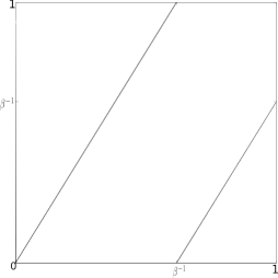
Figure 1.1. The graph of the $\beta$-transform.

From [Rén57, Par60] we know that there exists an invariant measure $\nu$ absolutely continuous to the Lebesgue measure restricted to $[0,1]$ with density $h$ given by

$$h(x):=\begin{cases}\frac{5+3\sqrt{5}}{10}&\text{for}\,\,0\leq x<\frac{\sqrt{5}-1}{2},\\ \frac{5+\sqrt{5}}{10}&\text{for}\,\,\frac{\sqrt{5}-1}{2}\leq x<1.\end{cases}$$

The measure $\nu$ can be represented on $\Sigma_{A}$ by a stationary Markov measure with the stochastic matrix

$$\Pi:=\left(\begin{array}[]{cc}\beta-1&2-\beta\\ 1&0\end{array}\right)$$

and probability vector $p:=\left(\frac{\beta}{\sqrt{5}},\frac{\beta-1}{\sqrt{5}}\right)$. The scaling operator $U$ acting on $L^{2}\left(\nu_{\mathbb{Z}}\right)$ is then given for $x\in\mathbb{R}$ by

$$Uf(x)= \sum_{k\in\mathbb{Z}}\Big{(}\sqrt{\beta}\mathbbm{1}_{[0,\beta^{-2})}(x-k)+\mathbbm{1}_{[\beta^{-2},\beta^{-1})}(x-k)$$

$$\,\,\,\,\,\,\,\,+\beta\cdot\mathbbm{1}_{[\beta^{-1},1)}(x-k)\Big{)}\cdot f\left(\beta(x-k)+2k\right).$$

For the father wavelets we may choose $\varphi_{0}=\left(\sqrt{5}/\beta\right)^{1/2}\mathbbm{1}_{[0,\beta-1)}$ and $\varphi_{1}=\left(\sqrt{5}\beta\right)^{1/2}\mathbbm{1}_{[\beta-1,1)}$. We illustrate the action of $U$ in Figure 1.2 where $U$ is applied to the identity map $\operatorname{id}_{\left[0,1\right]}:x\mapsto x$, restricted to $\left[0,1\right]$, that is for $x\in[0,1]$ we have

$$U\left(\operatorname{id}_{\left[0,1\right]}\right)x=\left(\sqrt{\beta}\mathbbm{1}_{[0,\beta^{-2})}(x)+\mathbbm{1}_{[\beta^{-2},\beta^{-1})}(x)+\beta\cdot\mathbbm{1}_{[\beta^{-1},1)}(x)\right)\beta x.$$

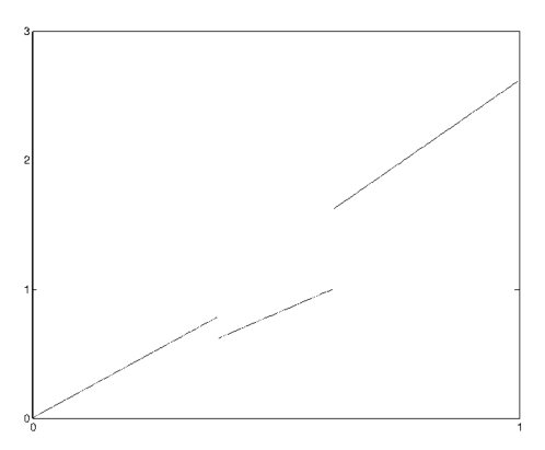
Figure 1.2. The graph of $U\left(\operatorname{id}_{[0,1]}\right)$.

We further generalize our construction by considering non-atomic probability measures $\nu$ on $X$ which we do not assume to be Markovian. In this case it is natural to consider more than just one scaling operator $U$. More precisely, we consider a family of scaling operators $\left(U^{(n)}\right)_{n\in\mathbb{Z}}$ which allow us to construct an orthonormal wavelet basis. For this we define $U^{(0)}:=\operatorname{id}$ and for $f\in L^{2}(\nu_{\mathbb{Z}})$ and $n\in\mathbb{N}$ we let

(1.3) $$\begin{array}[]{ll}U^{(n)}f(x)&:={\displaystyle\sum_{k\in\mathbb{Z}}\sum_{\omega\in\Sigma_{A}^{n}}\sum_{j\in\underline{N}}\sqrt{\frac{\nu_{\mathbb{Z}}([j])}{\nu_{\mathbb{Z}}([\omega j])}}\mathbbm{1}_{[\omega j]}(x-k)}\\ &\qquad\qquad\qquad\;\cdot f\left(\tau_{\omega}^{-1}(x-k)+\sum_{i=0}^{n-1}\omega_{n-1-i}N^{i}+N^{n}k\right)\end{array}$$

and

(1.4) $$U^{(-n)}f(x) := \sum_{a}\sum_{k\in\mathbb{Z}}\sum_{\omega\in\Sigma_{A}^{n}}\sum_{j\in\underline{N}}\sqrt{\frac{\nu_{\mathbb{Z}}([\omega j])}{\nu_{\mathbb{Z}}([j])}}\mathbbm{1}_{[j]}\left(x-\sum_{i=0}^{n-1}\omega_{n-1-i}N^{i}-N^{n}k\right)$$

$$\ \qquad\qquad\ \qquad\qquad\cdot f\left(\tau_{\omega}\left(x-\sum_{i=0}^{n-1}\omega_{n-1-i}N^{i}-N^{n}k\right)+k\right).$$

It is straight forward to verify that if the measure $\nu$ is Markovian, then we have $U^{(n)}=U^{n}$ for $n\in\mathbb{N}_{0}$ and $U^{(-n)}=\left(U^{*}\right)^{n}$, $n\in\mathbb{N}$. More details are provided in Section 4.3. Furthermore, the operators $\left(U^{(n)}\right)_{n\in\mathbb{Z}}$ and $T$ satisfy the following relations.

Proposition 1.3.

Let $\left(\varphi_{j}\right)_{j\in\underline{N}}$ denote the family of father wavelets given by $\varphi_{i}=\left(\nu_{\mathbb{Z}}([i])\right)^{-1/2}\mathbbm{1}_{[i]}$, $i\in\underline{N}$. The translation operator $T$ and the family of scaling operators $\left(U^{(n)}\right)_{n\in\mathbb{Z}}$ satisfy the following.

1. $TU^{(n)}=U^{(n)}T^{N^{n}}$, $n\in\mathbb{N}$,

2. $U^{(-n)}T\varphi_{j}=T^{N^{n}}U^{(-n)}\varphi_{j}$, $n\in\mathbb{N}$, $j\in\underline{N}$,

3. $\varphi_{i}=U^{(1)}T^{i}\sum_{j\in\underline{N}}\sqrt{\frac{\nu_{\mathbb{Z}}([ij])}{\nu_{\mathbb{Z}}([i])}}\varphi_{j}$, $i\in\underline{N}$,

4. $\langle U^{(n)}T^{k}\varphi_{i}|U^{(n)}T^{l}\varphi_{j}\rangle=\delta_{(k,i),(l,j)}$, $n,k,l\in\mathbb{Z}$, $i,j\in\underline{N}$,

5. $U^{(n)}U^{(-n)}=\operatorname{id}$, $n\in\mathbb{N}$,

6. if $U^{(n)}T^{k}\varphi_{j}\neq 0$, then $U^{(-n)}U^{(n)}T^{k}\varphi_{j}=T^{k}\varphi_{j}$, $n\in\mathbb{N}$, $k\in\mathbb{Z}$, $j\in\underline{N}$.

The properties of $\left(U^{(n)}\right)_{n\in\mathbb{Z}}$ and $T$ lead us to the following abstract definition of a multiresolution analysis which involves more than one father wavelet. In the literature these functions are sometimes called multiwavelets (cf. [Alp93]).

Definition 1.4 (Abstract MRA).

Let $\mu$ be a non-atomic measure on $\left(\mathbb{R},\mathcal{B}\right)$.

1. Let $\left(\mathcal{U}^{(n)}\right)_{n\in\mathbb{Z}}$ and $\mathcal{T}$ be bounded, linear operators on $L^{2}(\mu)$ such that $\mathcal{T}$ is unitary and $\mathcal{U}^{(0)}=\operatorname{id}$. We say $\left(\mu,\left(\mathcal{U}^{(n)}\right)_{n\in\mathbb{Z}},\mathcal{T}\right)$ allows a two-sided multiresolution analysis (two-sided MRA) if there exists a family $\left\{V_{j}:\,j\in\mathbb{Z}\right\}$ of closed subspaces of $L^{2}\left(\mu\right)$ and a family of functions (called father wavelets) $\varphi_{j}\in L^{2}\left(\mu\right)$, $j\in\underline{N}$, $N\in\mathbb{N}$, with compact support, such that the following conditions are satisfied.

   1. $\dots\subset V_{-2}\subset V_{-1}\subset V_{0}\subset V_{1}\subset V_{2}\subset\dots$,

   2. $\text{cl}\bigcup_{j\in\mathbb{Z}}V_{j}=L^{2}(\mu)$,

   3. $\bigcap_{j\in\mathbb{Z}}V_{j}=\{0\}$,

   4. $\left(\mathcal{U}^{(n)}\left\{\mathcal{T}^{k}\varphi_{j}:\;k\in\mathbb{Z},\,j\in\underline{N}\right\}\right)\backslash\left\{0\right\}$, $n\in\mathbb{Z}$, is an orthonormal basis of $V_{n}$,

   5. $\mathcal{U}^{(n)}\left\{\mathcal{T}^{k}\varphi_{i}:k\in\underline{N^{n}},i\in\underline{N}\right\}\subset\operatorname{span}\mathcal{U}^{(n+1)}\left\{\mathcal{T}^{k}\varphi_{i}:k\in\underline{N^{n+1}},i\in\underline{N}\right\}$, $n\in\mathbb{N}_{0}$ and $\mathcal{U}^{(-n)}\left\{\varphi_{i}:i\in\underline{N}\right\}\subset\operatorname{span}\mathcal{U}^{(-n+1)}\left\{\mathcal{T}^{k}\varphi_{i}:i\in\underline{N},k\in\underline{N}\right\}$, $n\in\mathbb{N}$,

   6. $\mathcal{T}\mathcal{U}^{(n)}|_{V_{0}}=\mathcal{U}^{(n)}\mathcal{T}^{N^{n}}|_{V_{0}}$ and $\mathcal{U}^{(-n)}\mathcal{T}|_{V_{0}}=\mathcal{T}^{N^{n}}\mathcal{U}^{(-n)}|_{V_{0}}$, $n\in\mathbb{N}$.

2. Let $\left(\mathcal{U}^{(n)}\right)_{n\in\mathbb{N}_{0}}$ and $\mathcal{T}$ be linear operators on $L^{2}(\mu)$, $\mathcal{T}$ unitary, and let $\mathcal{U}^{(0)}=\operatorname{id}$. We say $\left(\mu,\left(\mathcal{U}^{(n)}\right)_{n\in\mathbb{N}_{0}},\mathcal{T}\right)$ allows a one-sided multiresolution analysis (one-sided MRA) if there exists a family $\left(V_{j}:\,j\in\mathbb{N}_{0}\right)$ of closed subspaces of $L^{2}\left(\mu\right)$ and a family of functions (called father wavelets) $\varphi_{j}\in L^{2}\left(\mu\right)$, $j\in\underline{N}$, $N\in\mathbb{N}$, with compact support, such that the following conditions are satisfied.

   1. $V_{0}\subset V_{1}\subset V_{2}\subset\dots$,

   2. $\text{cl}\bigcup_{j\in\mathbb{N}_{0}}V_{j}=L^{2}(\mu)$,

   3. $\left(\mathcal{U}^{(n)}\left\{\mathcal{T}^{k}\varphi_{j}:\;k\in\mathbb{Z},\,j\in\underline{N}\right\}\right)\backslash\left\{0\right\}$, $n\in\mathbb{N}_{0}$, is an orthonormal basis of $V_{n}$,

   4. $\mathcal{U}^{(n)}\left\{\mathcal{T}^{k}\varphi_{i}:k\in\underline{N^{n}},i\in\underline{N}\right\}\subset\operatorname{span}\mathcal{U}^{(n+1)}\left\{\mathcal{T}^{k}\varphi_{i}:k\in\underline{N^{n+1}},i\in\underline{N}\right\}$, $n\in\mathbb{N}$,

   5. $\mathcal{T}\mathcal{U}^{(n)}|_{V_{0}}=\mathcal{U}^{(n)}\mathcal{T}^{N^{n}}|_{V_{0}}$, $n\in\mathbb{N}$.

Our next theorem shows that the abstract MRA holds in particular for MIM as introduced above.

Theorem 1.5.

Let $\left(U^{(n)}\right)_{n\in\mathbb{N}_{0}}$ be given as in (1.3). Then $\left(\nu_{\mathbb{Z}},\left(U^{(n)}\right)_{n\in\mathbb{N}_{0}},T\right)$ allows a one-sided MRA, where the father wavelets are set to be $\varphi_{i}:=\left(\nu_{\mathbb{Z}}([i])\right)^{-1/2}\mathbbm{1}_{[i]}$, $i\in\underline{N}$.

For the abstract MRA we show that there always exists an orthonormal wavelet basis.

Theorem 1.6.

Let $\mu$ be a non-atomic measure on $\mathbb{R}$, $\left(\mathcal{U}^{(n)}\right)_{n\in\mathbb{Z}}$ be a family of bounded, linear operators on $L^{2}(\mu)$ and $\mathcal{T}$ be a unitary operator on $L^{2}(\mu)$. If $\left(\mu,\left(\mathcal{U}^{(n)}\right)_{n\in\mathbb{Z}},\mathcal{T}\right)$ allows a two-sided MRA with father wavelets $\varphi_{j}$, $j\in\underline{N}$, then there exist for every $n\in\mathbb{N}_{0}$ numbers $d_{n}\in\underline{N^{n+2}}$, $d_{-n}\in\underline{N^{2}},$ $q_{n}\in\underline{N^{n+1}}$, $q_{-n}\in\underline{N}$, with $d_{n}\geq q_{n}$, $d_{-n}\geq q_{-n}$, and two families of mother wavelets $\left(\psi_{n,l}:l\in\underline{d_{n}-q_{n}}\right)$, $\left(\psi_{-n,l}:l\in\underline{d_{-n}-q_{-n}}\right)$, $n\in\mathbb{N}_{0}$, such that the following set of functions defines an orthonormal basis for $L^{2}(\mu)$

$$\left\{\mathcal{T}^{k}\psi_{n,l}:\,n\in\mathbb{N}_{0},\,l\in\underline{d_{n}-q_{n}},\,k\in\mathbb{Z}\right\}$$

$$\qquad\qquad\qquad\qquad\qquad\qquad\cup\left\{\mathcal{T}^{N^{n}k}\psi_{-n,l}:\,n\in\mathbb{N},\,l\in\underline{d_{-n}-q{}_{-n}},\,k\in\mathbb{Z}\right\}.$$

Remark 1.7.

We give a precise construction for the family of mother wavelets $\psi_{n,l}$ in Section 3.1. More precisely, for each $n\in\mathbb{Z}$ we consider the linear subspaces $W_{n}:=V_{n+1}\ominus V_{n}$, where the closed subspaces $V_{n}$ of $L^{2}(\mu)$ are given in Definition 1.4 (1d), and the finite family of functions $\left(\psi_{n,l}:l\in\underline{d_{n}-q_{n}}\right)$ and show that that for $n\geq 0$ $\left\{\mathcal{T}^{k}\psi_{n,l}:k\in\mathbb{Z},l\in\underline{d_{n}-q_{n}}\right\}$, and respectively for $n<0$ $\left\{\mathcal{T}^{N^{|n|}k}\psi_{n,l}:k\in\mathbb{Z},l\in\underline{d{}_{-|n|}-q{}_{-|n|}}\right\}$, defines an orthonormal basis of $W_{n}$.

Note that for IFS the mother wavelets are typically constructed in terms of so-called filter functions. We will see in Section 5 that an analog construction is still possible if the measure $\nu$ is Markovian.

An immediate consequence of the proof of Theorem 1.6 is the following corresponding result for the one-sided MRA.

Corollary 1.8.

Let $\mu$ be a non-atomic measure on $\mathbb{R}$, $\left(\mathcal{U}^{(n)}\right)_{n\in\mathbb{N}_{0}}$ a family of bounded, linear operators on $L^{2}(\mu)$ and $\mathcal{T}$ a unitary operator on $L^{2}(\mu)$. If $\left(\mu,\left(\mathcal{U}^{(n)}\right)_{n\in\mathbb{N}_{0}},\mathcal{T}\right)$ allows a one-sided MRA with the father wavelets $\varphi_{j}$, $j\in\underline{N}$, then there exists for every $n\in\mathbb{N}_{0}$ numbers $d_{n}\in\underline{N^{n+2}}$, $q_{n}\in\underline{N^{n+1}}$ with $d_{n}\geq q_{n}$ and a family of mother wavelets $\left(\psi_{n,l}:l\in\underline{d_{n}-q_{n}}\right)$, $n\in\mathbb{N}_{0}$, such that the following set of functions defines an orthonormal basis for $L^{2}(\mu)$

$$\left\{\mathcal{T}^{k}\psi_{n,l}:\,n\in\mathbb{N}_{0},\,l\in\underline{d_{n}-q_{n}},\,k\in\mathbb{Z}\right\}\cup\left\{\mathcal{T}^{k}\varphi_{i}:k\in\mathbb{Z},n\in\underline{N}\right\}.$$

The construction for a MIM with an underlying Markov measure $\nu$ belongs to a specific class. In this class the scaling operators $\mathcal{U}^{(n)}$ can be represented multiplicatively. In our general framework we say that $\left(\mu,\left(\mathcal{U}^{(n)}\right)_{n\in\mathbb{N}_{0}},\mathcal{T}\right)$ is multiplicative if there exists a linear, bounded operator $\mathcal{U}$ on $L^{2}\left(\mu\right)$ such that for $n\in\mathbb{N}_{0}$ $\mathcal{U}^{(n)}=\mathcal{U}^{n}$ and $\mathcal{U}^{(-n)}=\left(\mathcal{U}^{*}\right)^{n}$. The results concerning the mother wavelets simplify in this case as a consequence of the following lemma.

Lemma 1.9.

Let us assume that $\left(\mu,\left(\mathcal{U}^{(n)}\right)_{n\in\mathbb{N}_{0}},\mathcal{T}\right)$ allows a two-sided MRA with the closed subspaces $V_{n}$ of $L^{2}(\mu)$ from Definition 1.4 (1d) and set $W_{n}:=V_{n+1}\ominus V_{n}$, $n\in\mathbb{Z}$.

• If $\mathcal{U}^{(n)}=\mathcal{U}^{n}$ for $n\in\mathbb{N}$ then $W_{n}=\mathcal{U}^{n}W_{0}$, $n\in\mathbb{N}$.

• If $\mathcal{U}^{(-n)}=\left(\mathcal{U}^{*}\right)^{n}$ for $n\in\mathbb{N}_{0}$ then $W_{-n}=\left(\mathcal{U}^{*}\right)^{n-1}W_{-1}$.

Thus, we only have to find appropriate mother wavelets for $W_{0}$ and $W_{-1}$ and obtain a wavelet basis then by applying repeatedly $\mathcal{U}$. More precisely, this observation allows us to derive the following corollary from the Theorem 1.6.

Corollary 1.10.

If $\left(\mu,\left(\mathcal{U}^{(n)}\right)_{n\in\mathbb{N}_{0}},\mathcal{T}\right)$ is multiplicative, then there exists an orthonormal basis of $L^{2}(\mu)$ of the form

$$\left\{\mathcal{U}^{n}\mathcal{T}^{k}\psi_{l}:n\in\mathbb{N}_{0},\omega\in\Sigma_{A}^{n},k=\sum_{i=0}^{n-1}\omega_{i}N^{i}+N^{n}m,m\in\mathbb{Z},l\in\underline{d_{1}-N}\right\}$$

$$\qquad\qquad\qquad\qquad\qquad\qquad\cup\left\{\left(\mathcal{U}^{*}\right)^{n}\mathcal{T}^{k}\psi_{-,l}:n\in\mathbb{N}_{0},k\in\mathbb{Z},l\in\underline{d_{-1}-N}\right\},$$

where the functions $\psi_{l}$, $l\in\underline{d_{1}-N}$, and $\psi_{-,l}$, $l\in\underline{d_{-1}-N}$, are given explicitly in Remark 3.6.

The above corollary applied to Example 1.2 leads to the following construction.

Example (Example 1.2 (continued)).

The mother wavelet is

$$\psi =\left(\sqrt{5}(2-\beta)\right)^{1/2}\mathbbm{1}_{[0,(\beta-1)^{2})}-\left(\sqrt{5}\right)^{1/2}\mathbbm{1}_{[(\beta-1)^{2},\beta-1)}$$

and so a basis is given by

$$\left\{T^{k}\varphi_{1}:\,k\in 2\mathbb{Z}+1\right\}\cup\left\{U^{n}T^{k}\psi:\,k\in D_{n},\,n\in\mathbb{N}\right\}\cup\left\{\left(U^{*}\right)^{n}T^{k}\psi:\,k\in\mathbb{Z},\,n\in\mathbb{N}\right\},$$

where

$$D_{n}:=\left\{\sum_{j=0}^{n-1}k_{j}2^{j}+2^{n}l:\left(k_{j}\right)_{j\in\underline{n}}\in\left\{0,1\right\}^{n},k_{j}\cdot k_{j-1}=0,j\in\underline{n-1},\,l\in\mathbb{Z}\right\}.$$

The proof that this indeed defines a orthonormal basis will be postponed to Section 4.4.

In the case of a MRA for a MIM with Markov measure $\nu$ we have in particular that $U^{(n)}=U^{n}$ and $U^{(-n)}=\left(U^{*}\right)^{n}$and we even obtain a stronger correspondence between Markov measures for MIM and a two-sided MRA.

Theorem 1.11.

We have that $\left(\nu_{\mathbb{Z}},\left(U^{(n)}\right)_{n\in\mathbb{Z}},T\right)$ allows a two-sided MRA with the father wavelets $\varphi_{i}:=\left(\nu_{\mathbb{Z}}([i])\right)^{-1/2}\mathbbm{1}_{[i]}$, $i\in\underline{N}$, if and only if the measure $\nu$ is Markovian.

In the case of $\nu$ being a Markov measure we even have a stronger property appart from being multiplicative, that is we have $\varphi_{j}\in\operatorname{span}U\left\{T^{j}\varphi_{i}:i\in\underline{N}\right\}$ for each $j\in\underline{N}$. We call a MRA with this property translation complete. We further investigate multiplicative MRA which are translation complete in Section 3.2. In this situation we derive a 0-1-valued transition matrix $A$ given by $A_{ij}=0$ if and only if $\mathcal{U}\mathcal{T}^{i}\varphi_{j}=0$ and show that for MIM the matix coincides with the incidence matrix. This observation is used to construct the mother wavelets in a simpler way by considering for each father wavelet a unitary matrix to obtain coefficients for the corresponding mother wavelets. We will use this approach to construct the mother wavelets for MIM.

We would like to point out some interesting connections to $C^{*}$-algebras of Cuntz-Krieger type, [KSS07]. We start by further considering the scaling operator $U$ for the MRA in the setting of a MIM with the incidence matrix $A$ and Markov measure $\nu$. We can also write the operator $U$ in a different way using the representation of a Cuntz-Krieger-algebra. For this we consider the partial isometries $S_{i}$ given for $i\in\underline{N}$, $f\in L^{2}(\nu)$, $x\in\operatorname{supp}(\nu)$ by

$$S_{i}f(x)=\left(\nu([i])\right)^{-1/2}\mathbbm{1}_{[i]}(x)f(\tau_{i}^{-1}(x)).$$

It has been shown in [KSS07] that this gives a representation of the Cuntz-Krieger-algebra $\mathcal{O}_{A}$ by bounded operators acting on $L^{2}(\nu)$, that is the $S_{i}$, $i\in\underline{N}$, are partial isometries and satisfy

$$S_{i}^{*}S_{i} =\sum_{j\in\underline{N}}A_{ij}S_{j}S_{j}^{*},$$

$$1 =\sum_{i\in\underline{N}}S_{i}S_{i}^{*}.$$

The scaling operator $U$ acting on $L^{2}\left(\nu_{\mathbb{Z}}\right)$ can then alternatively be written in terms of the partial isometries as

$$U=\sum_{k\in\mathbb{Z}}\sum_{j\in\underline{N}}\sum_{i\in\underline{N}}\sqrt{\frac{p_{i}}{\pi_{ji}}}T^{k}S_{j}\mathbbm{1}_{[i]}T^{-(j+Nk)},$$

where we notice that $S_{j}\mathbbm{1}_{[i]}$, $j,i\in\underline{N}$, acts on $L^{2}\left(\nu_{\mathbb{Z}}\right)$. We can also write $U^{*}$ in terms of the partial isometries $S_{i}$, $i\in\underline{N}$. In this way we obtain

$$U^{*}=\sum_{k\in\mathbb{Z}}\sum_{j\in\underline{N}}\sum_{i\in\underline{N}}\sqrt{\frac{\pi_{ji}}{p_{i}}}T^{j+Nk}\mathbbm{1}_{[i]}S_{j}^{*}T^{-k}.$$

The spaces $V_{n}$, $n\in\mathbb{N}_{0}$, can also be written in terms of the isometries $S_{i}$, $i\in\underline{N}$, that is for $n\in\mathbb{N}$ a basis of $V_{n}$ is given by

$$\left\{\sqrt{\frac{p_{i}}{\pi_{\omega_{n-1}i}}}T^{l}S_{\omega}\varphi_{i}:\,l\in\mathbb{Z},\omega\in\Sigma_{A}^{n},\,i\in\underline{N}\right\}.$$

Let us finish this section by commenting on some known results in the literature connected to the results in here. Up to our knowledge there are at least two further approaches to construct a wavelet basis on the limit sets of MIM, namely [MP09, KS10] and there is one approach for the specific case of a $\beta$-transformation given in [GP96]. In [MP09] Marcolli and Paolucci consider the limit set $X$ of a MIM inside the unit interval consisting of the inverse branches $\tau_{i}(x)=\frac{x+i}{N}$ for $i\in\underline{N}$ with some transition rule encoded in a matrix $A$. This limit set can be associated with a Cantor set inside the unit interval. The Cantor set is then equipped with the Hausdorff measure of the appropriate dimension $\delta$. If all transitions were allowed, the limit set would coincide with a usual Cantor set given by an affine iterated function system. They then use the representation of the Cuntz-Krieger-algebra $\mathcal{O}_{A}$, where $A$ is the transition matrix, for the construction of the orthonormal system of wavelets on $L^{2}\left(H^{\delta}|_{X}\right)$ and not a multiresolution analysis. Their proofs mainly rely on results in [Bod07, Jon98]. Finally, Marcolli and Paolucci give a possible application where they adapt the construction of a wavelet basis to graph wavelets for finite graphs with no sinks, which can be associated to Cuntz-Krieger-algebras. These graph wavelets are a useful tool for spatial network traffic analysis, compare [MP09, CK03].

In [KS10] the authors construct a Haar basis analogous to the wavelet basis construction in [DJ06] for the middle third Cantor set for a one-sided topologically exact subshift of finite type and with respect to a Gibbs measure $\mu_{\phi}$ for a Hölder continuous potential $\phi$. The construction is then used to obtain a spectral triple in the framework of non-commutative geometry.

The construction of wavelet basis in different spaces than $L^{2}(\lambda)$, where $\lambda$ is the Lebesgue measure on $\mathbb{R}$, may lead to a further understanding of non-commutative geometry in the sense that we can obtain a “Fourier” or wavelet basis for quasi lattices or quasi crystals.

As an essential non-linear example for the construction of a wavelet basis on limit sets of MIM one can take the limit set of a Kleinian group together with the measure of maximal entropy or the Patterson-Sullivan measure, compare Example 2.3.

As an example we apply the construction to a $\beta$-transformation, where $\beta$ denotes the golden mean, i.e. $\beta=\frac{1+\sqrt{5}}{2}$, compare Example 1.2. In this way we obtain a wavelet basis for $L^{2}\left(\nu_{\mathbb{Z}}\right),$ where $\nu$ is the invariant measure for this transformation, compare [Rén57, Par60]. This measure is absolutely continuous with respect to the Lebesgue measure. In [GP96], Gazeau and Patera construct a similar basis to ours for the $\beta$-transformation with respect to the Lebesgue measure on $\mathbb{R}$. They use instead of a translation by the group $\mathbb{Z}$ a translation by so called $\beta$-integers which consider the $\beta$-adic expansion and are obtained by a so-called greedy algorithm. There are some common features between our construction and the one in [GP96] like both give characteristic functions on intervals depending on powers of $\beta$. But since we consider different measures we have different coefficients.

The paper is organized as follows. In Section 2 we provide some basic definitions and introduce MIM. In Section 3 we elaborate the abstract MRA for families of operators $\left(\mathcal{U}^{(n)}\right)_{n\in\mathbb{Z}}$ and give a proof of Theorem 1.6. In Section 3.2 we then consider the special case of multiplicative systems. In Section 3.3 we prove how the condition of translation completeness simplifies the construction of the mother wavelets. The rest of this paper is devoted to the special case of a MRA for MIM. In Section 4 we start with a family of operators $\left(U^{(n)}\right)_{n\in\mathbb{Z}}$ acting on $L^{2}\left(\nu_{\mathbb{Z}}\right)$ for an arbitrary non-atomic probability measure $\nu$ on the limit set of an MIM in the unit interval translated by $\mathbb{Z}$ and show that a one-sided MRA is always satisfied. If on the other hand a two-sided MRA holds, we then prove that the measure $\nu$ is necessarily Markovian. The construction of the mother wavelets will be given explicitly. In Section 4.3 we give an explicit construct of the wavelet basis if the measure $\nu$ is Markovian.

Finally, in Section 5 we show how low-pass filters and high-pass filters can be employed to construct mother wavelets for multiwavelets for MIM with an underlying Markov measure.

2. Markov Interval Maps

In this section we give some basic definitions and notations. We consider fractals given as limit sets of one-dimensional Markov Interval Maps.

Definition 2.1.

Let $\left(B_{i}\right)_{i\in\underline{N}}$ be closed intervals in $[0,1]$ with disjoint interior. Define $I:=\bigcup_{i\in\underline{N}}B_{i}$ and $F:I\to[0,1]$ exanding and $C^{1}$ on each $B_{i}$, $i\in\underline{N}$, such that if $F(B_{i})\cap B_{j}\neq\varnothing$ then $B_{j}\subset F(B_{i})$ for $i,j\in\underline{N}$. We call the system $\left(\left(B_{i}\right)_{i\in\underline{N}},F\right)$ a Markov Interval Map and its limit set is defined as $X:=\bigcap_{n=0}^{\infty}F^{-n}I$.

Remark 2.2.

  

1. If $F(B_{i})=[0,1]$ for each $i\in\underline{N}$, then $\left(X,F\right)$ corresponds to an iterated function system (IFS).

2. We define the inverse branches $\tau_{i}:=\left(F|_{B_{i}}\right)^{-1}$, $i\in\underline{N}$. The family $\left(\tau_{i}\right)_{i\in\underline{N}}$ is called a one-dimensional graph directed Markov system (GDMS) with the incidence matrix $A=\left(A_{ij}\right)_{i,j=0}^{N-1}$ which is obtained by

   $$A_{ij}:=\begin{cases}1,&\text{if}\,\,B_{j}\subset F\left(B_{i}\right)\\ 0,&\text{else},\end{cases}$$

   and it follows that $F\left(B_{i}\right)=\bigcup_{j\in\underline{N}:\,A_{ij}=1}B_{j}$.

Example 2.3.

An example is a convex, co-compact Kleinian group, as an example consider Figure 2.1a. The limit set can be considered as the limit set of the Bowen-Series map, which gives rise to a Markov Interval Map, compare Figure 2.1b. The limit set is the set that is obtained by successive application of these four maps, where the composition of $g_{i}$ and $g_{i}^{-1}$are forbidden. A typical measure to be studied would be the measure of maximal entropy or the conformal measure (of maximal dimension).

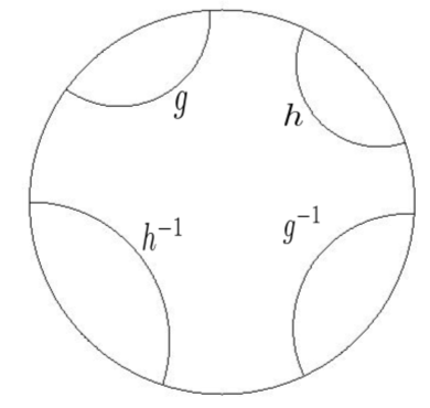
(a) A fundamental domain of the action of $\langle g,h\rangle$ on the Poincaré disc model.

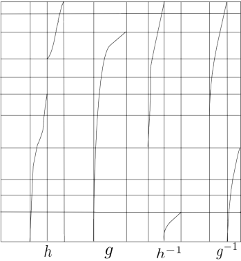
(b) The corresponding Bowen-Series map.

Figure 2.1. Example of a Fuchsian group.

Next we consider the corresponding shift space. Consider the alphabet $\underline{N}=\left\{0,\dots,N-1\right\}$. The limit set $X$ is then homeomorphic (mod $\nu$) to the set of all admissible words

$$\Sigma_{A}:=\{\omega=(\omega_{0},\omega_{1},\dots)\in\underline{N}^{\mathbb{N}}:\,A_{\omega_{i}\omega_{i+1}}=1\,\forall i\geq 0\}.$$

The homeomorphism is given, for $x\in X$, by

(2.1) $$\begin{array}[]{ll}\pi:&\Sigma_{A}\rightarrow X\\ &\omega\mapsto\lim_{n\rightarrow\infty}\tau_{\omega_{0}}\circ\dots\circ\tau_{\omega_{n}}(x),\end{array}$$

which is independent of the particular choice of $x\in X$.

Remark 2.4.

Furthermore, we define the cylinder sets for $\omega_{0},\dots,\omega_{k}\in\underline{N}$, $k\in\mathbb{N}_{0}$, as

$$\left[\omega_{0}\dots\omega_{k}\right]:=\left\{\left(\omega_{0}^{\prime},\omega_{1}^{\prime},\dots\right)\in\Sigma_{A}:\,\omega_{i}=\omega_{i}^{\prime},\,i\in\{0,\dots,k\}\right\}.$$

If for some $i\in\{0,\dots,k-1\}$ $A_{\omega_{i}\omega_{i+1}}=0$ then $\left[\omega_{0}\dots\omega_{k}\right]=\varnothing$.

Then the sets $B_{i}$ and $F\left(B_{i}\right)$ for $i\in\underline{N}$ are homeomorphic (mod $\nu$) to the following sets in the shift space:

$$\pi^{-1}\left(B_{i}\right)=[i]$$

and

$$\pi^{-1}\left(F(B_{i})\right)=\{\omega=\left(\omega_{0},\omega_{1},\dots\right)\in\Sigma_{A}:\,A_{i\omega_{0}}=1\}.$$

The dynamic of $F$ is conjugated to the shift dynamic $\sigma:\,\Sigma_{A}\rightarrow\Sigma_{A}$, $\sigma\left(\omega_{0},\omega_{1},\dots\right)=\left(\omega_{1},\omega_{2},\dots\right)$ and consequently, the functions $\tau_{i}$ correspond to the inverse branches of the shift function, i.e. $\tau_{i}\circ\pi\left(\omega_{0},\omega_{1},\dots\right)=\pi\left(i,\omega_{0},\omega_{1},\dots\right)$, for $\omega\in\pi^{-1}\left(F(B_{i})\right)$, $i\in\underline{N}$.

Furthermore, let us fix the following notation.

• $\Sigma_{A}^{n}:=\left\{\omega=\left(\omega_{0},\dots,\omega_{n-1}\right)\in\underline{N}^{n}:\text{ }A_{\omega_{i}\omega_{i+1}}=1\text{ for all }i\in\{0,\dots,n-1\}\right\}$ defines the set of admissible words of length $n\in\mathbb{N}$.

• $\Sigma_{A}^{*}$ stands for all finite words, i.e. $\Sigma_{A}^{*}=\bigcup_{n\geq 1}\Sigma_{A}^{n}$.

• For $\omega\in\Sigma_{A}^{n}$ we define $\tau_{\omega}:=\tau_{\omega_{0}}\circ\tau_{\omega_{1}}\circ\dots\circ\tau_{\omega_{n-1}}$.

• For $\omega\in\Sigma_{A}^{n}$, $\tau\in\Sigma_{A}^{m}$ we define their concatenation

  $$\omega\tau:=\left(\omega_{0},\dots,\omega_{n-1},\tau_{0},\dots,\tau_{m-1}\right)$$

  which is an element of $\Sigma_{A}^{n+m}$ whenever $A_{\omega_{n-1}\tau_{0}}=1$.

As a measure on $X$ we could consider for instance the pull-back under $\pi$ of Gibbs measures on $\Sigma_{A}$ (for definitions see e.g. [KS10]).

Now we define the appropriate space for which we want to construct a wavelet basis.

Definition 2.5.

Let $\widetilde{\nu}$ be a probability measure on $\left(\Sigma_{A},\mathcal{B}\right)$ and $\nu=\widetilde{\nu}\circ\pi^{-1}$. Define the enlarged fractal by

$$R=\bigcup_{k\in\mathbb{Z}}X+k$$

and define the $\mathbb{Z}$-convolution $\nu_{\mathbb{Z}}$ of the measure $\nu$ for a Borel set $B$ by

$$\nu_{\mathbb{Z}}(B)=\sum_{k\in\mathbb{Z}}\nu(B-k),$$

which clearly is an invariant measure under $\mathbb{Z}$-translation.

Remark 2.6.

One example is the space $L^{2}\left(\Sigma_{A},\mu_{\phi}\right)$, where $\Sigma_{A}$ denotes a one-sided topologically exact subshift of finite type. An important class of measures on $\Sigma_{A}$ are given by invariant Gibbs measure with respect to a Hölder continuous potential $\phi\in C\left(\Sigma_{A},\mathbb{R}\right)$, denoted by $\mu_{\phi}$, compare [KS10]. $\mu_{\phi}$ corresponds to the measure $\widetilde{\nu}$ in Definition 2.5.

In the following we use the convention $0^{-1}\cdot\mathbbm{1}_{\varnothing}=0$. For simplicity we let $\left[\omega_{0},\dots,\omega_{n-1}\right]$ also denote the sets $\tau_{\omega_{0}}\circ\dots\circ\tau_{\omega_{n-1}}(X)$ using the identification by $\pi$. Furthermore, in Section 4 the measure $\nu$ supported on $[0,1]$ always corresponds to a measure $\widetilde{\nu}$ on $\Sigma_{A}$ by $\nu=\widetilde{\nu}\circ\pi^{-1}$ and $\nu_{\mathbb{Z}}$ denotes the measure obtained from $\nu$ by $\mathbb{Z}$-convolution.

3. Abstract Multiresolution analysis

In this section we give a proof of Theorem 1.6. To do so we first construct mother wavelets explicitly and in the next step we prove that these give indeed an orthonormal basis. In this section we fix $\left(\mu,\left(\mathcal{U}^{(n)}\right)_{n\in\mathbb{Z}},\mathcal{T}\right)$ which allows a two-sided MRA.

For the construction of an ONB we cannot define the mother wavelets in terms of filter functions due to the fact that we have more than one father wavelet.

Remark 3.1.

If we have the usual setting from the literature, compare e.g. [Dau92], then we have a multiplicative MRA with a unitary operator $\mathcal{U}$ and the operator $T$ given in (1.2). In this case there is only one father wavelet $\varphi$ and there exists a so-called low-pass filter $m_{0}:\,\mathbb{T}\rightarrow\mathbb{T}$ of the form $m_{0}(z)=\sum_{k\in\mathbb{Z}}a_{k}z^{k}$, $a_{k}\in\mathbb{C}$, such that $\varphi=\mathcal{U}m_{0}(T)\varphi$. For the construction of the mother wavelets we look for $N-1$ high-pass filters $m_{j}:\mathbb{T}\rightarrow\mathbb{T}$ of the form $m_{j}:z\mapsto\sum_{k\in\mathbb{Z}}b_{k}^{j}z^{k}$, $b_{k}^{j}\in\mathbb{C}$, $j\in\underline{N}\backslash\{0\}$, where $N\in\mathbb{N}$ is connected to the scaling since it indicates on which interval $[0,N]$ the unit interval is mapped when the operator $\mathcal{U}$ is applied to $\mathbbm{1}_{[0,1]}$. The high-pass filters are chosen, such that the matrix

$$M(z):=\frac{1}{\sqrt{N}}\left(m_{j}(\rho^{l}z)\right)_{j,l\in\underline{N}},$$

where $\rho=e^{2\pi i/N}$, is unitary for almost all $z\in\mathbb{T}$. In terms of these high-pass filters the mother wavelets are defined as $\psi_{j}=\mathcal{U}m_{j}(T)\varphi$, $j\in\underline{N}\backslash\{0\}$.

We first notice that for $n\in\mathbb{N}$

(3.1) $$\left\{\left(l,j\right)\in\underline{N^{n}}\times\underline{N}\right\}=\left\{\left(\Big{\lfloor}\frac{k}{N}\Big{\rfloor},(k)_{N}\right):k\in\underline{N^{n+1}}\right\},$$

where $(m)_{N}:=m\mod N$ and $\lfloor x\rfloor=\max_{k\in\mathbb{Z},k\leq x}(k)$ is the largest integer not exceeding $x$.

Clearly from the definition of the MRA, Definition 1.4 (1e), we have the following:

1. If for $n\in\mathbb{N}_{0}$, $k\in\underline{N^{n+1}}$, $\mathcal{U}^{(n)}\mathcal{T}^{\lfloor\frac{k}{N}\rfloor}\varphi_{(k)_{N}}\neq 0$ , there exists uniquely determined $\left(a_{m}^{n,k}\right)_{m\in\underline{N^{n+2}}}\in\mathbb{C}^{N^{n+2}}$ such that

   (3.2) $$\begin{array}[]{cc}&\mathcal{U}^{(n)}\mathcal{T}^{\lfloor\frac{k}{N}\rfloor}\varphi_{(k)_{N}}=\mathcal{U}^{(n+1)}\sum_{m\in\underline{N^{n+2}}}a_{m}^{n,k}\mathcal{T}^{\lfloor\frac{m}{N}\rfloor}\varphi_{(m)_{N}}\\ \text{and }\\ &\left(a_{m}^{n,k}=0,\ m\in\underline{N^{n+2}},\ \text{ if }\mathcal{U}^{(n+1)}\mathcal{T}^{\lfloor\frac{m}{N}\rfloor}\varphi_{(m)_{N}}=0\right).\end{array}$$

2. If $\mathcal{U}^{(-n)}\varphi_{i}\neq 0$, $n\in\mathbb{N}$, $i\in\underline{N}$, there exists uniquely determined coefficients $\left(b_{m}^{n,i}\right)_{m\in\underline{N^{2}}}\in\mathbb{C}^{N^{2}}$ such that

   (3.3) $$\begin{array}[]{cc}&\mathcal{U}^{(-n)}\varphi_{i}=\mathcal{U}^{(-n+1)}\sum_{m\in\underline{N^{2}}}b_{m}^{n,i}\mathcal{T}^{\lfloor\frac{m}{N}\rfloor}\varphi_{(m)_{N}}\\ \text{ and }\\ &\left(b_{m}^{n,i}=0,\ m\in\underline{N^{2}},\ \text{ if }\mathcal{U}^{(-n+1)}\mathcal{T}^{\lfloor\frac{m}{N}\rfloor}\varphi_{(m)_{N}}=0\right).\end{array}$$

Remark 3.2.

We only consider $\mathcal{U}^{-(n)}\varphi_{i}$, since $\mathcal{U}^{(-n)}\mathcal{T}^{k}\varphi_{i}=\mathcal{T}^{N^{n}k}\mathcal{U}^{(-n)}\varphi_{i}$ by (1f) of Definition 1.4.

Lemma 3.3.

The following holds for the coefficients $\left(a_{m}^{n,k}\right)_{m\in\underline{N^{n+2}}}$, $k\in\underline{N^{n+1}}$, $n\in\mathbb{N}_{0}$, and $\left(b_{m}^{n,i}\right)_{m\in\underline{N^{2}}}$, $i\in\underline{N}$, $n\in\mathbb{N}$.

1. For fixed $n\in\mathbb{N}_{0}$, define

   (3.4) $$Q_{n}:=\left\{m\in\underline{N^{n+1}}:\mathcal{U}^{(n)}\mathcal{T}^{\lfloor\frac{m}{N}\rfloor}\varphi_{(m)_{N}}\neq 0\right\}.$$

   Then the vectors $v_{k}=\left(a_{m}^{n,k}\right)_{m\in\underline{N^{n+2}}}$, $k\in Q_{n}$, are orthonormal.

2. For fixed $n\in\mathbb{N}$, define

   (3.5) $$Q_{-n}:=\left\{m\in\underline{N}:\mathcal{U}^{(-n)}\varphi_{m}\neq 0\right\}.$$

   Then the vectors $w_{i}=\left(b_{m}^{n,i}\right)_{m\in\underline{N^{2}}}$, $i\in Q_{-n}$, are orthonormal.

Proof.

ad (1): For fixed $n\in\mathbb{N}_{0}$, let $k,l\in Q_{n}$, then

$$\delta_{(k,l)} =\langle\mathcal{U}^{(n)}\mathcal{T}^{\lfloor\frac{k}{N}\rfloor}\varphi_{(k)_{N}}|\mathcal{U}^{(n)}\mathcal{T}^{\lfloor\frac{l}{N}\rfloor}\varphi_{(l)_{N}}\rangle$$

$$=\big{\langle}\mathcal{U}^{(n+1)}\sum_{m\in\underline{N^{n+2}}}a_{m}^{n,k}\mathcal{T}^{\lfloor\frac{m}{N}\rfloor}\varphi_{(m)_{N}}\big{|}\mathcal{U}^{(n+1)}\sum_{m\in\underline{N^{n+2}}}a_{m}^{n,l}\mathcal{T}^{\lfloor\frac{m}{N}\rfloor}\varphi_{(m)_{N}}\big{\rangle}$$

$$=\sum_{m\in\underline{N^{n+2}}}a_{m}^{n,k}\overline{a}_{m}^{n,l}.$$

ad (2): Follows analogously to (1). ∎

3.1. Proof of Theorem 1.6

The aim is to prove the existence of a basis as given in Theorem 1.6. For this we divide the proof in two parts. First we construct coefficients such that the functions $\psi_{n,k}$ given in (3.6) and (3.7) give an orthonormal basis. In the second part we verify that these functions give indeed an orthonormal basis. We prove these parts first for $n\in\mathbb{N}_{0}$ and then for $n\in\mathbb{Z}$, $n<0$. We define the mother wavelets for each scale $n\in\mathbb{Z}$ such that we obtain with their translates a basis for $W_{n}=V_{n+1}\ominus V_{n}$, where $V_{n}$ is given in Definition 1.4 (1d). Define for $n\in\mathbb{N}_{0}$

$$D_{n} :=\left\{m\in\underline{N^{n+2}}:a_{m}^{n,k}\neq 0\text{ for some }k\in Q_{n}\right\},$$

$$D_{-n} :=\left\{m\in\underline{N^{2}}:b_{m}^{n,k}\neq 0\text{ for some }k\in Q_{-n}\right\},$$

and $d_{n}:=\operatorname{card}D_{n}$, $d_{-n}:=\operatorname{card}D_{-n}$.

• The mother wavelets for the subspaces $W_{n}$, $n\in\mathbb{N}_{0}$, of the MRA shall have the form for $k\in\underline{d_{n}-q_{n}}$ with $q_{n}:=\operatorname{card}Q_{n}$

  (3.6) $$\psi_{n,k}:=\mathcal{U}^{(n+1)}\sum_{m\in\underline{N^{n+2}}}c_{m}^{n,k}\mathcal{T}^{\lfloor\frac{m}{N}\rfloor}\varphi_{(m)_{N}},$$

  where the coefficients $c_{m}^{n,k}\in\mathbb{C}$ are given in (3.8).

• For the negative index subspaces $W_{-n}$, $n\in\mathbb{N}$, of $L^{2}(\mu)$ we define the mother wavelets in terms of the coefficients of the matrix in (3.9) for $n\in\mathbb{N}$ and $k\in\underline{d_{-n}-q_{-n}}$, where $q_{-n}:=\operatorname{card}Q_{-n}$, as

  (3.7) $$\psi_{-n,k}:=\mathcal{U}^{(-n+1)}\sum_{m\in\underline{N^{2}}}c_{m}^{-n,k}\mathcal{T}^{\lfloor\frac{m}{N}\rfloor}\varphi_{(m)_{N}}.$$

The coefficients $c_{m}^{n,k}\in\mathbb{C}$, $c_{m}^{-n,k}\in\mathbb{C}$ are determined in the following via the Gram-Schmidt process.

For the definition of the basis we fix $n\in\mathbb{N}_{0}$ and we construct an orthonormal basis for $\mathbb{C}^{d_{n}}$ in the following way. Consider $\left(a_{m}^{n,k}\right)_{k\in Q_{n},m\in D_{n}}$. This is a $\left(q_{n}\times d_{n}\right)$-matrix.

Now we consider $d_{n}-q_{n}$ vectors $e_{i}$, $i\in\underline{d_{n}-q_{n}},$ of length $d_{n}$ which are linearly independent of the vectors $\left(a_{m}^{n,k}\right)_{m\in D_{n}}$, $k\in Q_{n}$. Via the Gram-Schmidt process we obtain $d_{n}-q_{n}$ orthonormal vectors $\left(c_{m}^{n,i}\right)_{m\in D_{n}}$, $i\in\underline{d_{n}-q_{n}}$, of length $d_{n}$ which are orthonormal to $\left(a_{m}^{n,k}\right)_{m\in D_{n}}$, $k\in Q_{n}$. We extend the vectors $\left(c_{m}^{n,i}\right)_{m\in D_{n}}$ to some of length $\underline{N^{n+2}}$ by $c_{m}^{n,i}=0$ if $m\in\underline{N^{n+2}}\backslash D_{n}$ and we define a matrix $\mathcal{C}{}_{n}:=\left(c_{m}^{n,k}\right)_{k\in\underline{d_{n}-q_{n}},m\in\underline{N^{n+2}}}$ of size $\left(d_{n}-q_{n}\right)\times N^{n+2}$ and $\mathcal{A}{}_{n}:=\left(a_{m}^{n,k}\right)_{k\in Q_{n},m\in\underline{N^{n+2}}}$ of size $q_{n}\times N^{n+2}$. So we obtain a matrix of size $d_{n}\times N^{n+2}$ by

(3.8) $$\mathcal{M}{}_{n}:=\left(\begin{array}[]{c}\mathcal{A}{}_{n}\\ \mathcal{C}{}_{n}\end{array}\right).$$

Now we turn to the construction of the coefficients for $\psi_{-n,k}$, $n\in\mathbb{N}$, in (3.7). For each $-n$, $n\in\mathbb{N}$, we define an orthonormal basis of $\mathbb{C}^{d_{-n}}$ in the following way. Consider $\left(b_{m}^{n,k}\right)_{k\in Q_{-n},m\in D_{-n}}$. This is a $\left(q_{-n}\times d_{-n}\right)$-matrix. Now we consider $d_{-n}-q_{-n}$ vectors which are linearly independent of $\left(b_{m}^{n,k}\right)_{m\in D_{-n}}$. Via the Gram-Schmidt process we obtain $d_{-n}-q_{-n}$ orthonormal vectors $\left(c_{m}^{-n,j}\right)_{m\in D_{-n}}$, $j\in\underline{d_{-n}-q_{-n}}$, of length $d_{-n}$ which are orthonormal to $\left(b_{m}^{n,i}\right)_{m\in D_{-n}}$. In the last step we extend the vectors $\left(c_{m}^{-n,i}\right)_{m\in D_{-n}}$ to some of length $N^{2}$ by defining $c_{m}^{-n,i}=0$ if $m\in\underline{N^{2}}\backslash D_{-n}$. Now we define $\mathcal{D}{}_{n}:=\left(c_{m}^{-n,i}\right)_{i\in\underline{d_{-n}-q_{-n}},m\in\underline{N^{2}}}$ and $\mathcal{B}{}_{n}:=\left(b_{m}^{n,k}\right)_{k\in Q_{-n},m\in\underline{N^{2}}}$ such that

(3.9) $$\widetilde{\mathcal{M}}{}_{n}:=\left(\begin{array}[]{c}\mathcal{B}{}_{n}\\ \mathcal{D}{}_{n}\end{array}\right)$$

is a matrix of size $d_{-n}\times N^{2}$.

In the next step we show that we obtain indeed an orthonormal basis with these mother wavelets given in (3.6) and (3.7). First we prove this for $n\in\mathbb{N}_{0}$. Recall that $W_{n}=V_{n+1}\ominus V_{n}$ for $n\in\mathbb{N}_{0}$. Consequently, $\operatorname{cl}\left(\bigcup_{n\in\mathbb{N}_{0}}W_{n}\cup V_{0}\right)=L^{2}(\mu)$ since for every $n\in\mathbb{N}_{0}$ it follows iteratively that $V_{n+1}=\bigoplus_{k=0}^{n}W_{k}\oplus V_{0}$. Now we show that for fixed $n\in\mathbb{N}$ we have that $\left\{\mathcal{T}^{l}\psi_{n,k}:k\in\underline{d_{n}-q_{n}},l\in\mathbb{Z}\right\}$ is an orthonormal basis of $W_{n}$. First we show the orthonormality.

To show the orthonormality of $\mathcal{T}^{r}\psi_{n,k}$ and $\mathcal{T}^{s}\psi_{n,l}$, $r,s\in\mathbb{Z}$, $k,l\in\underline{d_{n}-q_{n}}$, it is sufficient to consider $\mathcal{T}^{r}\psi_{n,k}$ and $\psi_{n,l}$ since the operator $\mathcal{T}$ is unitary. The orthonormality follows then from

$$\langle\mathcal{T}^{r}\psi_{n,k}|\psi_{n,l}\rangle =\Big{\langle}\sum_{m\in\underline{N^{n+2}}}c_{m}^{n,k}\mathcal{U}^{(n+1)}\mathcal{T}^{\lfloor\frac{m}{N}\rfloor+N^{n+1}r}\varphi_{(m)_{N}}\Big{|}\sum_{m\in\underline{N^{n+2}}}c_{m}^{n,l}\mathcal{U}^{(n+1)}\mathcal{T}^{\lfloor\frac{m}{N}\rfloor}\varphi_{(m)_{N}}\Big{\rangle}$$

$$=\Big{\langle}\sum_{m\in\underline{N^{n+2}}}c_{m}^{n,k}\mathcal{T}^{\lfloor\frac{m}{N}\rfloor+N^{n+1}r}\varphi_{(m)_{N}}\Big{|}\sum_{m\in\underline{N^{n+2}}}c_{m}^{n,l}\mathcal{T}^{\lfloor\frac{m}{N}\rfloor}\varphi_{(m)_{N}}\Big{\rangle}$$

$$=\sum_{m\in\underline{N^{n+2}}}\sum_{s\in\underline{N^{n+2}}}c_{m}^{n,k}\overline{c}_{s}^{n,l}\Big{\langle}\mathcal{T}^{N^{n+1}r+\lfloor\frac{m}{N}\rfloor}\varphi_{(m)_{N}}\Big{|}\mathcal{T}^{\lfloor\frac{s}{N}\rfloor}\varphi_{(s)_{N}}\Big{\rangle}$$

$$=\sum_{m\in\underline{N^{n+2}}}\sum_{s\in\underline{N^{n+2}}}c_{m}^{n,k}\overline{c}_{s}^{n,l}\cdot\delta_{(N^{n+1}r+\lfloor\frac{m}{N}\rfloor,\lfloor\frac{s}{N}\rfloor),((m)_{N},(s)_{N})}$$

$$=\delta_{r,0}\cdot\sum_{m\in\underline{N^{n+2}}}c_{m}^{n,k}\overline{c}_{m}^{n,l}$$

$$=\delta_{r,0}\cdot\delta_{k,l}.$$

In the next step we show that $V_{n+1}=V_{n}\oplus W_{n}$. We consider a basis element of $V_{n+1}$ of the form $\mathcal{U}^{(n+1)}\mathcal{T}^{\lfloor\frac{k}{N}\rfloor}\varphi_{(k)_{N}}$, $k\in\underline{N^{n+2}}$, and show that it is a linear combination of functions $\mathcal{U}^{(n)}\mathcal{T}^{\lfloor\frac{l}{N}\rfloor}\varphi_{(l)_{N}}$ and $\psi_{n,m}$, $l\in\underline{N^{n+1}}$, $m\in\underline{d_{n}-q_{n}}$. It is sufficient to consider only $k\in\underline{N^{n+2}}$ by Definition 1.4 (1e). If $\mathcal{U}^{(n+1)}\mathcal{T}^{\lfloor\frac{k}{N}\rfloor}\varphi_{(k)_{N}}=0$ it is obvious satisfied. If $\mathcal{U}^{(n+1)}\mathcal{T}^{\lfloor\frac{k}{N}\rfloor}\varphi_{(k)_{N}}\neq 0$, $k\in\underline{N^{n+2}}$, it can be written as the following linear combination:

$$\mathcal{U}^{(n+1)}\mathcal{T}^{\lfloor\frac{k}{N}\rfloor}\varphi_{(k)_{N}}$$

$$= \mathcal{U}^{(n+1)}\left(\sum_{m\in\underline{N^{n+2}}}\underbrace{\left(\sum_{l\in Q_{n}}\overline{a}_{k}^{n,l}a_{m}^{n,l}+\sum_{l\in\underline{d_{n}-q_{n}}}\overline{c}_{k}^{n,l}c_{m}^{n,l}\right)}_{=\delta_{k,m}}\mathcal{T}^{\lfloor\frac{m}{N}\rfloor}\varphi_{(m)_{N}}\right)$$

$$= \mathcal{U}^{(n+1)}\left(\sum_{l\in Q_{n}}\overline{a}_{k}^{n,l}\sum_{m\in\underline{N^{n+2}}}a_{m}^{n,l}\mathcal{T}^{\lfloor\frac{m}{N}\rfloor}\varphi_{(m)_{N}}+\sum_{l\in\underline{d_{n}-q_{n}}}\overline{c}_{k}^{n,l}\sum_{m\in\underline{N^{n+2}}}c_{m}^{n,l}\mathcal{T}^{\lfloor\frac{m}{N}\rfloor}\varphi_{(m)_{N}}\right)$$

$$= \sum_{l\in Q_{n}}\overline{a}_{k}^{n,l}\mathcal{U}^{(n)}\mathcal{T}^{\lfloor\frac{l}{N}\rfloor}\varphi_{(l)_{N}}+\sum_{l\in\underline{d_{n}-q_{n}}}\overline{c}_{k}^{n,l}\mathcal{U}^{(n+1)}\sum_{m\in\underline{N^{n+2}}}c_{m}^{n,l}\mathcal{T}^{\lfloor\frac{m}{N}\rfloor}\varphi_{(m)_{N}}$$

$$= \sum_{l\in Q_{n}}\overline{a}_{k}^{n,l}\mathcal{U}^{(n)}T^{\lfloor\frac{l}{N}\rfloor}\varphi_{(l)_{N}}+\sum_{l\in\underline{d_{n}-q_{n}}}\overline{c}_{k}^{n,l}\psi_{n,l}.$$

If we consider $\mathcal{T}^{l}\psi_{n,k}$ and $\mathcal{T}^{r}\psi_{m,s}$ for $n,m\in\mathbb{N}$, $n\neq m$, $l,r\in\mathbb{Z}$, $k\in\underline{d_{n}-q_{n}}$, $s\in\underline{d_{m}-q_{m}}$, the orthonormality follows from $\mathcal{T}^{l}\psi_{n,k}\in W_{n}$, $\mathcal{T}^{r}\psi_{m,s}\in W_{m}$ and by the definition of $W_{n}$, $W_{m}$.

Now we consider the closed subspaces $V_{n}$ of $L^{2}(\mu)$ with $n<0$ and show the analogous results. We show that for fixed $n\in\mathbb{N}$ $\left\{\mathcal{T}^{N^{n}k}\psi_{-n,l}:\,l\in\underline{d_{-n}-q_{-n}},\,k\in\mathbb{Z}\right\}$ is an orthonormal basis of $W_{-n}=V_{-n+1}\ominus V_{-n}$. First we show that any function $\mathcal{U}^{(-n+1)}\varphi_{j}$ can be written as a linear combination of functions $\mathcal{U}^{(-n)}\varphi_{i}$ and $\psi_{-n,l}$, $i\in\underline{N}$, $l\in\underline{d_{-n}-q_{-n}}$. This linear combination is precisely

$$\mathcal{U}^{(-n+1)}\varphi_{j}$$

$$= \mathcal{U}^{(-n+1)}\left(\sum_{m\in\underline{N^{2}}}\left(\underbrace{\sum_{i\in Q_{-n}}\overline{b}_{j}^{n,i}b_{m}^{n,i}+\sum_{l\in\underline{d_{-n}-q_{-n}}}\overline{c}_{j}^{-n,l}c_{m}^{-n,l}}_{=\delta_{j,m}}\right)\mathcal{T}^{\lfloor\frac{m}{N}\rfloor}\varphi_{(m)_{N}}\right)$$

$$= \mathcal{U}^{(-n+1)}\left(\sum_{i\in Q_{-n}}\overline{b}_{j}^{n,i}\sum_{m\in\underline{N^{2}}}b_{m}^{n,i}\mathcal{T}^{\lfloor\frac{m}{N}\rfloor}\varphi_{(m)_{N}}+\sum_{m\in\underline{N^{2}}}\sum_{l\in\underline{d_{-n}-q_{-n}}}\overline{c}_{j}^{-n,l}c_{m}^{-n,l}\mathcal{T}^{\lfloor\frac{m}{N}\rfloor}\varphi_{(m)_{N}}\right)$$

$$= \sum_{i\in Q_{-n}}\overline{b}_{j}^{n,i}\mathcal{U}^{(-n)}\varphi_{i}+\sum_{l\in\underline{d_{-n}-q_{-n}}}\overline{c}_{j}^{-n,l}\mathcal{U}^{(-n+1)}\sum_{m\in\underline{N^{2}}}c_{m}^{-n,l}\mathcal{T}^{\lfloor\frac{m}{N}\rfloor}\varphi_{(m)_{N}}$$

$$= \sum_{i\in Q_{-n}}\overline{b}_{j}^{n,i}\mathcal{U}^{(-n)}\varphi_{i}+\sum_{l\in\underline{d_{-n}-q_{-n}}}\overline{c}_{j}^{-n,l}\psi_{-n,l}.$$

We have to show the orthonormality only for $\psi_{-n,l}$ and $\psi_{-n,k}$ since $\mathcal{T}$ is a unitary operator and $\mathcal{U}^{(-n+1)}\mathcal{T}^{k}\varphi_{j}$ are mapped to orthonormal functions. For $\psi_{-n,l}$ and $\psi_{-n,k}$, $l,k\in\underline{d_{-n}-q_{-n}}$, the orthonormality follows from

$$\langle\psi_{-n,l}|\psi_{-n,k}\rangle =\Big{\langle}\sum_{m\in\underline{N^{2}}}c_{m}^{-n,l}\mathcal{U}^{(-n+1)}\mathcal{T}^{\lfloor\frac{m}{N}\rfloor}\varphi_{(m)_{N}}\Big{|}\sum_{m\in\underline{N}^{2}}c_{m}^{-n,k}\mathcal{U}^{(-n+1)}\mathcal{T}^{\lfloor\frac{m}{N}\rfloor}\varphi_{(m)_{N}}\Big{\rangle}$$

$$=\sum_{m\in\underline{N^{2}}}c_{m}^{-n,l}\overline{c}_{m}^{-n,k}$$

$$=\delta_{l,k}.$$

Furthermore, it follows that $L^{2}(\mu)=\bigoplus_{k\in\mathbb{Z}}W_{k}$, since we have shown before that $\operatorname{cl}\left(\bigcup_{n\in\mathbb{N}_{0}}W_{n}\cup V_{0}\right)=L^{2}(\mu)$. Consequently, we have that

$$\left\{\mathcal{T}^{l}\psi_{n,k}:n\in\mathbb{Z},k\in\underline{d_{n}-q_{n}},l\in\mathbb{Z}\right\}$$

is an ONB of $L^{2}(\mu)$.

Remark 3.4.

For the proof of Corollary 1.8 we have to consider the first part of the proof of Theorem 1.6 and show the orthonormality between $\psi_{n,k}$ and $\varphi_{i}$ in addition, which follows from the construction of the mother wavelets.

3.2. Abstract multiplicative Multiresolution analysis

In this section we want to consider how the general results simplify if we impose the extra condition of a multiplicative MRA.

Recall from the introduction that in the case of Definition 1.4, we say that we have a multiplicative MRA if there exists an operator $\mathcal{U}$ such that $\mathcal{U}^{(n)}=\mathcal{U}^{n}$ for all $n\in\mathbb{N}$ and $\mathcal{U}^{(-n)}=\left(\mathcal{U}^{*}\right)^{n}$, $n\in\mathbb{N}$. We then say $\left(\mu,\left(\left(\mathcal{U}\right)^{n},\left(\mathcal{U}^{*}\right)^{n}\right)_{n\in\mathbb{N}_{0}},\mathcal{T}\right)$ allows a two-sided multiplicative MRA.

The key observation is contained in Lemma 1.9 which we prove first.

Proof of Lemma 1.9.

Recall that $\left\{\mathcal{T}^{l}\psi_{0,k}:k\in\underline{d_{0}-N},\ l\in\mathbb{Z}\right\}$ is an orthonormal basis of $W_{0}$. We have $\psi_{0,k}=\sum_{m\in\underline{N^{2}}}c_{m}^{0,k}\mathcal{U}\mathcal{T}^{\lfloor\frac{m}{N}\rfloor}\varphi_{(m)_{N}}$ and we show that for fixed $n\in\mathbb{N}$, $\mathcal{U}^{n}W_{0}=W_{n}$. First it follows that $\mathcal{U}^{n}\mathcal{T}^{m}\psi_{0,k}\in W_{n}\subset V_{n+1}$, $n\in\mathbb{N}$, $m\in\mathbb{Z}$, since

$$\mathcal{U}^{n}\mathcal{T}^{m}\psi_{0,k}=\sum_{l\in\underline{N^{2}}}c_{l}^{0,k}\mathcal{U}^{n+1}\mathcal{T}{}^{\lfloor\frac{l}{N}\rfloor+Nm}\varphi_{(l)_{N}}$$

and

$$\langle\mathcal{U}^{n}\mathcal{T}^{m}\psi_{0,k}|\mathcal{U}^{n}\mathcal{T}^{r}\varphi_{i}\rangle$$

$$= \langle\mathcal{U}^{n}\mathcal{T}^{m}\sum_{l\in\underline{N^{2}}}c_{l}^{0,k}\mathcal{U}\mathcal{T}^{\lfloor\frac{l}{N}\rfloor}\varphi_{(l)_{N}}|\mathcal{U}^{n}T^{r}\sum_{j\in\underline{N^{2}}}a_{j}^{0,i}\mathcal{U}\mathcal{T}^{\lfloor\frac{j}{N}\rfloor}\varphi_{(j)_{N}}\rangle$$

$$= \langle\mathcal{U}^{n+1}\mathcal{T}^{Nm}\sum_{l\in\underline{N^{2}}}c_{l}^{0,k}\mathcal{T}^{\lfloor\frac{l}{N}\rfloor}\varphi_{(l)_{N}}|\mathcal{U}^{n+1}\mathcal{T}^{Nr}\sum_{j\in\underline{N^{2}}}a_{j}^{0,i}\mathcal{T}^{\lfloor\frac{j}{N}\rfloor}\varphi_{(j)_{N}}\rangle$$

$$= \delta_{m,r}\cdot\sum_{l\in\underline{N^{2}}}c_{l}^{0,k}a_{l}^{0,i}=0.$$

Consequently, $\mathcal{U}^{n}W_{0}\subset W_{n}$. Now consider $\mathcal{U}^{n+1}\mathcal{T}^{m}\varphi_{j}\in V_{n+1}$, $m\in\mathbb{Z}$, $j\in\underline{N}$, and we show that this can be written as a linear combination of functions $\mathcal{U}^{n}\mathcal{T}^{l}\varphi_{i}$ and $\mathcal{U}^{n}\mathcal{T}^{r}\psi_{0,k}$, $l,r\in\mathbb{Z}$, $i\in\underline{N}$, $k\in\underline{d_{0}-N}$, by considering the scalar product. First we recall that $\mathcal{U}\mathcal{T}^{\lfloor\frac{k}{N}\rfloor}\varphi_{(k)_{N}}=\sum_{i\in\underline{N}}\overline{a}_{k}^{0,i}\varphi_{i}+\sum_{l\in\underline{d_{0}-N}}\overline{c}_{k}^{0,l}\psi_{0,l}$ for $k\in\underline{N^{2}}$ from the proof of Theorem 1.6, and hence for $k\in\underline{N^{2}}$

$$1 =\langle\mathcal{U}\mathcal{T}^{\lfloor\frac{k}{N}\rfloor}\varphi_{(k)_{N}}|\sum_{i\in\underline{N}}\overline{a}_{k}^{0,i}\varphi_{i}+\sum_{l\in\underline{d_{0}-N}}\overline{c}_{k}^{0,l}\psi_{0,l}\rangle$$

$$=\sum_{i\in\underline{N}}\overline{a}_{k}^{0,i}a_{k}^{0,i}+\sum_{l\in\underline{d_{0}-N}}\overline{c}_{k}^{0,l}c_{k}^{0,l}.$$

It follows that for $m\in\underline{N^{n+2}}$ with $m=k+N^{2}k_{1}$, $k\in\underline{N^{2}}$, $k_{1}\in\underline{N^{n}}$, we have $\lfloor\frac{m}{N}\rfloor=\lfloor\frac{k}{N}\rfloor+Nk_{1}$ and $(m)_{N}=(k)_{N}$, and so

$$\langle\mathcal{U}^{n+1}\mathcal{T}^{\lfloor\frac{k}{N}\rfloor+Nk_{1}}\varphi_{(k)_{N}}|\mathcal{U}^{n}\mathcal{T}^{k_{1}}\sum_{i\in\underline{N}}\overline{a}_{k}^{0,i}\varphi_{i}+\mathcal{U}^{n}\mathcal{T}^{k_{1}}\sum_{l\in\underline{d_{0}-N}}\overline{c}_{k}^{0,l}\psi_{0,l}\rangle$$

$$= \langle\mathcal{U}^{n+1}\mathcal{T}^{\lfloor\frac{k}{N}\rfloor+Nk_{1}}\varphi_{(k)_{N}}|\mathcal{U}^{n}\mathcal{T}^{k_{1}}\sum_{i\in\underline{N}}\overline{a}_{k}^{0,i}\sum_{l\in\underline{N^{2}}}a_{l}^{0,i}\mathcal{U}\mathcal{T}^{\lfloor\frac{l}{N}\rfloor}\varphi_{(l)_{N}}\rangle$$

$$+\langle\mathcal{U}^{n+1}\mathcal{T}^{\lfloor\frac{k}{N}\rfloor+Nk_{1}}\varphi_{(k)_{N}}|\mathcal{U}^{n}\mathcal{T}^{k_{1}}\sum_{l\in\underline{d_{0}-N}}\overline{c}_{k}^{0,l}\sum_{i\in\underline{N^{2}}}c_{i}^{0,l}\mathcal{U}\mathcal{T}^{\lfloor\frac{i}{N}\rfloor}\varphi_{(i)_{N}}\rangle$$

$$= \langle\mathcal{T}^{\lfloor\frac{k}{N}\rfloor+Nk_{1}}\varphi_{(k)_{N}}|\mathcal{T}^{Nk_{1}}\sum_{i\in\underline{N}}\overline{a}_{k}^{0,i}\sum_{l\in\underline{N^{2}}}a_{l}^{0,i}\mathcal{T}^{\lfloor\frac{l}{N}\rfloor}\varphi_{(l)_{N}}\rangle$$

$$+\langle\mathcal{T}^{\lfloor\frac{k}{N}\rfloor+Nk_{1}}\varphi_{(k)_{N}}|\mathcal{T}^{Nk_{1}}\sum_{l\in\underline{d_{0}-N}}\overline{c}_{k}^{0,l}\sum_{i\in\underline{N^{2}}}c_{i}^{0,l}\mathcal{T}^{\lfloor\frac{i}{N}\rfloor}\varphi_{(i)_{N}}\rangle$$

$$= \sum_{i\in\underline{N}}\overline{a}_{k}^{0,i}a_{k}^{0,i}+\sum_{l\in\underline{d_{0}-N}}\overline{c}_{k}^{0,l}c_{k}^{0,l}$$

$$= 1.$$

Now we notice that we can write any element $k\in\mathbb{Z}$ as $k=k_{0}+N^{n+2}l$ for some $k_{0}\in\underline{N^{n+2}}$ and $l\in\mathbb{Z}$. Consequently, with $\mathcal{U}\mathcal{T}^{N}|_{V_{0}}=\mathcal{T}\mathcal{U}|_{V_{0}}$ we obtain the general result for $\mathcal{U}^{n+1}\mathcal{T}^{k}\varphi_{j}$, $k\in\mathbb{Z}$, $j\in\underline{N}$.

To obtain $W_{-n}=\left(\mathcal{U}^{*}\right)^{n}W_{-1}$, $W_{-1}=V_{0}\ominus V_{-1}$, $n\in\mathbb{N}$, we can proceed as above. First we have from the proof of Theorem 1.6 that $\psi_{-1,k}=\sum_{l\in\underline{N^{2}}}c_{l}^{-1,k}\mathcal{T}^{\lfloor\frac{l}{N}\rfloor}\varphi_{(l)_{N}}$ and that $\varphi_{j}$, $j\in\underline{N}$, can be represented as $\varphi_{j}=\sum_{i\in\underline{N}}\overline{b}_{0,j}^{-1,i}\mathcal{U}^{*}\varphi_{i}+\sum_{l\in\underline{d_{-1}-N}}\overline{c}_{j}^{-1,l}\psi_{-1,l}$. With these observations we obtain as above that

$$\langle\left(\mathcal{U}^{*}\right)^{n}\mathcal{T}^{m}\varphi_{j}|\left(\mathcal{U}^{*}\right)^{n-1}\mathcal{T}^{r}\psi_{-1,k}\rangle=0$$

and

$$\langle\left(\mathcal{U}^{*}\right)^{n-1}\mathcal{T}^{k}\varphi_{j}|\left(\mathcal{U}^{*}\right)^{n}\sum_{i\in\underline{N}}\overline{b}_{j}^{-1,i}\varphi_{i}+\left(\mathcal{U}^{*}\right)^{n-1}\sum_{l\in\underline{d_{-1}-N}}\overline{c}_{j}^{-1,l}\psi_{-1,l}\rangle=1.$$

∎

Remark 3.5.

If we have $\mathcal{U}\mathcal{U}^{*}=\operatorname{id}$, then $W_{0}=\mathcal{U}\left(W_{-1}\right)$. Notice that $\mathcal{U}$ is not necessarily injective on $W_{-1}$.

Now we turn to the mother wavelets.

Remark 3.6.

If $\mathcal{U}^{(n)}=\mathcal{U}^{n}$, $\mathcal{U}^{(-n)}=\left(\mathcal{U}^{*}\right)^{n}$, then we only consider the mother wavelets for $k\in\underline{d_{0}-N}$. So

$$\psi_{0,k}=\mathcal{U}\sum_{l\in\underline{N^{2}}}c_{l}^{0,k}\mathcal{T}^{\lfloor\frac{l}{N}\rfloor}\varphi_{(l)_{N}},$$

where the coefficients are from (3.2) and we define $\psi_{k}:=\psi_{0,k}$.

For the negative indexed part of the construction we write for $k\in\underline{d_{-1}-N}$

$$\psi_{-,k}=\sum_{l\in\underline{N^{2}}}c_{l}^{-1,k}\mathcal{T}^{\lfloor\frac{l}{N}\rfloor}\varphi_{(l)_{N}}.$$

3.3. Translation completeness

In the following we assume a stronger condition than (1e) of Definition 1.4, namely that the father wavelets are translation complete, i.e. for $j\in\underline{N}$

(3.10) $$\varphi_{j}\in\operatorname{span}\mathcal{U}\left\{\mathcal{T}^{j}\varphi_{i}:i\in\underline{N}\right\}.$$

This condition implies that there exist complex numbers $a_{i}^{0,j}$, $i\in\underline{N}$, such that

$$\varphi_{j}=\sum_{i\in\underline{N}}a_{i}^{0,j}\mathcal{U}\mathcal{T}^{j}\varphi_{i}.$$

We would like to point out that this condition is also satisfied for the particular case of MIM where the father wavelets $\varphi_{j}$, $j\in\underline{N},$ are chosen to be the scaled characteristic functions on the cylinder sets $[j]$ (see Section 4).

We have that (3.2) takes the following form for $k\in\mathbb{Z}$, $j\in\underline{N}$, $n\in\mathbb{N}$,

$$\mathcal{U}^{n}\mathcal{T}^{k}\varphi_{j}=\sum_{l\in\underline{N^{2}}}a_{l}^{0,j}\mathcal{U}^{n+1}\mathcal{T}^{Nk+\lfloor\frac{l}{N}\rfloor}\varphi_{(l)_{N}}$$

and under condition (3.10) this simplifies to

$$\mathcal{U}^{n}\mathcal{T}^{k}\varphi_{j}=\sum_{i\in\underline{N}}a_{i}^{0,j}\mathcal{U}^{n+1}\mathcal{T}^{Nk+j}\varphi_{i}.$$

To simplify the notation we set $a_{l}^{j}:=a_{l}^{0,j}$. We now show that condition (3.10) allows us to simplify the construction of the mother wavelets.

Lemma 3.7.

Under condition (3.10) one possible choice of the matrix $\mathcal{M}{}_{0}$ in (3.8) has a block structure consisting of $N$ blocks.

Proof.

Define $Q^{k}:=\{j\in\underline{N}:\,\mathcal{U}\mathcal{T}^{k}\varphi_{j}\neq 0\}$ and $q^{k}:=\operatorname{card}Q^{k}$ for each $k\in\underline{N}$. Then $\left(a_{j}^{k}\right)_{j\in Q^{k}}$ is a vector of length $q^{k}$ and we choose $q^{k}-1$ linearly independent vectors to $\left(a_{j}^{k}\right)_{j\in Q^{k}}$ of length $q^{k}$. Via the Gram-Schmidt process we obtain vectors $\left(c_{j}^{k,l}\right)_{j\in Q^{k}}$, $l\in\underline{q^{k}}\backslash\{0\}$, orthonormal to $\left(a_{j}^{k}\right)_{j\in Q^{k}}$. By setting $c_{j}^{k,l}=0$ if $j\in\underline{N}\backslash Q^{k}$ we extend the vectors $\left(c_{j}^{k,l}\right)_{j\in Q^{k}}$ to $\left(c_{j}^{k,l}\right)_{j\in\underline{N}}$. Then $M_{k}:=\left(\begin{array}[]{c}\left(a_{j}^{k}\right)_{j\in\underline{N}}\\ \left(c_{j}^{k,l}\right)_{l\in\underline{q^{k}}\backslash\{0\},j\in\underline{N}}\end{array}\right)$ is a matrix of size $q^{k}\times N$.

The matrix $\widehat{\mathcal{M}}_{0}=\left(h_{ij}\right)_{i\in\underline{q_{1}},j\in\underline{N^{2}}}$ given with the blocks $M_{k}$, $k\in\underline{N}$, by for $k=0$

$$\left(h_{ij}\right)_{i\in\underline{q^{0}},j\in\underline{N}}=M_{0},$$

for $k\in\underline{N}\backslash\{0\}$

$$\left(h_{ij}\right)_{i\in\underline{\sum_{l=0}^{k}q^{l}}\backslash\underline{\sum_{l=0}^{k-1}q^{l}},j\in\underline{(k+1)N}\backslash\underline{kN}}=M_{k}$$

and otherwise zero satisfies the conditions imposed on $\mathcal{M}_{0}$ in (3.8), i.e. if we restrict the columns to those in $D_{1}$, it is unitary, and $\widehat{\mathcal{M}_{0}}$ is of size $q_{1}\times N^{2}$ since $\sum_{k\in\underline{N}}q^{k}=q_{1}$. We notice that $\widehat{\mathcal{M}}_{0}$ is ordered in a different way than $\mathcal{M}_{0}$, since the rows $\left(a_{j}^{k}\right)_{j\in Q^{k}}$ are not grouped in $\mathcal{M}_{0}$. ∎

Remark 3.8.

  

1. If $\mathcal{U}^{(n)}=\mathcal{U}^{n}$, $\mathcal{U}^{(-n)}=\left(\mathcal{U}^{*}\right)^{n}$ and (3.10), the mother wavelets take the simpler form for $k=0$, $l\in\underline{q^{0}}\backslash\{0\}$ and for $k\in\underline{N}\backslash\{0\}$, $l\in\underline{\sum_{i=0}^{k}q^{i}}\backslash\underline{\sum_{i=0}^{k-1}q^{i}}$, as

   $$\psi_{l}=\sum_{j\in\underline{N}}c_{j}^{k,l}\mathcal{U}\mathcal{T}^{k}\varphi_{j},$$

   where the coefficients are as constructed in Lemma 3.7. For negative indexed part we define for $k\in\underline{d_{-1}-N}$

   $$\psi_{-,k}=\sum_{l\in\underline{N^{2}}}c_{l}^{-1,k}\mathcal{T}^{\lfloor\frac{l}{N}\rfloor}\varphi_{(l)_{N}}.$$

2. In the case of (3.10), or the slightly weaker statement

   (3.11) $$\mathcal{U}^{(n)}\mathcal{T}^{\lfloor\frac{k}{N}\rfloor}\varphi_{(k)_{N}}=\sum_{i\in\underline{N}}a_{i}^{n,k}\mathcal{U}^{(n+1)}\mathcal{T}^{N\lfloor\frac{k}{N}\rfloor+(j)_{N}}\varphi_{i}$$

   we can obtain the coefficients for the mother wavelets by constructing for each $k\in\underline{N^{n}}$ with $\mathcal{U}^{(n)}\mathcal{T}^{k}\varphi_{j}\not\neq 0$ for at least one $j\in\underline{N}$ a matrix of size $q^{n,k}\times q^{n,k}$, where $q^{n,k}=\operatorname{card}\{j\in\underline{N}:\,\mathcal{U}^{(n)}\mathcal{T}^{k}\varphi_{j}\not\neq 0\}$ instead of one unitary matrix of size $d_{n}\times d_{n}$. In this way we need at most $N^{n}$ matrices on the scale $n\in\mathbb{N}$.

Now we turn to a correspondence to the construction of a wavelet basis for MIM. The next proposition shows how the incidence matrix of MIM plays a role in the MRA.

Proposition 3.9.

In the case of $\mathcal{U}^{(n)}=\left(\mathcal{U}^{(1)}\right)^{n}$, $n\in\mathbb{N}_{0}$, (3.10) and if it further holds that $a_{i}^{0,j}\neq 0$ if and only if $\mathcal{U}\mathcal{T}^{j}\varphi_{i}\neq 0$, $i,j\in\underline{N}$, then we have for $n\in\mathbb{N}$, $k\in\mathbb{Z}$, $\mathcal{U}^{n}\mathcal{T}^{k}\varphi_{j}\neq 0$ if and only if for all $i=0,\dots,n-2$, $\mathcal{U}\mathcal{T}^{k_{i+1}}\varphi_{k_{i}}\not\neq 0$ and $\mathcal{U}\mathcal{T}^{k_{0}}\varphi_{j}\neq 0$, where $k=\sum_{i=0}^{n-1}k_{i}N^{i}+lN^{n}$, $k_{i}\in\underline{N}$ , $i\in\underline{n}$, and $l\in\mathbb{Z}$.

Proof.

We prove this for $k=k_{0}+Nk_{1}$, $k_{0},k_{1}\in\underline{N}$. The general result follows iteratively. Notice that $\mathcal{U}^{2}\mathcal{T}^{k_{0}+Nk_{1}}\varphi_{j}=\mathcal{U}\mathcal{T}^{k_{1}}\left(\mathcal{U}\mathcal{T}^{k_{0}}\varphi_{j}\right)$. Consequently, from $\mathcal{U}^{2}\mathcal{T}^{k_{0}+Nk_{1}}\varphi_{j}\neq 0$ it follows that $\mathcal{U}\mathcal{T}^{k_{0}}\varphi_{j}\neq 0$. Besides we have that

$$\mathcal{U}\mathcal{T}^{k_{1}}\varphi_{k_{0}}=\mathcal{U}\mathcal{T}^{k_{1}}\sum_{i\in\underline{N}}a_{i}^{k_{0}}\mathcal{U}\mathcal{T}^{k_{0}}\varphi_{i}=\mathcal{U}^{2}\mathcal{T}^{Nk_{1}+k_{0}}\sum_{i\in\underline{N}}a_{i}^{k_{0}}\varphi_{i}\neq 0$$

if $\mathcal{U}^{2}\mathcal{T}^{k_{0}+Nk_{1}}\varphi_{j}\neq 0$.

If we assume that $\mathcal{U}\mathcal{T}^{k_{1}}\varphi_{k_{0}}\neq 0$ and $\mathcal{U}\mathcal{T}^{k_{0}}\varphi_{j}\neq 0$ then

$$\mathcal{U}^{2}\mathcal{T}^{Nk_{1}+k_{0}}\varphi_{j} =\mathcal{U}\mathcal{T}^{k_{1}}\mathcal{U}\mathcal{T}^{k_{0}}\varphi_{j}$$

$$=\left(a_{j}^{k_{0}}\right)^{-1}\mathcal{U}\mathcal{T}^{k_{1}}\left(\varphi_{k_{0}}-\sum_{i\in\underline{N}\backslash\{j\}}a_{i}^{k_{0}}\mathcal{U}\mathcal{T}^{k_{0}}\varphi_{i}\right)$$

$$=\left(a_{j}^{k_{0}}\right)^{-1}\left(\mathcal{U}\mathcal{T}^{k_{1}}\varphi_{k_{0}}-\sum_{i\in\underline{N}\backslash\{j\}}a_{i}^{k_{0}}\mathcal{U}^{2}\mathcal{T}^{Nk_{1}+k_{0}}\varphi_{i}\right)$$

$$\neq 0,$$

since $\mathcal{U}\mathcal{T}^{k_{1}}\varphi_{k_{0}}-\sum_{i\in\underline{N}\backslash\{j\}}a_{i}^{k_{0}}\mathcal{U}^{2}\mathcal{T}^{Nk_{1}+k_{0}}\varphi_{i}=a_{j}^{k_{0}}\mathcal{U}T^{Nk_{1}+k_{0}}\varphi_{j}\neq 0$.∎

Remark 3.10.

We can show the same result if for some $c\in\mathbb{R}$, we have $\mathcal{U}^{(n)}\mathcal{T}^{k}\varphi_{j}=c\left(\mathcal{U}^{(1)}\right)^{n}\mathcal{T}^{k}\varphi_{j}$ for all $n\in\mathbb{N}$, $k\in\underline{N^{n}}$ and $j\in\underline{N}$ and (3.10), where $c$ may depend on $n,k,j$.

Under the conditions of Proposition 3.9 we can give a $N\times N$ matrix $A$, which coincides with the incidence matrix in the case of MIM given by $A=\left(A_{ij}\right)_{i,j\in\underline{N}}$ with

$$A_{ij}:=\begin{cases}0,&\text{if }\,\mathcal{U}\mathcal{T}^{i}\varphi_{j}=0,\\ 1,&\text{else.}\end{cases}$$

4. Applications to Markov Interval Maps

4.1. Multiresolution Analysis for MIM

Now we apply the results of Section 3 to Markov Interval Maps. More precisely, we construct a wavelet basis on the $L^{2}$-space of a limit set of a Markov Interval Map translated by $\mathbb{Z}$ with respect to a measure. First we consider the case where we do not have any relation between the measures of $\nu_{\mathbb{Z}}\left(\left[ij\right]\right)$ and $\nu_{\mathbb{Z}}\left(\left[i\right]\right)$, $\nu_{\mathbb{Z}}\left(\left[j\right]\right)$. In this case we cannot define only one operator $U$, but on each scale $n\in\mathbb{Z}$ we consider a different operator $U^{(n)}$. Consequently, we obtain a family of operators $\left(U^{(n)}\right)_{n\in\mathbb{Z}}$.

The operators $\left(U^{(n)}\right)_{n\in\mathbb{Z}}$ and $T$ are defined in (1.3), (1.4) and (1.2) respectively.

Remark 4.1.

  

1. Notice that in general we have $U^{(1)}U^{(1)}\neq U^{(2)}$ since the multiplicative constant $\sqrt{\frac{\nu_{\mathbb{Z}}([j])}{\nu_{\mathbb{Z}}([ij])}\frac{\nu_{\mathbb{Z}}([k)}{\nu_{\mathbb{Z}}([kl])}}$ for $U^{(1)}U^{(1)}$ and $\sqrt{\frac{\nu_{\mathbb{Z}}([j])}{\nu_{\mathbb{Z}}([kij])}}$ for $U^{(2)}$ on the cylinder sets may differ.

2. The operator $T$ is unitary.

3. The operators $\left(U^{(n)}\right)_{n\in\mathbb{Z}}$ are well defined, namely for $f\in L^{2}(\nu_{\mathbb{Z}})$ we have $U^{(n)}f\in L^{2}(\nu_{\mathbb{Z}})$.

Define the $N$ father wavelets as $\varphi_{i}:=\left(\mu([i])\right)^{-1/2}\mathbbm{1}_{[i]}$ for $i\in\underline{N}$.

Remark 4.2.

Notice that for $\omega\in\Sigma_{A}^{n}$, $j\in\underline{N}$ and $k\in\mathbb{Z}$ with $k=\sum_{i=0}^{n-1}\omega_{n-1-i}N^{i}+N^{n}l$, $l\in\mathbb{Z}$, we have

(4.1) $$\begin{array}[]{ccc}U^{(n)}T^{k}\varphi_{j}&=&\begin{cases}0,&\text{if }A_{\omega_{n-1}j}=0,\\ \left(\nu_{\mathbb{Z}}([\omega j])\right)^{-1/2}T^{l}\mathbbm{1}_{[\omega j]},&\text{else}.\end{cases}\end{array}$$

Now we turn to the proof of the properties of $\left(U^{(n)}\right)_{n\in\mathbb{Z}}$ and $T$ stated in Proposition 1.3.

Proof of Proposition 1.3.

ad (1): Let $n\in\mathbb{N}$, $f\in L^{2}(\nu_{\mathbb{Z}})$, $x\in\mathbb{R}$, then

$$TU^{(n)}f(x)$$

$$= \sum_{k\in\mathbb{Z}}\sum_{\omega\in\Sigma_{A}^{n}}\sum_{j\in\underline{N}}\sqrt{\frac{\nu_{\mathbb{Z}}([j])}{\nu_{\mathbb{Z}}([\omega j])}}\mathbbm{1}_{[\omega j]}(x-1-k)\cdot f\left(\tau_{\omega}^{-1}(x-1-k)+\sum_{i=0}^{n-1}\omega_{n-1-i}N^{i}+N^{n}k\right)$$

$$= \sum_{l\in\mathbb{Z}}\sum_{\omega\in\Sigma_{A}^{n}}\sum_{j\in\underline{N}}\sqrt{\frac{\nu_{\mathbb{Z}}([j])}{\nu_{\mathbb{Z}}([\omega j])}}\mathbbm{1}_{[\omega j]}(x-l)\cdot f\left(\tau_{\omega}^{-1}(x-l)+\sum_{i=0}^{n-1}\omega_{n-1-i}N^{i}+N^{n}l-N^{n}\right)$$

$$= U^{(n)}T^{N^{n}}f(x).$$

ad (3): Let $i\in\underline{N}$, $x\in\mathbb{R}$, then

$$\varphi_{i}(x)$$

$$= \left(\nu_{\mathbb{Z}}([i])\right)^{-1/2}\sum_{j\in\underline{N}}\mathbbm{1}_{[ij]}(x)$$

$$= \sum_{j\in\underline{N}}\sqrt{\frac{\nu_{\mathbb{Z}}([ij])}{\nu_{\mathbb{Z}}([i])}\frac{\nu_{\mathbb{Z}}([j])}{\nu_{\mathbb{Z}}([ij])}}\cdot\left(\mu([j])\right)^{-1/2}\mathbbm{1}_{[ij]}(x)$$

$$= \sum_{j\in\underline{N}}\sqrt{\frac{\nu_{\mathbb{Z}}([ij])}{\nu_{\mathbb{Z}}([i])}}\sum_{k\in\underline{N}}\sqrt{\frac{\nu_{\mathbb{Z}}([k])}{\nu_{\mathbb{Z}}([ik])}}\mathbbm{1}_{[ik]}(x)\cdot\varphi_{j}\left(\tau_{i}^{-1}(x)\right)$$

$$= U^{(1)}T^{i}\sum_{j\in\underline{N}}\sqrt{\frac{\nu_{\mathbb{Z}}([ij])}{\nu_{\mathbb{Z}}([i])}}\varphi_{j}(x).$$

ad (2): Notice that for $n\in\mathbb{N}$, $l\in\underline{N}$, $k\in\mathbb{Z}$,

$$U^{(-n)}\varphi_{l}(x)=\sum_{\omega\in\Sigma_{A}^{n}:\omega_{0}=l}\sum_{j\in\underline{N}}\sqrt{\frac{\nu_{\mathbb{Z}}([\omega j])}{\nu_{\mathbb{Z}}([l])}}\varphi_{j}\left(x-\sum_{i=0}^{n-1}\omega_{n-1-i}N^{i}\right)$$

and

$$U^{(-n)}T^{k}\varphi_{l}(x)=\sum_{\omega\in\Sigma_{A}^{n}:\omega_{0}=l}\sum_{j\in\underline{N}}\sqrt{\frac{\nu_{\mathbb{Z}}([\omega j])}{\nu_{\mathbb{Z}}([l])}}\varphi_{j}\left(x-\sum_{i=0}^{n-1}\omega_{n-1-i}N^{i}-N^{n}k\right).$$

Consequently, $T^{N^{n}k}U^{(-n)}\varphi_{j}=U^{(-n)}T^{k}\varphi_{j}$ for all $k\in\mathbb{Z}$, $n\in\mathbb{N}$, $j\in\underline{N}$.

ad (4): Let $n\in\mathbb{N}$ and $k=\sum_{i=0}^{n-1}\omega_{n-1-i}N^{i}+N^{n}k_{1}$, $\omega\in\Sigma_{A}^{n}$, $k_{1}\in\mathbb{Z}$ and $l=\sum_{i=0}^{n-1}\tilde{\omega}_{n-1-i}N^{i}+N^{n}l_{1}$, $\tilde{\omega}\in\Sigma_{A}^{n}$, $l_{1}\in\mathbb{Z}$ and $A_{\omega_{n-1}i}=1$ and $A_{\tilde{\omega}_{n-1}j}=1$ for $i,j\in\underline{N}$ then

$$\langle U^{(n)}T^{k}\varphi_{i}|U^{(n)}T^{l}\varphi_{j}\rangle =\langle\left(\nu_{\mathbb{Z}}([\omega i])\right)^{-1/2}T^{k_{1}}\mathbbm{1}_{[\omega i]}|\left(\nu_{\mathbb{Z}}([\tilde{\omega}j])\right)^{-1/2}T^{l_{1}}\mathbbm{1}_{[\tilde{\omega}j]}\rangle$$

$$=\delta_{k_{1},l_{1}}\delta_{(\omega,i),(\tilde{\omega},j)}.$$

Otherwise, we have $U^{(n)}T^{k}\varphi_{i}=0$ or $U^{(n)}T^{l}\varphi_{j}=0$.

Furthermore for $n\in\mathbb{N}$, $k,j\in\mathbb{Z}$, $i,m\in\underline{N}$, we have

$$\langle U^{(-n)}T^{k}\varphi_{i}|U^{(-n)}T^{l}\varphi_{m}\rangle$$

$$= \Big{\langle}\sum_{\omega\in\Sigma_{A}^{n}:\omega_{0}=i}\sum_{j\in\underline{N}}\sqrt{\frac{\nu_{\mathbb{Z}}([\omega j])}{\nu_{\mathbb{Z}}([i])}}T^{\sum_{i=0}^{n-1}\omega_{n-1-i}N^{i}+N^{n}k}\varphi_{j}$$

$$\ \ |\sum_{\omega\in\Sigma_{A}^{n}:\omega_{0}=m}\sum_{j\in\underline{N}}\sqrt{\frac{\nu_{\mathbb{Z}}([\omega j])}{\nu_{\mathbb{Z}}([m])}}T^{\sum_{i=0}^{n-1}\omega_{n-1-i}N^{i}+N^{n}l}\varphi_{j}\Big{\rangle}$$

$$= \delta_{k,l}\cdot\delta_{i,m}\cdot\sum_{\omega\in\Sigma_{A}^{n}:\omega_{0}=i}\sum_{j\in\underline{N}}\frac{\nu_{\mathbb{Z}}([\omega j])}{\nu_{\mathbb{Z}}([i])}$$

$$= \delta_{(k,i),(l,m)},$$

where we used in the second equality that $\langle T^{k}\varphi_{j}|T^{l}\varphi_{i}\rangle=\delta_{(k,j),(l,i)}$.

ad (5): Let $n\in\mathbb{N}$, $f\in L^{2}(\nu_{\mathbb{Z}})$, $x\in\mathbb{R}$, then

$$U^{(n)}U^{(-n)}f(x)$$

$$= \sum_{l\in\mathbb{Z}}\sum_{\widetilde{\omega}\in\Sigma_{A}^{n}}\sum_{r\in\underline{N}}\sqrt{\frac{\nu_{\mathbb{Z}}([r])}{\nu_{\mathbb{Z}}([\widetilde{\omega}r])}}\mathbbm{1}_{[\widetilde{\omega}r]}(x-l)\sum_{k\in\mathbb{Z}}\sum_{\omega\in\Sigma_{A}^{n}}\sum_{j\in\underline{N}}\sqrt{\frac{\nu_{\mathbb{Z}}([\omega j])}{\nu_{\mathbb{Z}}([j])}}$$

$$\ \ \ \mathbbm{1}_{[j]}\left(\tau_{\widetilde{\omega}}^{-1}(x-l)+\sum_{i=0}^{n-1}\widetilde{\omega}_{n-1-i}N^{i}+N^{n}l-\sum_{i=0}^{n-1}\omega_{n-1-i}N^{i}-N^{n}k\right)$$

$$\ \ \ f\left(\tau_{\omega}\left(\tau_{\widetilde{\omega}}^{-1}(x-l)+\sum_{i=0}^{n-1}\widetilde{\omega}_{n-1-i}N^{i}+N^{n}l-\sum_{i=0}^{n-1}\omega_{n-1-i}N^{i}-N^{n}k\right)+k\right)$$

$$= \sum_{k\in\mathbb{Z}}\sum_{\omega\in\Sigma_{A}^{n}}\sum_{j\in\underline{N}}\mathbbm{1}_{[\omega j]}(x-k)\cdot f(x)$$

$$= f(x),$$

where we used in the third equality that $i=r,$ $\omega=\widetilde{\text{$\omega$}}$ and $k=l$ since otherwise it is zero.

ad (6): For $n\in\mathbb{N}$, $k\in\mathbb{Z}$, $j\in\underline{N}$, $x\in\mathbb{R}$, with $U^{(n)}T^{k}\varphi_{j}\neq 0$, there is $\omega\in\Sigma_{A}^{n}$, $l\in\mathbb{Z}$, with $k=\sum_{i=0}^{n-1}\omega_{n-1-i}N^{i}+N^{n}l$ and so

$$U^{(-n)}U^{(n)}T^{k}\varphi_{j}(x) =U^{(-n)}\left(\left(\nu_{\mathbb{Z}}([\omega j])\right)^{-1/2}T^{l}\mathbbm{1}_{[\omega j]}(x)\right)$$

$$=T^{N^{n}l}U^{(-n)}\left(\left(\nu_{\mathbb{Z}}([\omega j])\right)^{-1/2}\mathbbm{1}_{[\omega j]}(x)\right)$$

$$=T^{N^{n}l}T^{\sum_{i=0}^{n-1}\omega_{n-1-i}N^{i}}\left(\nu_{\mathbb{Z}}([j])\right)^{-1/2}\mathbbm{1}_{[j]}(x)$$

$$=T^{k}\varphi_{j}(x).$$

∎

Remark 4.3.

We further notice that for $n\in\mathbb{N}$, $x\in\mathbb{R}$, we have $f\in L^{2}(\nu_{\mathbb{Z}})$,

$$U^{(-n)}U^{(n)}f(x)=\sum_{k\in\mathbb{Z}}\sum_{\omega j\in\Sigma_{A}^{n+1}}\mathbbm{1}_{[j]}\left(x-\sum_{i=0}^{n-1}\omega_{n-1-i}N^{i}-N^{n}k\right)\cdot f(x),$$

and consequently, in general we do not have $U^{(-n)}U^{(n)}=\operatorname{id}$.

Now we can turn to the proof of Theorem 1.5.

Proof of Theorem 1.5.

We show the properties (2a) to (2e) of Definition 1.4 with the father wavelets $\varphi_{i}=\left(\nu([i]\right)^{-1/2}\mathbbm{1}_{[i]}$, $i\in\underline{N}$.

We define the closed subspaces of $L^{2}(\nu_{\mathbb{Z}})$ for $j\in\mathbb{N}$ as

$$V_{0} :=\operatorname{cl}\operatorname{span}\left\{T^{k}\varphi_{i}:\,k\in\mathbb{Z},\,i\in\underline{N}\right\},$$

$$V_{j} :=\operatorname{cl}\operatorname{span}\left\{U^{(j)}T^{k}\varphi_{i}:\,k\in\mathbb{Z},\,i\in\underline{N}\right\}.$$

ad (2c): By the definition of $V_{j}$ we obviously have that $\left\{U^{(j)}T^{k}\varphi_{i}:k\in\mathbb{Z},i\in\underline{N}\right\}$ spans $V_{j}$, $j\in\mathbb{Z}$. The orthonormality follows from Proposition 1.3 (4).

ad (2d): We notice that for $\omega\in\Sigma_{A}^{n}$, $j\in\underline{N}$ and $k\in\mathbb{Z}$ with $k=\sum_{i=0}^{n-1}\omega_{n-1-i}N^{i}+N^{n}l$, $l\in\mathbb{Z}$, we have

$$U^{(n)}T^{k}\varphi_{j} =\sum_{i\in\underline{N}}\sqrt{\frac{\nu_{\mathbb{Z}}([\omega ji])}{\nu_{\mathbb{Z}}([\omega j])}}U^{(n+1)}T^{Nk+j}\varphi_{i}.$$

If there is not such an $\omega\in\Sigma_{A}^{n}$ so that $k=\sum_{i=0}^{n-1}\omega_{n-1-i}N^{i}+N^{n}l$, $l\in\mathbb{Z}$, then $U^{(n)}T^{k}\varphi_{j}=0$.

ad (2a): Notice that for $n\in\mathbb{N}$, $k\in\mathbb{Z}$ and $i\in\underline{N}$ we obtain with Proposition 1.3 (2) and (3) that

$$U^{(n)}T^{k}\varphi_{i} =U^{(n)}T^{k}U^{(1)}T^{i}\sum_{j\in\underline{N}}\sqrt{\frac{\nu_{\mathbb{Z}}([i])}{\nu_{\mathbb{Z}}([ij])}}\varphi_{j}$$

$$=U^{(n)}U^{(1)}T^{Nk+i}\sum_{j\in\underline{N}}\sqrt{\frac{\nu_{\mathbb{Z}}([i])}{\nu_{\mathbb{Z}}([ij])}}\varphi_{j}.$$

So it follows that $V_{n}\subset V_{n+1}$ by Remark 4.1 (1).

ad (2b): First we notice that $X$ is either totally disconnected or we can consider $X$ as an interval in $[0,1]$. Furthermore, every characteristic function on a cylinder $[\omega]\subset\Sigma_{A}$ can be obtained by $U^{(n)}T^{k}\varphi_{j}$, $n\in\mathbb{N}_{0}$, $k\in\mathbb{Z}$, $j\in\underline{N}$. Thus, we are left to show that $\left\{T^{k}\mathbbm{1}_{[\omega]}:\,k\in\mathbb{Z},\,\omega\in\Sigma_{A}^{*}\right\}$ is dense in $L^{2}(\nu_{\mathbb{Z}})$.

If $X$ is totally disconnected, it follows by the Stone-Weierstrass Theorem that

$$\left\{T^{k}\mathbbm{1}_{[\omega]}:\,k\in\mathbb{Z},\,\omega\in\Sigma_{A}^{*}\right\}$$

is dense in $C(R,\mathbb{C})$, see e.g. [KSS07]. Besides it is well known that $C(R,\mathbb{C})$ is dense in $L^{2}(\nu_{\mathbb{Z}})$ and so $\operatorname{cl}\operatorname{span}\left\{T^{k}\mathbbm{1}_{[\omega]}:\,k\in\mathbb{Z},\,\omega\in\Sigma_{A}^{*}\right\}=L^{2}(\nu_{\mathbb{Z}})$.

If $X=[a,b]$, notice that every interval $I\subset[0,1]$ can be approximated by $\tau_{\omega}(X)$, $\omega\in\Sigma_{A}^{*}$. Hence $\tau_{\omega}(X)$, $\omega\in\Sigma_{A}^{*}$, generates $\mathcal{B}$, thus every element $A\in\mathcal{B}$ can be approximated by elements of $\left\{\tau_{\omega}(X):\,\omega\in\Sigma_{A}^{*}\right\}$. Consequently, every elementary function can be approximated by functions $\mathbbm{1}_{\tau_{\omega}(X)}$ and so all functions in $L^{2}(\nu_{\mathbb{Z}})$ can be approximated by elements of

$$\left\{T^{k}\mathbbm{1}_{[\omega]}:\,\omega\in\Sigma_{A}^{*},k\in\mathbb{Z}\right\}=\left\{U^{(n)}T^{l}\varphi_{i}:\,n\in\mathbb{N}_{0},\,l\in\mathbb{Z},\,i\in\underline{N}\right\}.$$

Consequently, $\operatorname{cl}\bigcup_{k\in\mathbb{N}}V_{n}=L^{2}(\nu_{\mathbb{Z}})$ .

ad (2e): This follows from Proposition 1.3 (1) and (2). ∎

Next we prove the forward direction of Theorem 1.11. The backward direction will be shown in Section 4.3.

Proof of Theorem 1.11 “$\Longrightarrow$”.

We assume that $\left(\nu_{\mathbb{Z}},\left(U^{(n)}\right)_{n\in\mathbb{Z}},T\right)$ allows a two-sided MRA with the father wavelets $\varphi_{i}=\left(\nu_{\mathbb{Z}}([i]\right)^{-1/2}\mathbbm{1}_{[i]}$. Then in particular, it holds by (2d) of Definition 1.4 that for $n\in\mathbb{N}$

$$U^{(-n)}\left\{\varphi_{i}:i\in\underline{N}\right\}\subset\operatorname{span}U^{(-n+1)}\left\{T^{k}\varphi_{i}:i\in\underline{N},k\in\underline{N}\right\}.$$

We further notice that for $n\in\mathbb{N}$, $k,i\in\underline{N}$,

$$U^{(-n)}\varphi_{k}=\sum_{\omega\in\Sigma_{A}^{n}:\omega_{0}=k}\sum_{j\in\underline{N}}\sqrt{\frac{\nu_{\mathbb{Z}}([\omega j])}{\nu_{\mathbb{Z}}([k])}}T^{\sum_{l=0}^{n-1}\omega_{n-1-l}N^{l}}\varphi_{j}$$

and

$$U^{(-n+1)}T^{k}\varphi_{i}=\sum_{\omega\in\Sigma_{A}^{n-1}:\omega_{0}=i}\sum_{j\in\underline{N}}\sqrt{\frac{\nu_{\mathbb{Z}}([\omega j])}{\nu_{\mathbb{Z}}([i])}}T^{\sum_{l=0}^{n-2}\omega_{n-2-l}N^{l}+N^{n-1}k}\varphi_{j}.$$

From the precise from of $U^{(-n)}\varphi_{k}$ and $U^{(-n+1)}T^{m}\varphi_{i}$, $n\in\mathbb{N}$, $k,m,i\in\underline{N}$, it follows that $\langle U^{(-n)}\varphi_{k}|U^{(-n+1)}T^{m}\varphi_{i}\rangle\neq 0$ only if $m=k$ since

$$\langle U^{(-n)}\varphi_{k}|U^{(-n+1)}T^{m}\varphi_{i}\rangle$$

$$= \langle\sum_{\omega\in\Sigma_{A}^{n}:\omega_{0}=k}\sum_{j\in\underline{N}}\sqrt{\frac{\nu_{\mathbb{Z}}([\omega j])}{\nu_{\mathbb{Z}}([k])}}T^{\sum_{l=0}^{n-1}\omega_{n-1-l}N^{l}}\varphi_{j}$$

$$\ \ \ |\sum_{\omega\in\Sigma_{A}^{n-1}:\omega_{0}=i}\sum_{j\in\underline{N}}\sqrt{\frac{\nu_{\mathbb{Z}}([\omega j])}{\nu_{\mathbb{Z}}([i])}}T^{\sum_{l=0}^{n-2}\omega_{n-2-l}N^{l}+N^{n-1}m}\varphi_{j}\rangle$$

$$= \sum_{\omega\in\Sigma_{A}^{n}:\omega_{0}=k}\sum_{j_{1}\in\underline{N}}\sum_{\widetilde{\omega}\in\Sigma_{A}^{n-1}:\widetilde{\omega}_{0}=i}\sum_{j_{2}\in\underline{N}}\sqrt{\frac{\nu_{\mathbb{Z}}([\omega j_{1}])}{\nu_{\mathbb{Z}}([k])}}\sqrt{\frac{\nu_{\mathbb{Z}}([\widetilde{\omega}j_{2}])}{\nu_{\mathbb{Z}}([i])}}$$

$$\ \ \ \ \ \langle T^{\sum_{l=0}^{n-1}\omega_{n-1-l}N^{l}}\varphi_{j_{1}}|T^{\sum_{l=0}^{n-2}\widetilde{\omega}_{n-2-l}N^{l}+N^{n-1}m}\varphi_{j_{2}}\rangle$$

$$= \delta_{m,k}\sum_{j\in\underline{N}}\sum_{\omega\in\Sigma_{A}^{n-1}:\omega_{0}=i}\sqrt{\frac{\nu_{\mathbb{Z}}([k\omega j])}{\nu_{\mathbb{Z}}([k])}}\sqrt{\frac{\nu_{\mathbb{Z}}([\omega j])}{\nu_{\mathbb{Z}}([i])}},$$

where we used in the third equality the property of Proposition 1.3 (4), namely $\langle T^{k}\varphi_{j_{1}}|T^{l}\varphi_{j_{2}}\rangle=\delta_{(k,j_{1}),(l,j_{2})}$ for any $k,l\in\mathbb{Z}$ and $j_{1},j_{2}\in\underline{N}$.

As a consequence of (2c), (2d) of Definition 1.4 and the observation above it follows that for every $n\in\mathbb{N}$, $k\in\underline{N}$ there exist unique $\left(\alpha_{i}^{n,k}\right)_{i\in\underline{N}}\in\mathbb{C}^{N}$ such that

$$U^{(-n)}\varphi_{k} =\sum_{i\in\underline{N}}\alpha_{i}^{n,k}U^{(-n+1)}T^{k}\varphi_{i}$$

$$=\sum_{i\in\underline{N}}\alpha_{i}^{n,k}\sum_{\omega\in\Sigma_{A}^{n-1}:\omega_{0}=i}\sum_{j\in\underline{N}}\sqrt{\frac{\nu_{\mathbb{Z}}([\omega j])}{\nu_{\mathbb{Z}}([i])}}T^{\sum_{l=0}^{n-2}\omega_{n-2-l}N^{l}+N^{n-1}k}\varphi_{j}.$$

On the other hand, from the precise form of $U^{(-n)}\varphi_{k}$ it follows that

$$U^{(-n)}\varphi_{k} =\sum_{\omega\in\Sigma_{A}^{n}:\omega_{0}=k}\sum_{j\in\underline{N}}\sqrt{\frac{\nu_{\mathbb{Z}}([\omega j])}{\nu_{\mathbb{Z}}([k])}}T^{\sum_{l=0}^{n-1}\omega_{n-1-l}N^{l}}\varphi_{j}$$

$$=\sum_{\omega\in\Sigma_{A}^{n-1}}\sum_{j\in\underline{N}}\sqrt{\frac{\nu_{\mathbb{Z}}([k\omega j])}{\nu_{\mathbb{Z}}([k])}}T^{\sum_{l=0}^{n-2}\omega_{n-2-l}N^{l}+N^{n-1}k}\varphi_{j}$$

$$=\sum_{i\in\underline{N}}\sum_{\omega\in\Sigma_{A}^{n-1}:\omega_{0}=i}\sum_{j\in\underline{N}}\sqrt{\frac{\nu_{\mathbb{Z}}([k\omega j])}{\nu_{\mathbb{Z}}([k])}}T^{\sum_{l=0}^{n-2}\omega_{n-2-l}N^{l}+N^{n-1}k}\varphi_{j}.$$

By comparing the coefficients it follows that for every $\omega\in\Sigma_{A}^{n-1}$, $\omega_{0}=i$, we have $\alpha_{i}^{n,k}\sqrt{\frac{\nu_{\mathbb{Z}}([\omega j])}{\nu_{\mathbb{Z}}([i])}}=\sqrt{\frac{\nu_{\mathbb{Z}}([k\omega j])}{\nu_{\mathbb{Z}}([k])}}$. Consequently, $\alpha_{i}^{n,k}\in\mathbb{R}^{+}$ and

$$\nu_{\mathbb{Z}}([k\omega j])=\nu_{\mathbb{Z}}([\omega j])\left(\alpha_{i}^{n,k}\right)^{2}\frac{\nu_{\mathbb{Z}}([k])}{\nu_{\mathbb{Z}}([i])}.$$

Now it remains to be shown that $c_{i}^{n,k}$ are independent of $n\in\mathbb{N}$. For $n\in\mathbb{N}$, $\omega\in\Sigma_{A}^{n}$ with $\omega_{0}=i$ and $k\in\underline{N}$ it follows that

$$\nu_{\mathbb{Z}}([k\omega]) =\sum_{j\in\underline{N}}\nu_{\mathbb{Z}}([k\omega j])=\sum_{j\in\underline{N}}\nu_{\mathbb{Z}}([\omega j])\frac{\left(\alpha_{i}^{n,k}\right)^{2}\nu_{\mathbb{Z}}([k])}{\nu_{\mathbb{Z}}([i])}$$

$$=\nu_{\mathbb{Z}}([\omega])\frac{\left(\alpha_{i}^{n,k}\right)^{2}\nu_{\mathbb{Z}}([k])}{\nu_{\mathbb{Z}}([i])}.$$

On the other hand we can write $\omega\in\Sigma_{A}^{n}$ with $\omega_{0}=i$ as $\omega=\widetilde{\omega}\omega_{n-1}$ for a suitable $\widetilde{\omega}\in\Sigma_{A}^{n-1}$, $\widetilde{\omega}_{0}=i$, and so

$$\nu_{\mathbb{Z}}([k\omega]) =\nu_{\mathbb{Z}}([k\widetilde{\omega}\omega_{n-1}])=\nu_{\mathbb{Z}}([\widetilde{\omega}\omega_{n-1}])\frac{\left(\alpha_{i}^{n-1,k}\right)^{2}\nu_{\mathbb{Z}}([k])}{\nu_{\mathbb{Z}}([i])}$$

$$=\nu_{\mathbb{Z}}([\omega])\frac{\left(\alpha_{i}^{n-1,k}\right)^{2}\nu_{\mathbb{Z}}([k])}{\nu_{\mathbb{Z}}([i])}.$$

Thus, $\alpha_{i}^{n-1,k}=\alpha_{i}^{n,k}$ and so $\alpha_{i}^{n,k}=\alpha_{i}^{m,k}$ for all $n,m\in\mathbb{N}$, $k,i\in\underline{N}$. In the following we write $\alpha_{i}^{k}$ for $\alpha_{i}^{n,k}$.

Define $\kappa_{k,i}:=\left(\alpha_{i}^{k}\right)^{2}\nu_{\mathbb{Z}}([k])/\nu_{\mathbb{Z}}([i])$ for $k,i\in\underline{N}$, then we have $\nu_{\mathbb{Z}}([k\omega j])=\kappa_{k,\omega_{0}}\nu_{\mathbb{Z}}([\omega j])$ for all $\omega\in\Sigma_{A}^{*}$, $j,k\in\underline{N}$. From this property we conclude the Markov relation since for any $k,i\in\underline{N}$

$$\nu([ki])=\sum_{j\in\underline{N}}\nu([kij])=\sum_{j\in\underline{N}}\kappa_{k,i}\nu([ij])=\kappa_{k,i}\nu([i])$$

and so

$$\nu([ki])=\nu([k])\frac{\kappa_{k,i}\nu([i])}{\nu([k])}.$$

Define $\pi_{ki}:=\kappa_{k,i}\nu([i])/\nu([k])=\left(\alpha_{i}^{k}\right)^{2}$, then $\pi_{ki}$ is a incidence probability. Consequently, we have that if a two-sided MRA holds then the measure $\nu$ is Markovian. The reversed implication will be shown in Section 4.3. ∎

4.2. Mother wavelets for MIM

In this section we are in the case of Remark 3.8 (2) and so we consider for each father wavelet $\varphi_{i}$, $i\in\underline{N}$, a matrix of coefficients; more precisely on each scale we have to consider for each element of the alphabet $\underline{N}$ a matrix of coefficients. We slightly change the notation from $c_{j}^{n,k,l}$ to $c_{j}^{\omega,l}$ for $\omega\in\Sigma_{A}^{n}$, since the information about $n$ and $k$ are coded; $n$ is given by the length of a word and $k=\sum_{i=0}^{n-1}\omega_{n-1-i}N^{i}$.

For $\omega\in\Sigma_{A}^{n+1}$ we need a matrix of size $q^{\omega_{n}}\times q^{\omega_{n}}$, where $q^{\omega_{n}}=\operatorname{card}\{j\in\underline{N}:\,A_{\omega_{n}j}=1\}$. First we determine $c_{j}^{\omega,k}\in\mathbb{C}$, $j\in\underline{N}$, $k\in\underline{q^{\omega_{n}}}\backslash\{0\}$, such that the $\left(q^{\omega_{n}}\times q^{\omega_{n}}\right)$-matrix

$$M_{\omega}:=\left(\begin{array}[]{c}\left(\sqrt{\nu_{\mathbb{Z}}([\omega j])}\right)_{j\in D_{\omega_{n}}}\\ \left(A_{\omega_{n}j}c_{j}^{\omega,k}\right)_{k\in\underline{q^{\omega_{n}}}\backslash\{0\},j\in D_{\omega_{n}}}\end{array}\right),$$

where $D_{\omega_{n}}=\left\{j\in\underline{N}:A_{\omega_{n}j}=1\right\}$ is unitary. This is done as explained above via the Gram-Schmidt process.

We define for $\omega\in\Sigma_{A}^{n+1}$, $k=\sum_{i=0}^{n}\omega_{n-i}N^{i}$ the basis functions as: for $l\in\underline{q^{\omega_{n}}}\backslash\{0\}$

$$\psi^{\omega,l}=U^{(n)}T^{k}\sum_{j\in\underline{N}}A_{\omega_{n}j}c_{j}^{\omega,l}\varphi_{j}.$$

These functions can be written differently for $\omega\in\Sigma_{A}^{n+1}$, $k\in\underline{q^{\omega_{n}}}\backslash\{0\}$, as

$$\psi^{\omega,k}=\sum_{j\in\underline{N}}A_{\omega_{n}j}c_{j}^{\omega,k}\cdot\left(\nu_{\mathbb{Z}}([\omega j])\right)^{-1/2}\cdot\mathbbm{1}_{[\omega j]}.$$

From Theorem 1.6 and Theorem 1.5 the following corollary follows.

Corollary 4.4.

An orthonormal basis for $L^{2}(\nu_{\mathbb{Z}})$ is given by

$$\left\{T^{l}\psi^{\omega,k}:\,l\in\mathbb{Z},\,\omega\in\Sigma_{A}^{*},\,k\in\{1,\dots,q^{\omega_{|\omega|-1}}-1\}\right\}\cup\left\{T^{l}\varphi_{j}:l\in\mathbb{Z},j\in\underline{N}\right\}.$$

Remark 4.5.

In fact, the proofs of Theorem 1.6 and Theorem 1.5 show that we have for $n\in\mathbb{N}$

$$\operatorname{cl}\operatorname{span}\left\{T^{l}\psi^{\omega,k}:\,l\in\mathbb{Z},\,\omega\in\Sigma_{A}^{n},\,k\in\{1,\dots,q^{\omega_{n-1}}-1\}\right\}=V_{n}\ominus V_{n-1}.$$

4.3. MRA for a Markov measures

In this section we construct a wavelet basis on the limit set translated by $\mathbb{Z}$ where the underlying measure $\nu$ is Markovian. For this fix a probability vector $p=\left(p_{0},p_{1},\dots,p_{N-1}\right)$ and a $\left(N\times N\right)$ stochastic matrix $\Pi=\left(\pi_{jk}\right)_{j,k\in\underline{N}}$ such that for $\omega\in\Sigma_{A}^{n}$ we have

$$\nu([\omega])=p_{\omega_{0}}\prod_{i=0}^{n-2}\pi_{\omega_{i}\omega_{i+1}}.$$

Furthermore, we have that $\pi_{jk}=0$ if $A_{jk}=0$.

This is a special case of the one in the last section. Therefore, we omit some proofs here and mainly state the results, so that the differences become clear.

In this construction we only have to define one operator $U$ since we obtain $U^{(n)}$ by $U^{n}$, i.e. by iteration of $U$. Another main difference is that we do not need one matrix for every $\omega\in\Sigma_{A}^{*}$ to obtain the mother wavelets, but we only need matrices for $\omega\in\Sigma_{A}^{1}=\underline{N}$. So we need not more than $N^{2}$ matrices. This follows from Lemma 1.9.

The setting is as defined in Section 2. Set $U:=U^{(1)}$and so it takes the form in (1.1). By the Markov property we have $\frac{\nu_{\mathbb{Z}}([i])}{\nu_{\mathbb{Z}}([ji])}=\frac{p_{i}}{p_{j}\pi_{ji}}$ and hence one easily verifies that $U^{(n)}=U^{n}$. Also notice that $U$ is not unitary unless we have that $A_{ij}=1$ for all $i,j\in\underline{N}$.

Now we turn to the form of $U^{*}$.

Lemma 4.6.

$U^{*}$ has the form

(4.2) $$U^{*}f(x)=\sum_{k\in\mathbb{Z}}\sum_{j\in\underline{N}}\sum_{i\in\underline{N}}\sqrt{\frac{p_{j}\pi_{ji}}{p_{i}}}\cdot\mathbbm{1}_{[i]}(x-j-Nk)\cdot f(\tau_{j}(x-j-Nk)+k).$$

Remark 4.7.

Notice that $U^{*}=U^{(-1)}$ and $\left(U^{*}\right)^{n}=U^{(-n)}$.

Proof.

To prove that $U^{*}$ has the form above we use the $\mathbb{Z}$-translation invariance of the measure $\nu_{\mathbb{Z}}$ and the fact that $\frac{d\nu_{\mathbb{Z}}\circ\tau_{j}}{d\nu_{\mathbb{Z}}}=\frac{p_{j}\pi_{ji}}{p_{i}}$ on $[i]$. We obtain this Radon-Nikodym derivative since for a cylinder set $[\omega]$, $\omega\in\Sigma_{A}^{*}$, we have

$$\nu_{\mathbb{Z}}\left(\tau_{j}([\omega])\right)=p_{j}\pi_{j\omega_{0}}\prod_{i=0}^{n}\pi_{\omega_{i}\omega_{i+1}}$$

and $\nu_{\mathbb{Z}}([\omega])=p_{\omega_{0}}\prod_{i=0}^{n}\pi_{\omega_{i}\omega_{i+1}}$.

Consequently, we obtain that for $f,g\in L^{2}(\nu_{\mathbb{Z}})$

$$\langle Uf|g\rangle$$

$$= \int\sum_{k\in\mathbb{Z}}\sum_{j\in\underline{N}}\sum_{i\in\underline{N}}\sqrt{\frac{p_{i}}{p_{j}\pi_{ji}}}\cdot\mathbbm{1}_{[ji]}(x-k)\cdot f(\tau_{j}^{-1}(x-k)+j+Nk)\overline{g(x)}d\nu_{\mathbb{Z}}(x)$$

$$= \int\sum_{k\in\mathbb{Z}}\sum_{j\in\underline{N}}\sum_{i\in\underline{N}}\sqrt{\frac{p_{i}}{p_{j}\pi_{ji}}}\cdot\mathbbm{1}_{[ji]}(x)\cdot f(\tau_{j}^{-1}(x)+j+Nk)\overline{g(x+k)}d\nu_{\mathbb{Z}}(x)$$

$$= \int\sum_{k\in\mathbb{Z}}\sum_{j\in\underline{N}}\sum_{i\in\underline{N}}\sqrt{\frac{p_{i}}{p_{j}\pi_{ji}}}\cdot\mathbbm{1}_{[ji]}(\tau_{j}(x))\cdot f((x)+j+Nk)\overline{g(\tau_{j}(x)+k)}d\nu_{\mathbb{Z}}(\tau_{j}(x))$$

$$= \int\sum_{k\in\mathbb{Z}}\sum_{j\in\underline{N}}\sum_{i\in\underline{N}}\sqrt{\frac{p_{i}}{p_{j}\pi_{ji}}}\cdot\mathbbm{1}_{[ji]}(\tau_{j}(x))\cdot f((x)+j+Nk)\overline{g(\tau_{j}(x)+k)}\cdot\frac{p_{j}\pi_{ji}}{p_{i}}\cdot d\nu_{\mathbb{Z}}(x)$$

$$= \int f(x)\sum_{k\in\mathbb{Z}}\sum_{j\in\underline{N}}\sum_{i\in\underline{N}}\sqrt{\frac{p_{j}\pi_{ji}}{p_{i}}}\cdot\mathbbm{1}_{[i]}(x-j-Nk)\cdot\overline{g(\tau_{j}(x-j-Nk)+k)}d\nu_{\mathbb{Z}}(x)$$

$$= \langle f|U^{*}g\rangle,$$

with $U^{*}g$ as in (4.2). ∎

Now we turn to the definition of the father wavelets which we use in the MRA. Define the $N$ father wavelets as $\varphi_{i}=\left(\nu_{\mathbb{Z}}([i])\right)^{-1/2}\mathbbm{1}_{[i]}$ for $i\in\underline{N}$.

Remark 4.8.

Notice that the family of father wavelets $\left(\varphi_{i}\right)_{i\in\underline{N}}$ is orthonormal by definition.

Now we turn to the properties of the operators $U$ and $T$ given in Proposition 1.1.

Proof of Proposition 1.1.

We have that (1), (2), (3) and (4) follow directly from Proposition 1.3 since it is a special case of $U^{(n)}$ in the section above.

ad (5): This proof is analogous to the one of (4) or Proposition 1.3 (5). We obtain for $f\in L^{2}(\nu_{\mathbb{Z}})$

$$U^{*}Uf(x) =\sum_{k\in\mathbb{Z}}\sum_{j\in\underline{N}}A_{ji}\mathbbm{1}_{[i]}(x-j-Nk)\cdot f(x).$$

$\sum_{k\in\mathbb{Z}}\sum_{j\in\underline{N}}\sum_{i\in\underline{N}}A_{ji}\mathbbm{1}_{[i]}(x-j-Nk)=1$ for all $x\in\mathbb{R}$ if and only if $A_{ji}=1$ for all $i,j\in\underline{N}$. ∎

Now we turn to the proof of the backward direction of Theorem 1.11. Some of the properties follow directly from the proof of Theorem 1.5.

Proof of Theorem 1.11 ”$\Longleftarrow$”.

We show the properties (1a) to (1f) of Definition 1.4. The property (1b) follows from Theorem 1.5.

ad (1e): For $n\in\mathbb{N}_{0}$ it follows directly from Theorem 1.5. For $n\in\mathbb{Z}$, $n<0$, $x\in\mathbb{R}$, $k\in\underline{N}$, it follows by

$$\left(U^{*}\right)^{|n|}\varphi_{k}(x)$$

$$= \sum_{\omega\in\Sigma_{A}^{|n|}:\omega_{0}=k}\sum_{i\in\underline{N}}\sqrt{\prod_{l=1}^{|n|-2}\pi_{\omega_{l},\omega_{l+1}}\cdot\pi_{k,\omega_{1}}\pi_{\omega_{|n|-1},i}}\varphi_{i}\left(x-\sum_{l=0}^{|n|-1}\omega_{|n|-1-l}N^{l}\right)$$

$$= \sum_{j\in\underline{N}}\sqrt{\pi_{k,j}}\Bigg{(}\sum_{\omega\in\Sigma_{A}^{|n|-1}:\omega_{0}=j}\sum_{i\in\underline{N}}\sqrt{\prod_{l=1}^{|n|-3}\pi_{\omega_{l},\omega_{l+1}}\cdot\pi_{j,\omega_{1}}\pi_{\omega_{|n|-2},i}}$$

$$\ \ \ \varphi_{i}\left(x-\sum_{l=0}^{|n|-2}\omega_{|n|-2-l}N^{l}-kN^{|n|-1}\right)\Bigg{)}$$

$$= \sum_{j\in\underline{N}}\sqrt{\pi_{k,j}}\left(U^{*}\right)^{|n|-1}T^{k}\varphi_{j}(x).$$

ad (1a): For $n\in\mathbb{N}_{0}$ it follows directly from Theorem 1.5. For $n\in\mathbb{Z}$, $n<0$, $k\in\underline{N}$, it follows from

$$\left(U^{*}\right)^{|n|}\varphi_{k}=\sum_{j\in\underline{N}}\sqrt{\pi_{k,j}}\left(U^{*}\right)^{|n|-1}T^{k}\varphi_{j}.$$

ad (1c): We have that $\bigcap_{n\in\mathbb{Z}}V_{n}=\left\{0\right\},$ because the support of $\left(U^{*}\right)^{n}\varphi_{j}$, $j\in\underline{N}$, grows in $n\in\mathbb{N}$. More precisely, for $j\in\underline{N}$

$$\nu_{\mathbb{Z}}\left(\operatorname{supp}\left(\left(U^{*}\right)^{n}\varphi_{j}\right)\right)=\sum_{i\in\underline{N}}\nu_{\mathbb{Z}}\left([i]\right)\left(\operatorname{card}\left\{\omega\in\Sigma_{A}^{n+1}:\omega_{0}=j,\omega_{n}=i\right\}\right).$$

Consequently, $\{0\}=\bigcap_{j\in\mathbb{Z}}V_{j}$ since any function $f\in\bigcap_{j\in\mathbb{Z}}V_{j}$ must be constant for every $n\in\mathbb{N}$ on $\operatorname{supp}\left(\left(U^{*}\right)^{n}\varphi_{j}\right)$, for $j\in\underline{N}$.

ad (1d): This property follows directly from the definition of the spaces $V_{j}$ and Proposition 1.3 (4) with the observation that $U^{(n)}=U^{n}$ and $U^{(-n)}=\left(U^{*}\right)^{n}$, $n\in\mathbb{N}_{0}$.

ad (1f): This property follows from Proposition 1.1 (4) and (5).∎

Remark 4.9.

Now we give some remarks concerning the father wavelets.

1. The relation for the functions $\varphi_{i}$, $i\in\underline{N}$, can also be written as

   $$\left(\varphi_{j}\right)_{j\in\underline{N}}^{t}=\sum_{l\in\underline{N}}M_{l}\left(UT^{l}\varphi_{j}\right)_{j\in\underline{N}},$$

   where the $M_{l}$ are $\left(N\times N\right)$-matrices with $\left(M_{l}\right)_{n,k}=\begin{cases}\sqrt{\pi_{lk}},&n=l,\\ 0,&\text{else},\end{cases}$ for $n,k\in\underline{N}$.

2. Notice that for $k\in\mathbb{Z}$ we can write $k=a_{0}+Nl$, where $a_{0}\in\underline{N}$ and some $l\in\mathbb{Z}$, i.e. $k$ is in the $N$-adic expansion. Then we obtain

   $$UT^{k}\varphi_{j} = \begin{cases}0,&\text{if }A_{a_{0}j}=0,\\ \left(p_{a_{0}}\cdot\pi_{a_{0}j}\right)^{-1/2}T^{l}\mathbbm{1}_{[a_{0}j]},&\text{else}.\end{cases}$$

3. Notice that in $\left\{U^{n}T^{k}\varphi_{i}:\,n\in\mathbb{N},\,k\in\mathbb{Z},\,i\in\underline{N}\right\}$ some functions are constantly zero. These functions are precisely those where for $k\in\mathbb{Z}$ written in the $N$-adic expansion, $k=\sum_{j=0}^{n-1}k_{n-1-j}N^{i}+lN^{n}$, $k_{j}\in\underline{N}$, $l\in\mathbb{Z}$, either $A_{k_{j}k_{j+1}}=0$ for some $j\in\{0,\dots,n-2\}$ or $A_{k_{n-1}i}=0$.

4.3.1. Mother wavelets for Markov measures

The construction of the mother wavelets simplifies in this setting because we only have to consider mother wavelets for one scale and obtain the other by iterative application of the operators $U$ and $T$ by Lemma 1.9. The mother wavelets are constructed via $N$ matrices as given in Lemma 3.7 and so the mother wavelets are defined for $k\in\underline{N}$ and $l\in\underline{q^{k}}\backslash\{0\}$, by

$$\psi^{k,l}=UT^{k}\sum_{j\in\underline{N}}A_{kj}c_{j}^{k,l}\varphi_{j}$$

for coefficients $c_{j}^{k,l}\in\mathbb{C}$ as in Lemma 3.7.

Remark 4.10.

  

1. The number of mother wavelets we obtain is $\sum_{k\in\underline{N}}q^{k}\leq N^{2}$. In the case of $N^{2}$ mother wavelets we are back in the case of fractals given by an IFS.

2. Notice that $\sum_{l=1}^{q^{k}-1}A_{ki}A_{kj}c_{i}^{k,l}\overline{c}_{j}^{k,l}+\sqrt{\pi_{ki}}\sqrt{\pi_{kj}}=\delta_{i,j}$.

3. Alternatively we can define the mother wavelets as the elements of the vector

   $$\left(\psi^{k,l}\right)_{l\in\{1,\dots,q^{k}-1\}}^{t}=\left(\left(A_{kj}c_{j}^{k,l}\right)_{l\in\underline{q^{k}}\backslash\{0\},j\in\underline{N}}\right)\left(UT^{k}\varphi_{j}\right)_{j\in\underline{N}}^{t}.$$

4. Here we can see that we only need mother wavelets for $W_{0}$ since

   $$\sum_{j\in\underline{N}}A_{kj}c_{j}^{k,i}\left(\nu_{\mathbb{Z}}([\omega j])\right)^{1/2}=\sqrt{p_{\omega_{0}}\prod_{i=1}^{n-2}\pi_{i(i+1)}}\sum_{j\in\underline{N}}A_{kj}c_{j}^{k,i}\sqrt{\pi_{\omega_{n-1}j}}=0,$$

   which was the crucial condition in the case of the last section.

Corollary 4.11.

$$\left\{U^{n}T^{m}\psi^{k,l}:\,n\in\mathbb{N}_{0},\,m\in D_{n,k},\,k\in\underline{N},\,l\in\underline{q^{k}}\backslash\{0\}\right\}$$

$$\cup \left\{\left(U^{*}\right)^{n}T^{m}\psi^{k,l}:\,n\in\mathbb{N},\,m\in\mathbb{Z},\,k\in\underline{N},\,l\in\underline{q^{k}}\backslash\{0\}\right\}$$

$$\cup \left\{\left(U^{*}\right)^{n}T^{k}\varphi_{j}:\,n\in\mathbb{N},\,k\in N\mathbb{Z}+l,\,j,l\in\underline{N},\,A_{jl}=0\right\}$$

gives an ONB for $L^{2}(\nu_{\mathbb{Z}})$, where

$$D_{n,k}= \Bigg{\{}m\in\mathbb{Z}:\,m=\sum_{i=0}^{n-1}\omega_{n-1-i}N^{i}+N^{n}l,\omega_{i}\in\underline{N},\,(\omega_{0},\dots,\omega_{n-1})\in\Sigma_{A}^{n}$$

$$\ \ \text{ and }A_{\omega_{0}k}=1,\,l\in\mathbb{Z}\Bigg{\}}.$$

Remark 4.12.

  

1. Because of $UW_{-1}=W_{0}$ we only have to add those functions $T^{k}\varphi_{j}$, $k\in\mathbb{Z}$, $j\in\underline{N}$, with $UT^{k}\varphi_{j}=0$ to the basis of $U^{*}\left(W_{0}\right)$ to obtain a basis of $W_{-1}$.

2. Notice that

$$\psi^{k,l} = UT^{k}\sum_{i\in\underline{N}}A_{ki}c_{i}^{k,l}\varphi_{i}$$

$$= \sum_{i\in\underline{N}}A_{ki}c_{i}^{k,l}\cdot\left(p_{k}\cdot\pi_{ki}\right)^{-1/2}\cdot\mathbbm{1}_{[ki]}.$$

4.4. Examples

In the construction of [MP09] only Cantor sets with incidence matrix are considered, i.e. the IFS has the form $\left(\tau_{i}(x)=\frac{x+i}{N}\right)_{i\in\underline{N}}$, and there exists a incidence matrix $A$. The limit set has then the Hausdorff dimension $\delta=\dim_{H}(X)=\frac{\log r(A)}{\log N}$, where $r(A)$ is the spectral radius of $A$. So we consider the $\delta$-dimensional Hausdorff measure $\mu$ restricted to the by $\mathbb{Z}$ translated set $X$. It follows that $p_{j}=\mu([j])$ and $\pi_{ij}=\frac{N^{-2\delta}p_{j}}{p_{i}}$. Consequently, in this case we can rewrite our conditions for obtaining the coefficients of the mother wavelets in a simpler way. More precisely, for $k\in\underline{N}$ instead of

$$\sum_{j\in\underline{N}}A_{kj}c_{j}^{k,i}\sqrt{\pi_{kj}}=0$$

we obtain the condition

$$\sum_{j\in\underline{N}}A_{kj}c_{j}^{k,i}\sqrt{p_{j}}=0.$$

Although the basis in [MP09] is only given in terms of the representation of a Cuntz-Krieger algebra we can now give a scaling operator $U$ in the sense of (1.1) for this case. More precisely, we obtain

$$Uf(x)=N^{\delta}\sum_{k\in\mathbb{Z}}\sum_{j\in\underline{N}}\mathbbm{1}_{[j]}(x-k)\cdot f(\tau_{j}^{-1}(x-k)+j+Nk).$$

Proof of Example 1.2: We clearly have that the $\beta$-transformation belongs to the class of Markov measures. Consequently, we have that $\left(\mu,U,T\right)$ allows a MRA. We can construct the mother wavelets along the lines of Section 4.3. Since we have that in this case $d_{0}=2$ and $d_{1}=1$ we only have to construct coefficients for $\varphi_{0}$ to obtain the mother wavelets. These coefficients are given in the following matrix which is unitary:

$$\left(\begin{array}[]{cc}\sqrt{\beta-1}&\sqrt{2-\beta}\\ \sqrt{2-\beta}&-\sqrt{\beta-1}\end{array}\right).$$

Thus, the mother wavelet is $\psi=U\left(\sqrt{2-\beta}\varphi_{0}-\sqrt{\beta-1}\varphi_{1}\right)$. To obtain the basis we further notice that $UT\varphi_{1}=0$ and so we have to keep $T^{k}\varphi_{1}$, $k\in 2\mathbb{Z}+1$ in the basis.

5. Operator algebra

In the case of one father wavelet we obtain a so-called low-pass filter function and high-pass filter functions, in terms of which the mother wavelets are given. Via these filter functions we obtain a representation of the Cuntz algebra $\mathcal{O}_{N}$, where $N$ is the number of filter functions. In the case of multiwavelets we can obtain weaker relations. Here we restrict to the case of MIM with underlying Markov measure as treated in Section 4.3. These results are in correspondence to results in [BFMP10].

The relations for the father and the mother wavelets can be written in the following way:

For the following we introduce for $z\in\mathbb{T}:=\left\{\omega\in\mathbb{C}:|\omega|=1\right\}$ the low-pass filter

$$H(z)=\left(\sqrt{\pi_{kl}}z^{k}\right)_{l,k\in\underline{N}}$$

and for each $k\in\underline{N}$ and $z\in\mathbb{T}$ the high-pass filter

$$G_{k}(z)=\left(A_{kl}c_{l}^{k,j}z^{k}\right)_{j\in\underline{q^{k}}\backslash\{0\},l\in\underline{N}}.$$

With these definitions we obtain the following immediate lemma.

Lemma 5.1.

Let $\phi=\left(\varphi_{j}\right)_{j\in\underline{N}}^{t}$, then $\phi=UH(T)\phi$ and let $\psi_{k}=\left(\psi^{k,j}\right)_{j\in\underline{q^{k}}\backslash\{0\}}^{t}$ for $k\in\underline{N}$, then $\psi_{k}=UG_{k}(T)\phi$, where the operators $U$ and $T$ are applied to evey entry in the vector.

Remark 5.2.

It follows that for $z\in\mathbb{T}$

$$\overline{H}(z)H^{t}(z)=\left(\sum_{j\in\underline{N}}\sqrt{\pi_{kj}\pi_{lj}}z^{l-k}\right)_{k,l\in\underline{N}}$$

and for $k\in\underline{N}$, $z\in\mathbb{T}$,

$$\overline{G_{k}}(z)G_{k}^{t}(z) = I.$$

These filter functions lead us to the definitions of certain “isometries”.

Definition 5.3.

For $z\in\mathbb{T}$ and $f=\left(f_{0},\dots,f_{N-1}\right)$, $f_{j}\in L^{2}(\mathbb{T},\lambda)$, define

$$S_{H}f(z)=\sqrt{N}H^{t}(z)f\left(z^{N}\right)$$

and for $k\in\underline{N}$, $z\in\mathbb{T},$

$$S_{G_{k}}f(z)=G_{k}^{t}(z)f\left(z^{N}\right).$$

For these “isometries” we have the following properties.

Proposition 5.4.

The following relations hold:

1. $S_{H}^{*}S_{H}=I$,

2. $S_{G_{k}}^{*}S_{G_{k}}=I$, $k\in\underline{N}$,

3. $S_{H}^{*}S_{G_{k}}=0$ and $S_{G_{k}}^{*}S_{H}=0$, $k\in\underline{N}$,

4. $S_{G_{i}}^{*}S_{G_{j}}=0$, $i,j\in\underline{N}$, $i\neq j$ .

Remark 5.5.

Realize that for $z\in\mathbb{T}$, $f=\left(f_{0},\dots,f_{N-1}\right)$, $f_{j}\in L^{2}(\mathbb{T},\lambda)$,

$$S_{H}^{*}f(z)=\frac{1}{\sqrt{N}}\sum_{\omega^{N}=z}\overline{H}(\omega)f(\omega)$$

and for $k\in\underline{N}$, $z\in\mathbb{T}$, $f=\left(f_{0},\dots,f_{N-1}\right)$, $f_{j}\in L^{2}(\mathbb{T},\lambda)$,

$$S_{G_{k}}^{*}f(z)=\frac{1}{N}\sum_{\omega^{N}=z}\overline{G_{k}}(\omega)f(\omega).$$

Proof.

ad (1): Let $z\in\mathbb{T}$, $f=\left(f_{0},\dots,f_{N-1}\right)$, $f_{j}\in L^{2}(\mathbb{T})$, then

$$S_{H}^{*}S_{H}f(z) = \sum_{\omega^{N}=z}\overline{H}(\omega)H^{t}(\omega)f(\omega^{N})$$

$$= \sum_{\omega^{N}=z}\overline{H}(\omega)H^{t}(\omega)f(z)=f(z)$$

ad (2): Let $k\in\underline{N}$, $z\in\mathbb{T}$, $f=\left(f_{0},\dots,f_{N-1}\right)$, $f_{j}\in L^{2}(\mathbb{T})$, then

$$S_{G_{K}}^{*}S_{G_{k}}f(z) = \frac{1}{N}\sum_{\omega^{N}=z}\overline{G_{k}}(\omega)G_{k}^{t}(\omega)f(z)=f(z)$$

ad (3): Let $k\in\underline{N}$, $z\in\mathbb{T}$, $f=\left(f_{0},\dots,f_{N-1}\right)$, $f_{j}\in L^{2}(\mathbb{T})$, then

$$S_{H}^{*}S_{G_{k}}f(z) = \frac{1}{N}\sum_{\omega^{N}=z}\overline{H}(\omega)G_{k}^{t}(\omega)f(z)=0,$$

since $\sum_{\omega^{N}=z}\overline{H}(\omega)G_{k}^{t}(\omega)=0$ by summing up the roots of unity.

For $S_{G_{k}}^{*}S_{H}$ we use that $\overline{G_{k}}(\omega)H^{t}(\omega)=0$ by the choice of the coefficients $c_{j}^{k,l}$.

ad (4): Let $i,j\in\underline{N}$, $i\neq j$, $z\in\mathbb{T}$, $f=\left(f_{0},\dots,f_{N-1}\right)$, $f_{j}\in L^{2}(\mathbb{T})$, then

$$S_{G_{i}}^{*}S_{G_{j}}f(z) =\frac{1}{N}\sum_{\omega^{N}=z}\overline{G_{i}}(\omega)G_{j}^{t}(\omega)f(z)=0,$$

by summing up the roots of unity. ∎

Here we have seen that in contrast to the filter functions for a usual MRA with one father wavelet and a unitary scaling operator $U$, we do not obtain a representation of a Cuntz algebra since we do not neccessarily have that $S_{H}S_{H}^{*}+\sum_{k\in\underline{N}\backslash\{0\}}S_{G_{k}}S_{G_{K}}^{*}=I$. So we only obtain weaker relations between these filter functions.

References

- [Alp93] Bradley K. Alpert, A class of bases in for the sparse representation of integral operators, SIAM J. Math. Anal. 24 (1993), no. 1, 246–262. MR 1199538 (93k:65104)
- [BFMP10] Lawrence W. Baggett, Veronika Furst, Kathy D. Merrill, and Judith A. Packer, Classification of generalized multiresolution analyses, J. Funct. Anal. 258 (2010), no. 12, 4210–4228. MR 2609543
- [BK10] Jana Bohnstengel and Marc Kesseböhmer, Wavelets for iterated function systems, J. Funct. Anal. 259 (2010), no. 3, 583–601. MR 2644098
- [Bod07] Mats Bodin, Wavelets and Besov spaces on Mauldin-Williams fractals, Real Anal. Exchange 32 (2006/07), no. 1, 119–143. MR 2329226 (2008h:42063)
- [CK03] Mark Crovella and Eric Kolaczyk, Graph wavelets for spatial traffic analysis, Proceedings of IEEE Infocom, April 2003.
- [Dau92] Ingrid Daubechies, Ten lectures on wavelets, CBMS-NSF Regional Conference Series in Applied Mathematics, vol. 61, Society for Industrial and Applied Mathematics (SIAM), Philadelphia, PA, 1992. MR 1162107 (93e:42045)
- [DJ06] Dorin E. Dutkay and Palle E. T. Jorgensen, Wavelets on fractals, Rev. Mat. Iberoam. 22 (2006), no. 1, 131–180. MR 2268116 (2008h:42071)
- [GP96] Jean-Pierre Gazeau and Jiri Patera, Tau-wavelets of Haar, J. Phys. A 29 (1996), no. 15, 4549–4559. MR 1413218 (97f:42054)
- [Jon98] Alf Jonsson, Wavelets on fractals and Besov spaces, Journal of Fourier Analysis and Applications 4 (1998), 329–340, 10.1007/BF02476031.
- [KS10] Marc Kesseböhmer and Tony Samuel, Spectral metric spaces for Gibbs measures, ArXiv:1012.5152 (2010).
- [KSS07] Marc Kesseböhmer, Manuel Stadlbauer, and Bernd Stratmann, Lyapunov spectra for KMS states on Cuntz - Krieger algebras, Mathematische Zeitschrift 256 (2007), 871–893, 10.1007/s00209-007-0110-y.
- [MP09] Matilde Marcolli and Anna Paolucci, Cuntz - Krieger algebras and wavelets on fractals, Complex Analysis and Operator Theory (2009), 1–41, 10.1007/s11785-009-0044-y.
- [MU03] Daniel Mauldin and Mariusz Urbański, Graph directed Markov systems, Cambridge Tracts in Mathematics, vol. 148, Cambridge University Press, Cambridge, 2003, Geometry and dynamics of limit sets. MR 2003772 (2006e:37036)
- [Par60] William Parry, On the -expansions of real numbers, Acta Math. Acad. Sci. Hungar. 11 (1960), 401–416. MR 0142719 (26 #288)
- [Rén57] Alfréd Rényi, Representations for real numbers and their ergodic properties, Acta Math. Acad. Sci. Hungar 8 (1957), 477–493. MR 0097374 (20 #3843)