Contact-density analysis of lattice polymer adsorption transitions

Abstract

By means of contact-density chain-growth simulations, we investigate a simple lattice model of a flexible polymer interacting with an attractive substrate. The contact density is a function of the numbers of monomer–substrate and monomer–monomer contacts. These contact numbers represent natural order parameters and allow for a comprising statistical study of the conformational space accessible to the polymer in dependence of external parameters such as the attraction strength of the substrate and the temperature. Since the contact density is independent of the energy scales associated to the interactions, its logarithm is an unbiased measure for the entropy of the conformational space. By setting explicit energy scales, the thus defined, highly general microcontact entropy can easily be related to the microcanonical entropy of the corresponding hybrid polymer–substrate system.

url]http://www.smsyslab.org

1 Introduction

All system-relevant informations are encoded in the density of states $g(E)$ which can be understood as the volume of the phase space associated to a certain system energy $E$. For a discrete system, this corresponds to the number of microstates with the same energy $E$, i.e., it represents the degeneracy of a given energetic macrostate. For this reason, it is common to relate the logarithm of $g(E)$ to the microcanonical entropy, $S(E)=k_{B}\ln\,g(E)$, where $k_{B}$ is the Boltzmann constant. Since all cooperative effects like phase transitions depend on the interplay of entropy and energy, changes in the monotonic behavior of $S(E)$ curves indicate the crossover from a macrostate domain in phase space to another one.

The energy function of a system defines a model of it and makes it specific in that typical scales of lengths and interaction strengths are fixed. If one wishes to study the thermodynamic behavior of a class of systems and in order to understand it from a more general perspective, it is desirable to express the relevant quantities in a scale-free form. We will proceed so in the following for the particularly interesting problem of the adsorption of a flexible polymer to an attractive substrate, where different energetic and entropic contributions compete with each other [1, 2, 3, 4, 5, 6, 7, 8, 9].

2 Adsorption Model and Estimation of the Contact Density

In our approach, the polymer with $N$ monomers is represented by an interacting self-avoiding walk on a simple-cubic lattice, i.e., self-crossings are not allowed, but non-bonded monomers being nearest neighbors attract each other. The intrinsic energy of the polymer thus only depends on the number of such nearest-neighbor contacts $n_{m}$. In addition, a monomer $i$ shall be attracted by a solid, planar substrate (defined by $z=0$), if it resides at a nearest-neighbor position with $z_{i}=1$. Therefore, the energy of the polymer–substrate interaction is proportional to the number of monomer–surface contacts, $n_{s}$. In units of an irrelevant overall energy scale, the energy of a polymer conformation is given by [9]

$$E^{\varepsilon}_{n_{m}n_{s}}=-n_{m}-\varepsilon n_{s},$$ (1)

where $\varepsilon$ is the surface attraction strength. It controls the relative energetic impact of the formation of monomer–monomer and monomers–substrate contacts. In order to regularize the translational motion of the polymer perpendicular to the substrate, we place an additional steric wall at $z=L_{z}$. The polymer is not grafted at the substrate and may move freely in the available space between substrate and wall. In the following, we are going to study the behavior of a polymer with $N=250$ monomers and set $L_{z}=300$.

As mentioned above, it would be useful to express the entropy of this system in a scale-free form, i.e., independently of the system-specific parameter $\varepsilon$. This is possible by performing computer simulations in a generalized ensemble in which the distribution of macrostates in dependence of the contact numbers $n_{m}$ and $n_{s}$ is uniform. In analogy to multicanonical Monte Carlo sampling [10], the contact-density chain-growth algorithm has been developed for this purpose [1, 11, 12]. It is a synthesis of Rosenbluth chain growth [13], population control by pruning and enriching structure copies [14, 15], and generalized-ensemble sampling. The direct result from the simulations is the contact density $g_{n_{m}n_{s}}$. For the 250mer, it is shown in Fig. 1. It is an absolute quantity, i.e., the numbers of $g_{n_{m}n_{s}}$ in the figure represent the explicit degeneracy of the states. Consequently, also the estimate for the microcontact entropy $S_{n_{m}n_{s}}=k_{B}\ln g_{n_{m}n_{s}}$ is an absolute number. This is a peculiar property of Rosenbluth chain-growth methods; importance-sampling Monte Carlo methods can only yield relative entropies. The contact density of the hybrid system covers more than 150 orders of magnitude.

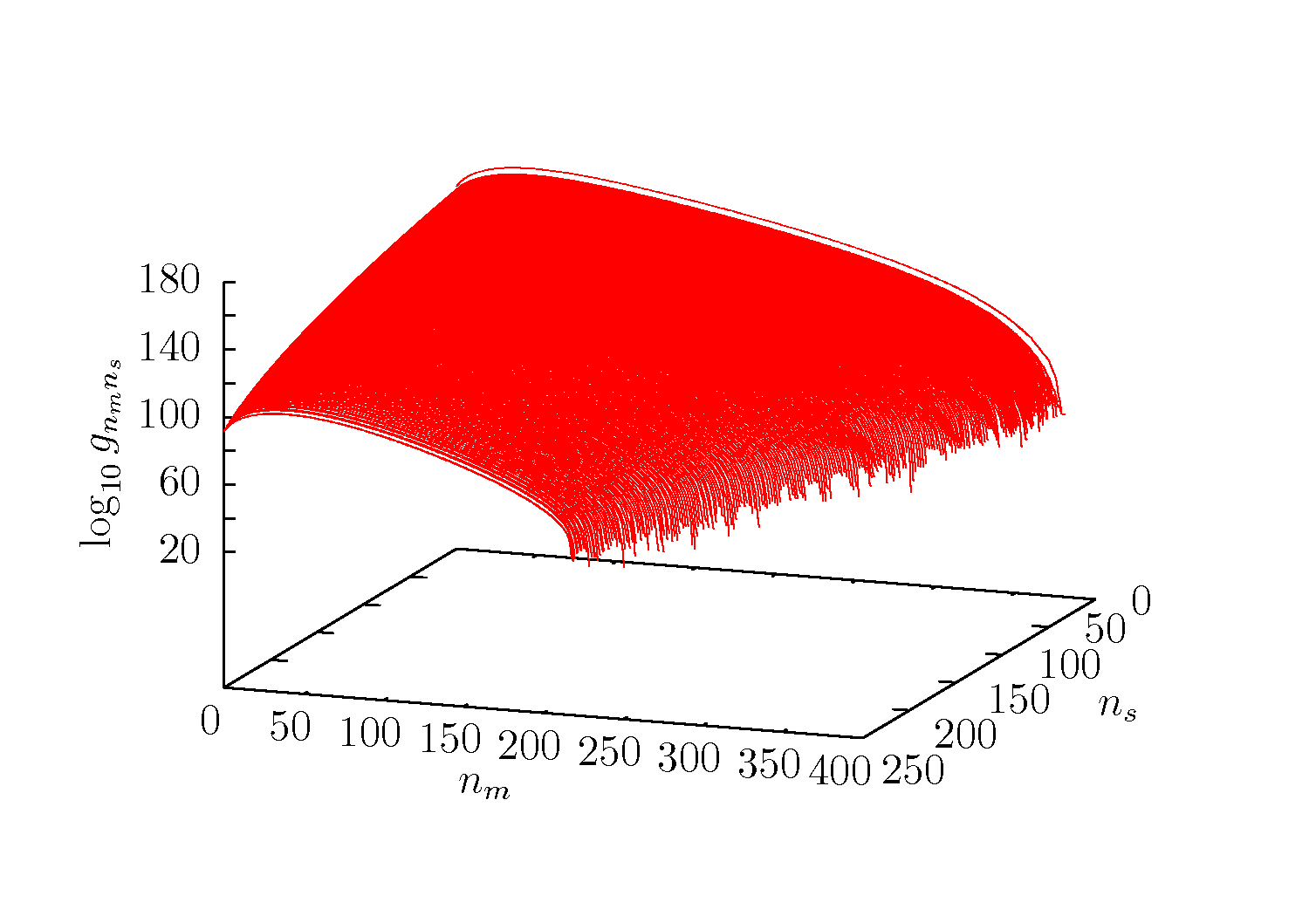
Figure 1: Contact density as a function of the number of monomer–monomer contacts $n_{m}$ and monomer–substrate contacts $n_{s}$ for a 250mer interacting with a solid substrate.

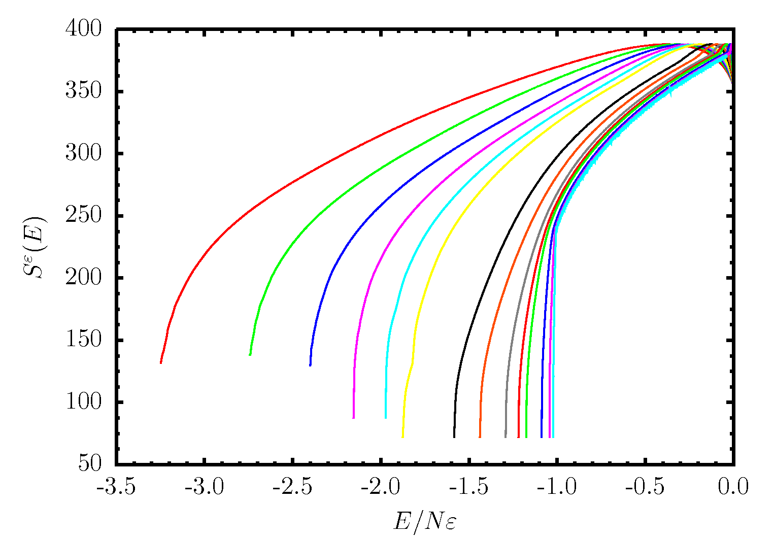
Figure 2: Microcanonical entropies $S^{\varepsilon}(E)$ of the hybrid system, calculated from the contact density $g_{n_{m}n_{s}}$ for various surface attraction strengths: $\varepsilon=0.5,0.6,0.7,0.8,0.9,1.0,1.5,2.0,3.0,4.0,5.0,10.0,20.0,40.0$ (curves from left to right).

3 Microcanonical Entropy in Dependence of the Surface Attraction Strength

The advantage of having estimated the contact density becomes obvious if we are interested in the transition behavior of the hybrid polymer–substrate system for different parametrizations of energy scales in the model (1). Since the microcanonical entropies can easily be calculated from the contact density,

$$S^{\varepsilon}(E)=k_{B}\ln\sum\limits_{n_{m},n_{s}}\delta_{E,E^{\varepsilon}_{n_{m}n_{s}}}g_{n_{m}n_{s}},$$ (2)

where $\delta_{ij}$ is the Kronecker symbol ($1$ if $i=j$, $0$ otherwise), the qualitative differences between the different models are apparent when comparing $S^{\varepsilon}(E)$ for various interaction strengths $\varepsilon$. Several exemplified entropy curves are shown in Fig. 2 for numerous values of $\varepsilon$ between $0.5$ and $40.0$ ($k_{B}=1$). Note once more that no additional simulations were required to obtain these substantially different results. The first interesting observation is that for $\varepsilon<1.0$, the ground-state entropies are larger than for models with $\varepsilon\geq 1.0$. The reason is that in the latter case the ground-state conformations are filmlike (topologically two-dimensional). In this case, it is more favorable for the system to maximize the number of surface contacts, even at the expense of the reduction of monomer–monomer contacts. The ground-state entropy is virtually constant and since the ground-state energy $E_{0}$ scales linearly with $\varepsilon$, $\lim_{\varepsilon\to\infty}E_{0}/N\varepsilon=-1$. The stepwisely increasing ground-state entropy for decreasing surface attraction strengths below $\varepsilon=1$ is due to layering effects (“dewetting”). For such model parametrizations, polymer ground-state conformations are topologically three-dimensional, i.e., they extend into the space direction perpendicular to the substrate [6]. Monomer–monomer contacts are energetically more favorable than surface contacts. The ground-state entropy increases, because the conformational entropy of a compact three-dimensional droplet is larger than for a compact film (the number of possible conformations is much larger in three dimensions).

The entropy curves also reveal all underlying informations regarding the conformational transitions such as, e.g., the adsorption transition. For small systems, it is a first-order-like transition characterized by phase coexistence. This can be investigated best by a microcanonical analysis [16, 17, 18]. In the high-energy regime, there is a convex region which causes a bimodal energy distribution at the transition temperature. Phases of adsorbed and desorbed are separated by a free–energy barrier which can be traced back to surface effects in the adsorption process. These effects disappear in the thermodynamic limit, where the adsorption transition is a continuous thermodynamic phase transition.

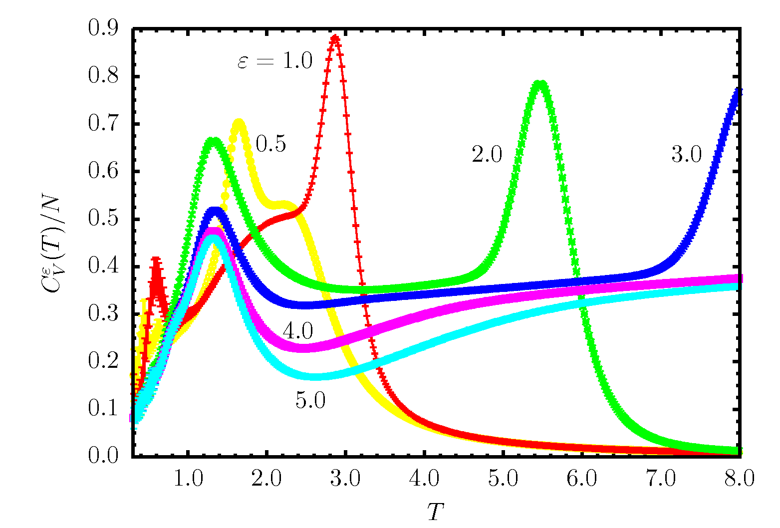
Figure 3: Specific heat as a function of temperature for various values of $\varepsilon$.

From the density of states $g^{\varepsilon}(E)=\exp[S^{\varepsilon}(E)/k_{B}]$, the canonical expectation value of the energy is calculated as

$$\langle E\rangle^{\varepsilon}=\frac{\sum_{E}Eg^{\varepsilon}(E)e^{-E/k_{B}T}}{\sum_{E}g^{\varepsilon}(E)e^{-E/k_{B}T}},$$ (3)

where $T$ is the heatbath temperature. The derivative of the mean energy defines the heat capacity: $C^{\varepsilon}_{V}(T)=d\langle E\rangle^{\varepsilon}/dT$. This quantity is shown in Fig. 3 for a number of $\varepsilon$ parameter values. Although canonical averages tend to smear out relevant statistical informations for small systems, the peak structure of the specific heat can give some insights into the transition behavior. For $\varepsilon\geq 1.0$, the pronounced high-temperature peaks indicate the adsorption/desorption transition. Peaks and shoulders below these transition temperatures belong to structure formation processes on the substrate (such as the collapse from expanded conformations to very compact, filmlike structures near $T=1.2$ for $\varepsilon\geq 2.0$). An exception is the curve for $\varepsilon=0.5$ which exhibits a shoulder above the adsorption transitions near $T=2.3$ which signals the collapse transition in the desorption regime (i.e., the well-known $\Theta$ collapse in solvent).

To conclude, we have shown that the contact density is a particularly helpful quantity for understanding structural transitions accompanying the adsorption behavior of a flexible lattice polymer. Derived from it, microcanonical and canonical quantities enable the quantitative analysis of the transitions and allow for the identification of transition points.

This work is partially supported by the Umbrella program under Grant No. SIM6. Supercomputer time of the Forschungszentrum Jülich under Project Nos. jiff39 and jiff43 is acknowledged.

References

- [1] M. Bachmann and W. Janke, Lect. Notes Phys. 736, 203 (2008).
- [2] E. Eisenriegler, K. Kremer, and K. Binder, J. Chem. Phys. 77, 6296 (1982).
- [3] E. Eisenriegler, Polymers near Surfaces: Conformation Properties and Relation to Critical Phenomena (World Scientific, Singapore, 1993).
- [4] T. Vrbová and S. G. Whittington, J. Phys. A 29, 6253 (1996); J. Phys. A 31, 3989 (1998); T. Vrbová and K. Procházka, J. Phys. A 32, 5469 (1999).
- [5] Y. Singh, D. Giri, and S. Kumar, J. Phys. A 34, L67 (2001); R. Rajesh, D. Dhar, D. Giri, S. Kumar, and Y. Singh, Phys. Rev. E 65, 056124 (2002).
- [6] M. Bachmann and W. Janke, Phys. Rev. Lett. 95, 058102 (2005); Phys. Rev. E 73, 041802 (2006); Phys. Rev. E 73, 020901(R) (2006).
- [7] J. Krawczyk, T. Prellberg, A. L. Owczarek, and A. Rechnitzer, Europhys. Lett. 70, 726 (2005).
- [8] J. Luettmer-Strathmann, F. Rampf, W. Paul, and K. Binder, J. Chem. Phys. 128, 064903 (2008).
- [9] M. Möddel, M. Bachmann, and W. Janke, J. Phys. Chem. B 113, 3314 (2009).
- [10] B. A. Berg and T. Neuhaus, Phys. Lett. B 267, 249 (1991); Phys. Rev. Lett. 68, 9 (1992).
- [11] M. Bachmann and W. Janke, Phys. Rev. Lett. 91, 208105 (2003); J. Chem. Phys. 120, 6779 (2004).
- [12] T. Prellberg and J. Krawczyk, Phys. Rev. Lett. 92, 120602 (2004).
- [13] M. N. Rosenbluth and A. W. Rosenbluth, J. Chem. Phys. 23, 356 (1955).
- [14] P. Grassberger, Phys. Rev. E 56, 3682 (1997).
- [15] H.-P. Hsu, V. Mehra, W. Nadler, and P. Grassberger, J. Chem. Phys. 118, 444 (2003); Phys. Rev. E 68, 21113 (2003).
- [16] D. H. E. Gross, Microcanonical Thermodynamics (World Scientific, Singapore, 2001).
- [17] C. Junghans, M. Bachmann, and W. Janke, Phys. Rev. Lett. 97, 218103 (2006); J. Chem. Phys. 128, 085103 (2008); Europhys. Lett. 87, 40002 (2009).
- [18] M. Möddel, W. Janke, and M. Bachmann, PhysChemChemPhys, in press (2010).