Cavity-free Photon Blockade Induced by Many-body Bound States

Abstract

The manipulation of individual, mobile quanta is a key goal of quantum communication; to achieve this, nonlinear phenomena in open systems can play a critical role. We show theoretically that a variety of strong quantum nonlinear phenomena occur in a completely open one-dimensional waveguide coupled to an $N$-type four-level system. We focus on photon blockade and the creation of single photon states in the absence of a cavity. Many-body bound states appear due to the strong photon-photon correlation mediated by the four-level system. These bound states cause photon blockade, which can generate a sub-Poissonian single-photon source.

The exchange and control of mobile qubits of information is a key part of both quantum communication and quantum information processing. A “quantum network” is an emerging paradigm Kimble (2008); Duan and Monroe (2010) combining these two areas: local quantum nodes of computing or end-users linked together by conduits of flying qubits. The determinisitic approach to the interaction between the local nodes and the conduits relies on cavities to provide the necessary strong coupling. Indeed, strong coupling between light and matter has been demonstrated using cavities in both the classic cavity quantum electrodynamics (QED) systems Mabuchi and Doherty (2002) and the more recent circuit-QED implementations Schoelkopf and Girvin (2008). This has enabled the observation of nonlinear optical phenomena at the single photon level, such as electromagnetically induced transparency (EIT) Mücke et al. (2010); Abdumalikov et al. (2010) and photon blockade Birnbaum et al. (2005); Lang et al. (2011). Experiments have also demonstrated the efficient exchange of information between a stationary qubit (atom) and flying qubits (photons) Boozer et al. (2007); Hofheinz et al. (2009). However, scaling cavity systems to a multi-node quantum network is still challenging because of the difficulty of connecting cavities and managing losses.

A new scheme for achieving strong coupling between light and atoms (or artificial atoms) has been recently proposed based on one-dimensional (1D) waveguides Chang et al. (2006); Shen and Fan (2007a); Chang et al. (2007); Zheng et al. (2010); Roy (2011); Kolchin et al. (2011), dubbed “waveguide QED” Zheng et al. (2010); Kolchin et al. (2011). Tremendous experimental progress in achieving strong coupling has occurred in a wide variety of such systems: a metallic nanowire coupled to a quantum dot Akimov et al. (2007), a diamond nanowire coupled to a nitrogen-vacancy center Babinec et al. (2010), a photonic nanowire with an embedded quantum dot Claudon et al. (2010), and a 1D superconducting transmission line coupled to a flux qubit Astafiev et al. (2010). In these systems, “strong coupling” means that the majority of the spontaneously emitted light is guided into waveguide modes; it is achieved through the tight confinement of optical fields in the transverse direction. Furthermore, waveguide systems are naturally scalable for quantum networking Kimble (2008). The key physical element introduced by the waveguide QED geometry is that the atom couples to a continuum of modes. This relaxes the restriction of working with a narrow cavity bandwidth; more importantly, interaction with a continuum brings in novel many-body effects that have no analogue in a cavity.

In this work, we show that the nonlinear optical phenomena EIT, photon blockade, and photon-induced tunneling emerge in a waveguide system for parameters Astafiev et al. (2010) that are currently accessible. For these dramatic and potentially useful nonlinear effects, it is necessary to consider a four-level system (4LS) rather than simply a two- or three-level system. Photon blockade and photon-induced tunneling have a completely different origin here from the cavity case Birnbaum et al. (2005); Faraon et al. (2008): they are produced by many-body bound states Shen and Fan (2007a); Zheng et al. (2010); Roy (2011); Nishino et al. (2009), whose amplitude decays exponentially as a function of the relative coordinates of the photons. Such states do not exist in cavities because a continuum of modes in momentum space is needed for the formation of bound-states in real space. We demonstrate the capability of such a system to generate a single-photon source, which is crucial for quantum cryptography and distributed quantum networking. Our work thus opens a new avenue toward the coherent control of light at the single-photon level based on a cavity-free scheme.

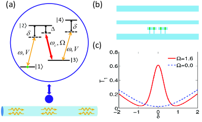
Figure 1: Schematic diagram of the waveguide system and EIT. (a) $N$-type four-level system interacting with the waveguide continuum. The transitions $|1\rangle\leftrightarrow|2\rangle$ and $|3\rangle\leftrightarrow|4\rangle$ are coupled to the waveguide modes with strength $V$, detuning $\delta$. The transition $|2\rangle\leftrightarrow|3\rangle$ is driven by a semiclassical control field with Rabi frequency $\Omega$ and detuning $\Delta$. Here, $\omega$ and $\omega_{c}$ are the frequencies of the incoming photons and the control field. (b) Schematic of possible experimental setup based on superconducting charge qubits Rebić et al. (2009). Two charge qubits, each formed from two Josephson junctions [dark gray (green) regions], are coupled capacitively to each other and to a transmission line (1D waveguide). (c) Single-photon transmission probability as a function of incident photon detuning. EIT occurs when the control field is on ($\Omega=1.6$, solid); when it is off, the 4LS becomes a two-level system and EIT disappears. Here, the effective Purcell factor is $P=6$.

Motivated by recent experimental advances Astafiev et al. (2010), we consider an $N$-type 4LS Majer et al. (2010); Rebić et al. (2009) coupled to a continuum of modes in a 1D waveguide. Figure 1 shows both a schematic and a possible realization using superconducting circuits Rebić et al. (2009). The Hamiltonian of the system is Shen and Fan (2007a); Zheng et al. (2010)

$$H=\int\!\!dx\,(-i)\hbar c\Big{[}a_{R}^{\dagger}(x)\frac{d}{dx}a_{R}(x)-a_{L}^{\dagger}(x)\frac{d}{dx}a_{L}(x)\Big{]}$$ (1)

$$+ \!\int\!\!dx\,\hbar V\delta(x)\big{\{}[a_{R}^{\dagger}(x)+a_{L}^{\dagger}(x)]\big{(}|1\rangle\langle 2|+|3\rangle\langle 4|\big{)}+{\rm h.c.}\big{\}},$$

$$+ \sum_{j=2}^{4}\hbar\Big{(}\epsilon_{j}-\frac{i\Gamma_{j}}{2}\Big{)}|j\rangle\langle j|+\frac{\hbar\Omega}{2}\Big{(}|2\rangle\langle 3|+{\rm h.c.}\Big{)},$$

where $a_{L,R}^{\dagger}(x)$ are the creation operators for left,right-going photons at position $x$ and $c$ is the group velocity of photons. In the 4LS, the energy reference is the energy of state $|1\rangle$ (the ground state), and $\epsilon_{2}=\omega_{21}$, $\epsilon_{3}=\epsilon_{2}-\Delta$, and $\epsilon_{4}=\epsilon_{3}+\omega_{43}$, where $\omega_{21}$ and $\omega_{43}$ are the $|1\rangle\leftrightarrow|2\rangle$ and $|3\rangle\leftrightarrow|4\rangle$ transition frequencies, respectively. In the spirit of the quantum jump picture Carmichael (1993), an imaginary term is included in the 4LS to model the spontaneous emission of the excited states at rate $\Gamma_{j}$ to modes other than the 1D waveguide continuum. We have assumed a linear dispersion and a frequency-independent coupling strength $V$ for the relevant frequency range Chang et al. (2007). The decay rate into the waveguide modes is $\Gamma\equiv 2V^{2}/c$ from Fermi’s golden rule. Below, we assume that level $|3\rangle$ is metastable ($\Gamma_{3}=0$) and levels $|2\rangle$ and $|4\rangle$ have the same loss rate ($\Gamma_{2}=\Gamma_{4}$).

A figure of merit to characterize the coupling strength is given by the effective Purcell factor, $P=\Gamma/\Gamma_{2}$. In an experiment with surface plasmons coupled to a quantum dot Akimov et al. (2007), $P=1.5$ was achieved. In more recent experiments, even larger Purcell factors, $P=3$ and $P\geq 9$, were demonstrated with a superconducting transmission line Astafiev et al. (2010) and a GaAs photonic nanowire Claudon et al. (2010); Bleuse et al. (2011), respectively. These recent dramatic experimental achievements suggest that the large Purcell-factor physics, which we now discuss, is presently within reach experimentally.

To study interaction effects during photon transmission, we obtain an exact solution of the scattering problem defined by Eq. (1). The scattering eigenstates are obtained by imposing an open boundary condition and requiring that the incident photon state be a free plane wave, an approach adopted previously to solve an interacting resonant-level model Nishino et al. (2009) and a two-level system problem Zheng et al. (2010). For an incident photon from the left (with wave-vector $k$) and the 4LS initially in its ground state, the transmitted part of the single-photon eigenstate is

$$\phi_{R}(x)=t_{k}e^{ikx}$$ (2)

$$t_{k}=\frac{[ck-\epsilon_{2}+\Delta+\frac{i\Gamma_{3}}{2}][ck-\epsilon_{2}+\frac{i\Gamma_{2}}{2}]-\frac{\Omega^{2}}{4}}{[ck-\epsilon_{2}+\Delta+\frac{i\Gamma_{3}}{2}][ck-\epsilon_{2}+\frac{i\Gamma_{2}}{2}+\frac{i\Gamma}{2}]-\frac{\Omega^{2}}{4}},\quad$$

where $t_{k}$ is the transmission coefficient. In the two-photon scattering eigenstate, the transmitted wave is

$$\phi_{RR}(x_{1},x_{2}) = t_{k_{1}}t_{k_{2}}(e^{ik_{1}x_{1}+ik_{2}x_{2}}+e^{ik_{1}x_{2}+ik_{2}x_{1}})$$ (3)

$$+ b_{1}e^{-\gamma_{1}|x_{2}-x_{1}|}+b_{2}e^{-\gamma_{2}|x_{2}-x_{1}|},$$

where $b_{1,2}$ and $\gamma_{1,2}$ ($>0$) are functions of system parameters (see the Supplementary Information). The first term of $\phi_{RR}$ corresponds to transmission of the two photons as independent (identical) particles with the momentum of each photon conserved individually. The second term is a two-body bound state—note the exponential decay in the relative coordinate $|x_{2}-x_{1}|$—with two characteristic binding strengths $\gamma_{1}$ and $\gamma_{2}$. Such a state results from the nonlinear interaction between photons mediated by the 4LS. Physically, it originates from the momentum non-conserved processes of each individual photon (with conservation of total momentum). A similar bound state has been found in a 1D waveguide coupled to a two-level system Shen and Fan (2007a); Zheng et al. (2010), a $\Lambda$-type three-level system Roy (2011), as well as an open interacting resonant level model Nishino et al. (2009).

We evaluate the transmission and reflection probabilities using the S-matrices constructed from the exact scattering eigenstates Zheng et al. (2010). Because any state containing a finite number of photons is, in practice, a wave packet, we consider a continuous mode input state Loudon (2003), whose spectrum is Gaussian with central frequency $\omega_{0}$ and width $\sigma$. Throughout this paper, we set the loss rate as the reference unit for all other quantities: $\Gamma_{2}=\Gamma_{4}=1$. The Purcell factor becomes $P=\Gamma/\Gamma_{2}=\Gamma$. For all the numerical results shown, we take the detuning of the control field to be zero, $\Delta=0$, and choose $\sigma=\Gamma_{2}/5=0.2$. In addition, we assume that the transitions $|1\rangle\leftrightarrow|2\rangle$ and $|3\rangle\leftrightarrow|4\rangle$ are at the same frequency ($\omega_{21}=\omega_{43}$).

Figure 1(c) shows that the transmission probability $T_{1}$ of a single photon has a sharp peak as a function of its detuning $\delta\equiv\omega_{0}-\omega_{21}$, demonstrating the familiar EIT phenomenon Witthaut and Sørensen (2010); Roy (2011) produced by interference between two scattering pathways. The width of the EIT peak is $\sim\!\Omega$ for $P\gg 1$ and is mainly determined by the control field strength $\Omega$. Here, we use $P=6$, a conservative value given the recent advances in experiments Claudon et al. (2010); Astafiev et al. (2010); Bleuse et al. (2011). When the control field is turned off, the 4LS becomes a two-level system, which acts as a reflective mirror Chang et al. (2007).

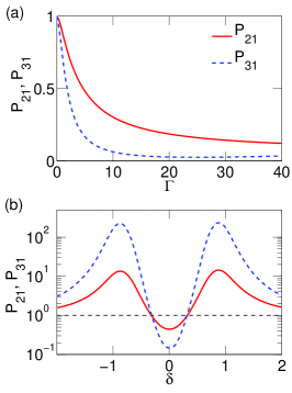
Figure 2: Photon blockade in transmission. (a) Photon blockade strength $P_{21}$ (solid) and $P_{31}$ (dashed) as a function of the decay rate $\Gamma$ into the waveguide modes (photon blockade is strongest when $P_{21}$ is smallest). The photons are on resonance with the 4LS ($\delta=0$) and $\Omega=1.6$. Strong coupling produces substantial photon blockade despite EIT being present in the single photon properties. (b) $P_{21}$ and $P_{31}$ as a function of the incident photon detuning $\delta$ for $\Gamma=6$ and $\Omega=1.6$. There is clear photon blockade on resonance as well as photon-induced tunneling ($P_{21},P_{31}>1$) on the sides of the resonance.

The EIT picture changes dramatically when there are two or more photons injected into the system. The 4LS mediates an effective photon-photon interaction, which in turn affects the multi-photon transmission. We define $T_{2}$ ($T_{3}$) to be the two- (three-) photon transmission probability of the two- (three-) photon scattering process. The strength of the photon blockade $P_{21}$ is given by the conditional probability $T_{2}/T_{1}$ for transmitting a second photon given that the first photon has already been transmitted, normalized by the single-photon transmission probability $T_{1}$: $P_{21}\equiv T_{2}/T_{1}^{2}$. For independent photons, there is no photon blockade and $P_{21}=1$. In the opposite limit of strong photon blockade, $P_{21}$ is suppressed towards zero. Similarly, we define $P_{31}\equiv T_{3}/T_{1}^{3}$ to quantify photon blockade in the three photon case.

A pronounced photon blockade is shown in Fig. 2(a) in the strong coupling regime: the single photon EIT effect does not carry over to the multi-photon case. For increasing coupling strength, both $P_{21}$ and $P_{31}$ approach zero. Such photon blockade regulates the flow of photons in an ordered manner, enabling coherent control over the information transfer process in our cavity-free scheme. Taking $P=9$ achieved in Ref. Claudon et al., 2010, we obtain the values $P_{21}\sim 30\%$ and $P_{31}\sim 7\%$, showing that the effects predicted here are already within reach of experiments.

The photon blockade occurs despite being in the EIT regime: as shown in Fig. 2(b), both $P_{21}$ and $P_{31}$ are suppressed within the EIT window, whose width is set by the control field strength $\Omega$. However, away from the EIT window, $P_{21}$ and $P_{31}$ become larger than $1$, signaling a new regime of multi-photon transmission—photon-induced tunneling Faraon et al. (2008). Previously, photon blockade and photon-induced tunneling have been observed in cavity-QED and circuit-QED systems Birnbaum et al. (2005); Faraon et al. (2008); Lang et al. (2011), where the underlying mechanism is the anharmonicity of the spectrum caused by the atom-cavity coupling. We emphasize that such anharmonicity is absent in the present cavity-free scheme: the photon blockade and photon-induced tunneling here must be caused by a different mechanism.

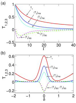
Figure 3: Many-body bound-state effect causing photon blockade. (a) Transmission as a function of the decay rate $\Gamma$ into the waveguide modes for $\Omega=1.6$. The presence of the many-body bound states suppresses the multi-photon transmission. (b) Transmission as a function of incident photon detuning $\delta$ for $\Gamma=6$ and $\Omega=1.6$. The bound states strikingly oppose multi-photon EIT; off-resonance, their constructive interference produces photon-induced tunneling.

To understand the origin of these phenomena, we separate the two-photon transmission probability $T_{2}$ into two parts (Fig. 3): $(T_{2})_{\rm PW}=T_{1}^{2}$ is the contribution from independent transmission and $(T_{2})_{\rm BS}$ is the contribution from both the bound-state term in Eq. (3) and the interference between the plane-wave and bound-state terms. $(T_{2})_{\rm BS}$ is the result of the many-body interactions in the waveguide and is absent for cavities. Similarly, $T_{3}$ can be separated into $(T_{3})_{\rm PW}=T_{1}^{3}$ and $(T_{3})_{\rm BS}$. Figure 3(a) shows that, when the photons are on resonance, $(T_{2,3})_{\rm BS}$ is always negative, suppressing the overall transmission. The cause of the observed photon blockade is, thus, the destructive interference between the two transmission pathways: passing by the 4LS as independent particles or as a composite particle in the form of bound states. Within the EIT window, this conclusion always holds (see Fig. 3(b))—both two- and three-photon transmission are strongly suppressed by the many-body bound-state effect. In contrast, away from the EIT window, $(T_{2,3})_{\rm BS}$ changes sign and becomes positive (see the Supplementary Information for a detailed analysis of the interference). Destructive interference changes to constructive interference, producing photon-induced tunneling.

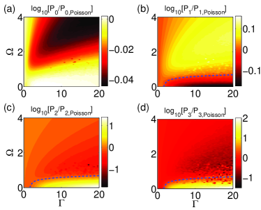
Figure 4: Non-classical photon states. Photon number statistics quantified by $\text{log}_{10}(P_{n}/P_{n,\text{Poisson}})$, where the probability of $n$ photons in the output state is $P_{n}$ and $P_{n,\text{Poisson}}$ is for a coherent state with the same mean photon number. Panels (a)-(d) show results for $n=0,1,2,$ and $3$, respectively, as a function of the control field strength $\Omega$ and the decay rate $\Gamma$. The dashed line is a guide to the eye indicating equal probabilities, $P_{n}/P_{n,\text{Poisson}}=1$. Note the large range of parameters for which the single photon probability is enhanced while the multi-photon content is suppressed—an improved single photon source.

As an application, we now show that the 4LS can generate non-classical photon states. We assume that the 4LS is in its ground state initially. We consider an incident continuous-mode coherent state of mean photon number $\bar{n}=1.0$, on resonance with the 4LS. The photon number statistics in the transmitted field can be obtained using the S-matrix method Zheng et al. (2010) and is presented in Fig. 4 by taking the ratio of the photon number distribution of the output state $P_{n}$ ($n=0,1,2,3$) to that of a coherent state $P_{n,\text{Poisson}}$ having the same mean photon number. It is remarkable that, in most of the parameter space, we have $P_{1}>P_{1,\text{Poisson}}$ while $P_{2}<P_{2,\text{Poisson}}$ and $P_{3}<P_{3,\text{Poisson}}$. This gives rise to a sub-Poissonian single-photon source: for example, for $\Gamma=9$ ($P=9$) and $\Omega=1.6$, we have $P_{0}=64\%$ and $P_{1}=34\%$ with the multi-photon probability $P_{n\geq 2}$ less than $3\%$, in comparison with $P_{n\geq 2}=26\%$ in the input. This single-photon source comes about because, under EIT conditions, a single photon passes through the system with high probability, while multi-photon states experience photon blockade caused by the bound-state effect. A systematic way of improving the quality of the single-photon source is to let a coherent state with a large mean photon number pass through multiple 4LS devices in series with Faraday isolators inserted between each stage.

In summary, we present a cavity-free scheme to realize a variety of nonlinear quantum optical phenomena—including EIT, photon blockade and photon-induced tunneling—in a 1D waveguide. Photon blockade and photon-induced tunneling have a distinctly different origin here compared to the cavity case: a many-body bound-state effect. Furthermore, we outline how to use EIT and photon blockade in this system to produce a single-photon source on demand. On the one hand, the demonstrated ability to control the flow of light quanta using EIT and photon blockade is a critical step towards the realization of an open quantum network. On the other hand, the strong photon-photon interaction mediated by the 4LS provides a new candidate system to study strongly correlated 1D systems, one complementary to condensed-matter systems.

The work of HUB and HZ was supported by the U.S. Office of Naval Research.

Supplementary Material for “Cavity-free Photon Blockade Induced by Many-body Bound States”

Hamiltonian

The Hamiltonian describing the interaction between a 1D continuum and a 4LS at the spatial origin is given by SM_ChangNatPhy07 ; SM_ShenPRA09 ,

$$H = \int dk\,\hbar\omega_{k}a^{\dagger}(k)a(k)+H_{4LS}+\int dk\,\hbar g\Big{\{}a^{\dagger}(k)\big{[}S_{12}+S_{34}\big{]}+h.c.\Big{\}},$$

$$H_{4LS} = \sum_{j=2}^{4}\hbar\left(\epsilon_{j}-\frac{i\Gamma_{j}}{2}\right)|j\rangle\langle j|+\frac{\hbar\Omega}{2}\left(|2\rangle\langle 3|+h.c.\right)$$ (S4)

where $g$ is the coupling strength, $S_{12}=|1\rangle\langle 2|$ and $S_{34}=|3\rangle\langle 4|$. Linearizing the dispersion around the transition energy of the 4LS and treating the left-going and right-going photons as separate fields, we obtain a two-mode Hamiltonian. Transformation to the real space field operators $a_{L(R)}(x)=(1/\sqrt{2\pi})\int dke^{ikx}a_{L(R)}(k)$ yields the real-space Hamiltonian

$$H=\int dx\hbar c[a_{R}^{\dagger}(x)(-i\frac{d}{dx})a_{R}(x)-a_{L}^{\dagger}(x)(-i\frac{d}{dx})a_{L}(x)]+H_{4LS}+\int dx\hbar V\Big{\{}[a_{R}^{\dagger}(x)+a_{L}^{\dagger}(x)]\big{[}S_{12}+S_{34}\big{]}+h.c.\Big{\}},$$ (S5)

where $V=\sqrt{2\pi}g$. Finally, the coupling between the 4LS and general modes other than the waveguide can be incorporated in the same manner as the waveguide-4LS interaction. Such interaction with general reservoir modes, such as vacuum modes, leads to intrinsic dissipation. This term can be treated by the Wigner-Weisskopf approximation SM_Meystre and so replaced by a non-Hermitian damping term in $H_{4LS}$ SM_ShenPRA09 ; SM_Carmichael93 , thus giving rise to the Hamiltonian in Eq. (1) of the main text.

Scattering Eigenstates

A key insight to solve for the scattering eigenstates is gained by performing the operator transformation

$$a_{e/o}^{\dagger}(x)\equiv\big{[}a_{R}^{\dagger}(x)\pm a_{L}^{\dagger}(-x)\big{]}/\sqrt{2}.$$ (S6)

The Hamiltonian is then decomposed into even and odd modes: $H=H_{e}+H_{o}$ with

$$H_{e} = \int dx(-i)\hbar c\hat{a}_{e}^{\dagger}(x)\frac{d}{dx}\hat{a}_{e}(x)+H_{4LS}$$ (S7)

$$+\int dx\,\hbar\sqrt{2}V\,\delta(x)\big{[}\hat{a}_{e}^{\dagger}(x)(S_{12}+S_{34})+h.c.\big{]},$$

$$H_{o} = \int dx(-i)\hbar c\hat{a}_{o}^{\dagger}(x)\frac{d}{dx}\hat{a}_{o}(x).$$

Because $[H,\hat{n}_{e}+\hat{n}_{{\rm 4LS}}]=[H,\hat{n}_{o}]=0$ for the number operators $\hat{n}_{e/o}\equiv\int dx\hat{a}_{e/o}^{\dagger}(x)\hat{a}_{e/o}(x)$ and $\hat{n}_{{\rm 4LS}}\equiv\sum_{j=2,3}|j\rangle\langle j|+2|4\rangle\langle 4|$, the total number of excitations in both the even and odd spaces are separately conserved. We will now focus on finding the non-trivial even-mode solution and then transform back to the left/right representation. A general $n$-excitation state ($n=n_{e}+n_{{\rm 4LS}}$) in the even space is given by

$$|\Psi_{n}\left\rangle\right. = \bigg{(}\int dx^{n}\,g^{(n)}(x)\,\hat{a}_{e}^{\dagger}(x_{1})\cdots\hat{a}_{e}^{\dagger}(x_{n})$$ (S8)

$$+ \int dx^{n-1}\,\big{[}f_{2}^{(n)}(x)S_{12}^{+}+f_{3}^{(n)}(x)S_{13}^{+}\big{]}\ \hat{a}_{e}^{\dagger}(x_{1})\cdots\hat{a}_{e}^{\dagger}(x_{n-1}),$$

$$+ \int dx^{n-2}\,f_{4}^{(n)}(x)S_{14}^{+}\hat{a}_{e}^{\dagger}(x_{1})\cdots\hat{a}_{e}^{\dagger}(x_{n-2})\bigg{)}|0,1\rangle$$

where $|0,1\rangle$ is the zero photon state with the 4LS in the ground state $|1\rangle$.

The scattering eigenstates are constructed by imposing the boundary condition that, in the incident region $x_{1},\cdots,x_{n}<0$, $g^{(n)}(x_{1},\cdots,x_{n})$ is a free plane wave SM_NishinoPRL09 ; SM_ZhengPRA10 . The one-photon scattering eigenstate with eigenenergy $E=ck$ is given by

$$g^{(1)}(x) = g_{k}(x)=h_{k}(x)[\theta(-x)+\bar{t}_{k}\theta(x)],\,\,\,\,\,\,\,\,\,\,\,\,\,\,\,\,h_{k}(x)\equiv\frac{e^{ikx}}{\sqrt{2\pi}},\,\,\,$$

$$f_{2}^{(1)} = \frac{ic}{\sqrt{2\pi\Gamma}}(\bar{t}_{k}-1),$$ (S9)

$$f_{3}^{(1)} = \frac{ic\Omega}{\sqrt{8\pi\Gamma}}\frac{(\bar{t}_{k}-1)}{ck+\Delta+i\Gamma_{3}/2-\epsilon_{2}},$$

$$\bar{t}_{k} = \frac{[ck-\epsilon_{2}+\Delta+i\Gamma_{3}/2][ck-\epsilon_{2}+i\Gamma_{2}/2-i\Gamma/2]-\Omega^{2}/4}{[ck-\epsilon_{2}+\Delta+i\Gamma_{3}/2][ck-\epsilon_{2}+i\Gamma_{2}/2+i\Gamma/2]-\Omega^{2}/4},$$

where $\theta(x)$ is the step function and $\Gamma=2V^{2}/c$ is the spontaneous emission rate to the 1D continuum. Notice that the amplitude $f_{4}^{(1)}$ vanishes because it takes two excitation quanta to excite level $|4\rangle$. Therefore, for one-photon scattering, the 4LS behaves as a three-level system and Eq. (S9) coincides with previous studies SM_WitthautNJP10 ; SM_RoyPRL11 . Transforming from the even/odd back to the left/right representation gives rise to the wavefunction of one photon transmission in the single-photon scattering, shown in Eq. (2) in the main text, where $t_{k}=(\bar{t}_{k}+1)/2$.

For two-photon scattering, starting from a free plane wave in the region $x_{1},x_{2}<0$, we use the Schrodinger equation implied by $H_{e}$ in Eq. (S7) to find the wave function first in the region $x_{1}<0<x_{2}$ and then for $0<x_{1},x_{2}$. The method is explained in detail in the appendix of Ref. SM_ZhengPRA10 for scattering from a two level system. We obtain the two-photon scattering eigenstate with eigenenergy $E=ck_{1}+ck_{2}$

$$g^{(2)}(x_{1},x_{2}) = \frac{1}{2}\sum_{Q}\left[g_{k_{1}}(x_{Q_{1}})g_{k_{2}}(x_{Q_{2}})+B(x_{Q_{1}},x_{Q_{2}})\right],$$

$$f_{2}^{(2)}(x) = \sum_{Q}\frac{ic(\bar{t}_{k_{Q_{1}}}-1)g_{k_{Q_{2}}}(x)}{\sqrt{2\pi\Gamma}}+\frac{ice^{iEx}}{\sqrt{\Gamma}}[C_{1}e^{\lambda_{1}x}+C_{2}e^{\lambda_{2}x}]\theta(x),$$

$$f_{3}^{(3)}(x) = \frac{c\Omega\sqrt{\Gamma}}{\sqrt{8\pi}}\sum_{Q}\frac{g_{k_{Q_{1}}}(x)}{\rho_{k_{Q_{2}}}}-\frac{2ce^{iEx}}{\sqrt{\Gamma}\Omega}[\kappa_{1}C_{1}e^{\lambda_{1}x}+\kappa_{2}C_{2}e^{\lambda_{2}x}]\theta(x),$$

$$f_{4}^{(2)} = \sum_{Q}\frac{ic\Omega(\bar{t}_{k_{Q_{1}}}-1)}{4\pi\rho_{k_{Q_{2}}}}-\frac{2ic\beta}{\Gamma\Omega},$$ (S10)

$$B(x_{Q_{1}},x_{Q_{2}}) = e^{iEx_{Q_{2}}}[C_{1}e^{\lambda_{1}|x_{2}-x_{1}|}+C_{2}e^{\lambda_{2}|x_{2}-x_{1}|}]\theta(x_{Q_{2}}-x_{Q_{1}})\theta(x_{Q_{1}}),$$

where $Q=(Q_{1},Q_{2})$ is a permutation of $(1,2)$, and

$$c\lambda_{1} = -\frac{\Gamma+\Gamma_{2}+\Gamma_{3}}{4}+\xi+i(\frac{\Delta}{2}-\epsilon_{2}+\eta),\,\,\,\,\,\,\,\,\,\,\,\,\,c\lambda_{2}=-\frac{\Gamma+\Gamma_{2}+\Gamma_{3}}{4}-\xi+i(\frac{\Delta}{2}-\epsilon_{2}-\eta)$$

$$C_{1} = \frac{\beta-\alpha c\lambda_{2}}{\lambda_{1}-\lambda_{2}},\,\,\,\,\,\,\,\,\,\,\,\,\,C_{2}=-\frac{\beta-\alpha c\lambda_{1}}{\lambda_{1}-\lambda_{2}},$$

$$\rho_{k} = \left(ck-\epsilon_{2}+\Delta+\frac{i\Gamma_{3}}{2}\right)\left(ck-\epsilon_{2}+\frac{i\Gamma_{2}+i\Gamma}{2}\right)-\frac{\Omega^{2}}{4},\,\,\,\,\,\,\,\,\,\,\,\,\,\chi=\Delta^{2}+\Omega^{2}-\Gamma^{\prime 2}$$

$$\kappa_{1} = \frac{\Gamma^{\prime}}{2}+\xi+i(\frac{\Delta}{2}+\eta),\,\,\,\,\,\,\,\,\,\,\,\,\,\,\,\,\,\,\,\,\,\,\,\,\,\,\,\kappa_{2}=\frac{\Gamma^{\prime}}{2}-\xi+i(\frac{\Delta}{2}-\eta),$$

$$\xi = \frac{\sqrt{2}}{4}\sqrt{\sqrt{\chi^{2}+4\Delta^{2}\Gamma^{\prime 2}}-\chi},\,\,\,\,\,\,\,\,\,\,\,\,\,\eta=\frac{\sqrt{2}}{4}\sqrt{\sqrt{\chi^{2}+4\Delta^{2}\Gamma^{\prime 2}}+\chi}$$

$$\alpha = -\frac{(\bar{t}_{k_{1}}-1)(\bar{t}_{k_{2}}-1)}{\pi},\,\,\,\,\,\,\,\,\,\,\,\,\,\,\,\,\,\,\,\,\,\,\,\,\,\,\,\beta=\frac{-\Gamma\Omega^{2}}{8\pi}\left[\frac{\nu-\bar{t}_{k_{1}}}{\rho_{k_{2}}}+\frac{\nu-\bar{t}_{k_{2}}}{\rho_{k_{1}}}\right],$$

$$\Gamma^{\prime} = \frac{\Gamma+\Gamma_{2}-\Gamma_{3}}{2},\,\,\,\,\,\,\,\,\,\,\,\,\,\,\,\,\,\,\,\,\,\,\,\,\,\,\,\,\,\,\,\,\,\,\,\,\,\,\,\,\,\,\,\,\,\,\nu=\frac{\epsilon_{4}-E-(i\Gamma_{4}-i\Gamma)/2}{\epsilon_{4}-E-(i\Gamma_{4}+i\Gamma)/2}.$$ (S11)

Again, performing an even/odd to left/right transformation SM_ZhengPRA10 , we obtain the wavefunction of two photon transmission in two-photon scattering, shown in Eq. (3) in the main text. There, $\gamma_{1/2}=-\text{Re}[\lambda_{1/2}]$ and $b_{1/2}\propto C_{1/2}$. In the case that $\Delta=\Gamma_{3}=0$, $\xi=|\chi|\theta(-\chi)/2$ and $\eta=|\chi|\theta(\chi)/2$ with $\chi=\Omega^{2}-\left(\Gamma+\Gamma_{2}\right)^{2}/4$, where again $\theta(x)$ is the step function.

From the scattering eigenstates, scattering matrices can be constructed using the Lippmann-Schwinger formalism SM_Sakurai . The output states are then obtained by applying the scattering matrices on the incident photon states (single-, two-, and three-photon number states as well as coherent states). By performing measurement operations on the output states, we obtain the transmission and reflection probabilities and photon number statistics. A general procedure is outlined in Ref. SM_ZhengPRA10 .

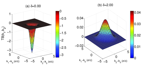
Figure 5: The integrand function $TB(k_{1},k_{2})$ of the interference term as a function of $k_{1}$and $k_{2}$. (a) $\delta=0.0$. (b) $\delta=2.0$.

Phase Analysis of Photon Blockade and Photon-Induced Tunneling

In Fig. 3 of the main text, we show that the observed photon blockade and photon-induced tunneling orignate from destructive and constructive interference effects, respectively. In this section, we present a detailed analysis of the relative phase between the plane-wave and bound-state terms. The two-photon transmission probability $T_{2}$ for the two-photon scattering is given by

$$T_{2}=\int dk_{1}dk_{2}|T(k_{1},k_{2})+B(k_{1},k_{2})|^{2},$$ (S12)

where $k_{1}$ and $k_{2}$ are the momenta of the two photons in the wavepacket. The plane-wave term $T(k_{1},k_{2})$ and the bound-state term $B(k_{1},k_{2})$ take the form

$$T(k_{1},k_{2}) = \alpha(k_{1})\alpha(k_{2})t_{k_{1}}t_{k_{2}}$$

$$B(k_{1},k_{2}) = \sum_{j=1,2}\frac{\sqrt{\Gamma}}{8}\left(\frac{1}{k_{1}-i\gamma_{j}}+\frac{1}{k_{2}-i\gamma_{j}}\right)\int dk^{\prime}\alpha(k^{\prime})\alpha(k_{1}+k_{2}-k^{\prime})C_{j}(k^{\prime},k_{1}+k_{2}-k^{\prime}),$$ (S13)

where $\alpha(k)$ is the amplitude of a Gaussian wavepacket with central frequency $\omega_{0}$ and width $\sigma$. In momentum space, the central momentum is $k_{0}=\omega_{0}/c$ and the width is $\sigma/c$, where $c$ is the group velocity of photons in the waveguide. By defining the phase difference $\theta(k_{1},k_{2})$ between $T(k_{1},k_{2})$ and $B(k_{1},k_{2})$, $T_{2}$ can be written as

$$T_{2}=\int dk_{1}dk_{2}|T(k_{1},k_{2})|^{2}+\int dk_{1}dk_{2}2|T(k_{1},k_{2})B(k_{1},k_{2})|\text{cos}\theta(k_{1},k_{2})+\int dk_{1}dk_{2}|B(k_{1},k_{2})|^{2},$$ (S14)

where the first term is the plane-wave term, the second term is the interference between the plane-wave and bound-state terms, and the third term is the contribution from the bound-state term. In the main text, the first term is denoted $(T_{2})_{PW}$ and the second and third terms together are called $(T_{2})_{BS}.$ Denote the intergrand function of the interference term as $TB(k_{1},k_{2})$,

$$TB(k_{1},k_{2})=2|T(k_{1},k_{2})B(k_{1},k_{2})|\text{cos}\theta(k_{1},k_{2})$$ (S15)

The phase $\theta(k_{1},k_{2})$, or specifically, the sign of $\text{cos}\theta(k_{1},k_{2})$, determines whether the interference is constructive or destructive.

We numerically evaluate $TB(k_{1},k_{2})$ in two cases: $\delta=\omega_{0}-\omega_{21}=0.0$ and $\delta=\omega_{0}-\omega_{21}=2.0$. Here, the unit of detuning $\delta$ is set by the loss rate $\Gamma_{2}$. All the other system parameters are the same as in Fig. 3b in the main text. Fig. 5 shows $TB(k_{1},k_{2})$ as a function of $k_{1}-k_{0}$ and $k_{2}-k_{0}$. As expected for a Gaussian packet, the value of $TB(k_{1},k_{2})$ is centered at $k_{1}=k_{2}=k_{0}$ in both cases. However, the sign of the peaks in the two cases differs. For $\delta=0.0$, a negative peak indicates destructive interference, giving rise to photon blockade when the incident photons are on resonane with the 4LS. For $\delta=2.0$, a positive peak indicates constructive interference, producing photon-induced tunneling when the photons are far off resonance.

References

- Kimble (2008) H. J. Kimble, Nature 453, 1023 (2008).
- Duan and Monroe (2010) L.-M. Duan and C. Monroe, Rev. Mod. Phys. 82, 1209 (2010).
- Mabuchi and Doherty (2002) H. Mabuchi and A. C. Doherty, Science 298, 1372 (2002).
- Schoelkopf and Girvin (2008) R. J. Schoelkopf and S. M. Girvin, Nature 451, 664 (2008).
- Mücke et al. (2010) M. Mücke et al., Nature 465, 755 (2010).
- Abdumalikov et al. (2010) A. A. Abdumalikov et al., Phys. Rev. Lett. 104, 193601 (2010).
- Birnbaum et al. (2005) K. M. Birnbaum et al., Nature 436, 87 (2005).
- Lang et al. (2011) C. Lang et al., Phys. Rev. Lett. 106, 243601 (2011).
- Boozer et al. (2007) A. D. Boozer et al., Phys. Rev. Lett. 98, 193601 (2007).
- Hofheinz et al. (2009) M. Hofheinz et al., Nature 459, 546 (2009).
- Chang et al. (2006) D. E. Chang, A. S. Sørensen, P. R. Hemmer, and M. D. Lukin, Phys. Rev. Lett. 97, 053002 (2006).
- Shen and Fan (2007a) J.-T. Shen and S. Fan, Phys. Rev. Lett. 98, 153003 (2007a); Phys. Rev. A 76, 062709 (2007b).
- Chang et al. (2007) D. E. Chang, A. S. Sørensen, E. A. Demler, and M. D. Lukin, Nature Phys. 3, 807 (2007).
- Zheng et al. (2010) H. Zheng, D. J. Gauthier, and H. U. Baranger, Phys. Rev. A 82, 063816 (2010).
- Roy (2011) D. Roy, Phys. Rev. Lett. 106, 053601 (2011).
- Kolchin et al. (2011) P. Kolchin, R. F. Oulton, and X. Zhang, Phys. Rev. Lett. 106, 113601 (2011).
- Akimov et al. (2007) A. V. Akimov et al., Nature 450, 402 (2007).
- Babinec et al. (2010) T. M. Babinec et al., Nature Nanotech. 5, 195 (2010).
- Claudon et al. (2010) J. Claudon et al., Nat. Photon. 4, 174 (2010).
- Astafiev et al. (2010) O. Astafiev et al., Science 327, 840 (2010).
- Faraon et al. (2008) A. Faraon et al., Nature Phys. 4, 859 (2008).
- Nishino et al. (2009) A. Nishino, T. Imamura, and N. Hatano, Phys. Rev. Lett. 102, 146803 (2009).
- Majer et al. (2010) J. B. Majer et al., Phys. Rev. Lett. 94, 090501 (2005).
- Rebić et al. (2009) S. Rebić, J. Twamley, and G. J. Milburn, Phys. Rev. Lett. 103, 150503 (2009).
- Carmichael (1993) H. J. Carmichael, An Open Systems Approach to Quantum Optics (Springer, Berlin, 1993).
- Bleuse et al. (2011) J. Bleuse et al., Phys. Rev. Lett. 106, 103601 (2011).
- Loudon (2003) R. Loudon, The Quantum Theory of Light (Oxford University Press, New York, 2003), 3rd ed.
- Witthaut and Sørensen (2010) D. Witthaut and A. S. Sørensen, New J. Phys. 12, 043052 (2010).

References

- (1) D. E. Chang, A. S. Sorensen, E. A. Demler, and M. D. Lukin, Nature Phys. 3, 807 (2007).
- (2) J. T. Shen, and S. Fan, Phys. Rev. A 79, 023837 (2009).
- (3) P. Meystre, and M. Sargent III, p. 351, Elements of Quantum Optics (Springer, New York, 1999), 3rd ed.
- (4) H. J. Carmichael, An Open Systems Approach to Quantum Optics (Lecture Notes in Physics) (Springer, Berlin, 1993).
- (5) A. Nishino, T. Imamura, and N. Hatano, Phys. Rev. Lett. 102, 146803 (2009).
- (6) H. Zheng, D. J. Gauthier, and H. U. Baranger, Phys. Rev. A 82, 063816 (2010).
- (7) D. Witthaut and A. S. Sorensen, New J. Phys. 12, 043052 (2010).
- (8) D. Roy, Phys. Rev. Lett. 106, 053601 (2011).
- (9) J. J. Sakurai, p. 379, Modern Quantum Mechanics (Addison-Wesley, Reading, MA, 1994).