0.33em 0.33em

Integrating out the heaviest quark in $N$–flavour $\chi$pt

Mikhail A. Ivanov¹ and Martin Schmid²

¹Bogoliubov Laboratory of Theoretical Physics, Joint Institute for Nuclear Research,
141980 Dubna, Russia

² Basler Versicherung AG, Aeschengraben 21,
4002 Basel, Switzerland

Abstract

We extend a known method to integrate out the strange quark in three flavour chiral perturbation theory to the context of an arbitrary number of flavours. As an application, we present the explicit formulæ to one–loop accuracy for the heavy quark mass dependency of the low energy constants after decreasing the number of flavours by one while integrating out the heaviest quark in $N$–flavour chiral perturbation theory.

Keywords: Chiral symmetries, Chiral perturbation theory, Chiral Lagrangian

pacs: 11.30.Rd, 12.39.Fe, 13.40.Dk, 13.40.Ks

1    Introduction

Chiral perturbation theory ($\chi$pt) [1, 2, 3] displays and exploits transparently the symmetries of low energy qcd. However, being an effective field theory, it also features a myriad of low–energy constants (lecs) that are not fixed by symmetry, but rather have to be determined from experiment. To aid this determination with additional constraints and gain some insight into the heavy quark mass dependence of these lecs, a series of publications[4, 5, 6, 7, 8, 9, 10, 11] has appeared in the recent past that presents relations among the lecs of different versions of $\chi$pt. This work will contribute to this line of publications, albeit in an unusual form, as it addresses a matching between the lecs of $\chi$pt with $N$ light quarks ($\chi$pt_N) and $\chi$pt_N-1, while the publications cited above concentrate on three– versus two–flavour physics. The reason for this generalisation lies in a possible interest of the lattice community in a matching between four– and three– flavour lecs. To not repeat ourselves with only different numbers, we chose to generalise the scope, as we do not know if there might arise some interest in other flavour combinations in the future.

The aim of this paper is to provide the dependence on the $N^{\text{th}}$ quark mass of the lecs of chiral perturbation theory of $N-1$ flavours to one–loop accuracy. This aim is achieved by the methods laid out in [12], namely calculating the generating functional for $\chi$pt_N in a limit where it describes only the physics of $\chi$pt_N-1. Comparing the coefficients of its local contributions with the action of $\chi$pt_N-1 yields the desired matching. This method is equivalent to evaluate and compare the Green’s functions of external fields of both theories, however, without the need for a cumbersome calculation and comparison of multiple matrix elements in both theories. The method can be used for higher loop calculations with only marginal complications (but at a significantly higher computational effort).

The publication is structured as follows: after this brief introduction, the formalism of $\chi$pt_N is laid out in Section 2 and in more detail in Appendix a. It follows a description of the technique used in Section 3. The technical details of the tree–level (Section b) and the loop calculations (Section c) are devoted their own space, summarised in Section 4. At the end, we add Section 5 with the results of the calculation, examples of application in Section 6 and a short summary in Section 7. In Appendix d, a reduction to the case $N=3$ is presented as a check of the calculations.

2    Preliminaries

In this section, we will shortly discuss the setup of $\chi$pt_N.

Chiral perturbation theory yields a consistent and systematic framework to explore the effects of symmetries in low energy qcd. The starting point is the massless qcd–Lagrangian $\mathcal{L}_{\sc qcd\rm{}}^{0}$, enriched with couplings to external (axial–) vector fields ($a_{\mu}$) $v_{\mu}$ and (pseudo–) scalar sources ($p$) $s$.

The leading order (Euclidean) Lagrangian reads

$$\mathcal{L}_{2}^{N}=\frac{F_{N}^{2}}{4}\langle u^{N}\cdot u^{N}-\chi^{N}_{+}\rangle\,,$$ (2.1)

where the above mentioned (axial–) vector fields are part of the building block $u_{\mu}^{N}$ and the (pseudo–) scalar fields are hidden in $\chi_{+}^{N}$. Consult Appendix a for the details of the notation. Visible is one of the two leading order lecs ($F_{N}$), while the other ($B_{N}$) also hides in $\chi_{+}^{N}$.

This Lagrangian implies the equations of motion

$$\nabla^{N}_{\mu}u^{N}_{\mu}+\tfrac{i}{2}\tilde{\chi}^{N}_{-}=0\,,$$ (2.2)

with $\tilde{\chi}^{N}_{-}$ the traceless part of $\chi^{N}_{-}$ and $\nabla^{N}_{\mu}$ the covariant derivative $\nabla^{N}_{\mu}\cdot{}=\partial_{\mu}\cdot{}+\,[\,\Gamma_{\mu}^{N}\,,\,\cdot{}\;]$.

The general form of the next–to–leading order Lagrangian $\mathcal{L}_{4}^{N}$ for a generic number of flavours consists of thirteen terms $X_{k}^{N}$ and as many lecs $L_{k}^{N}$: $\mathcal{L}_{4}^{N}=\sum_{k=0}^{12}L_{k}^{N}X_{k}^{N}$. Here, we disregard terms that vanish at the solution of the equation of motion [13], as these are irrelevant at one loop. Note that this generic form already shows up at $N=4$, where in addition to the familiar structure for $N=3$ the term proportional to $L_{0}^{N}$ is needed [3], see also (a.10). If $N$ is smaller than four, Cayley–Hamilton relations between the structures $X_{k}^{N}$ reduce the number of needed elements to 12 for $N=3$ and 10 for $N=2$.

The generating functional $Z_{N}$ can be written in a series where the elements are ordered by the number of loops involved in their determination. This series is equivalent to reintroduce the old–fashioned $\hbar$ and expanding $Z$ in powers of $\hbar$,

$$Z^{N}=\bar{S}_{2}^{N}+\hbar\left(\bar{S}_{4}^{N}+\tfrac{1}{2}\ln\det D^{N}/D_{0}^{N}\right)+O\!\left(\hbar^{2}\right)\,,$$

where $\bar{S}_{n}^{N}$ denotes the classical action belonging to $\mathcal{L}_{n}^{N}$ and the differential operator $D^{N}$ is obtained from the second order variation of $S_{2}^{N}$. For details, consult (a.7).

3    $N-1$–flavour limit

To obtain the $N^{\text{th}}$ quark mass dependence of the $N-1$–flavour low–energy constants, we will use a field theoretic approach. Namely we will determine the local contributions to the $N$–flavour generating functional in a limit of external momenta and fields where the $N$–flavour chiral perturbation theory reduces to the one of $N-1$ flavours. This reduction can be obtained by the three following steps:

• reduce the external sources to the ones of $\chi$pt_N-1: $x^{N}=\mathrm{diag}(x^{N-1},0)$ for $x\in\{v_{\mu};a_{\mu};p\}$ and $s^{N}=\mathrm{diag}(s^{N-1},m)$, i.e. $m_{N}=m$.

  This reduction leads to a separation of the fields analogous as in the $\mathrm{SU}(3)$: there are fields that are fully described within $\chi$pt_N-1, denoted by $\pi$, a field that mixes with the diagonal component of $\pi$, denoted by $\eta$, and the remaining $\chi$pt_N–fields, denoted collectively by $K$.

• require that the quark masses $m_{1},\ldots,m_{N-1}\ll m$. Technically, it is easier to put all the light quark masses even to zero, as this avoids complications with additional scales on which the result does not depend ($N$–flavour lecs do no depend by definition on the $N$ lightest quark masses). Therefore, we will apply this technical simplification for our calculations.

  As a consequence, the tree–level mass–squares of the particles simplify drastically:

  $$\bar{M}_{\pi}^{2}=0\,,\qquad\bar{M}_{K}^{2}=B_{N}m\,,\qquad\bar{M}_{\eta}^{2}=2\tfrac{N-1}{N}B_{N}m\,.$$ (3.1)

• only consider processes with a low invariant $q^{2}$, such that virtual $\eta$– or $K$–particles cannot go on–shell: $q^{2}\ll B_{N}m$. As a consequence, the heavy particle loop content is analytic and can be expanded in a series of $q^{2}/B_{N}m$ around $q^{2}=0$, leading to local contributions in the generating functional.

The next step in the matching process is to define appropriate counting criteria. Apart from the counting in powers of external momentum, determining the operators of order $q^{2n}$ belonging to $\mathcal{L}^{N}_{2n}$, we will consider the lecs belonging to $\mathcal{L}_{2n}$ to be of order $\hbar^{n-1}$, as the pertinent tree–level contribution to the generating functional is of the same order. This counting is only consistent if we further assume the quantity $B_{N}m$ to be of order $\hbar^{-1}$, as the lecs will be written as an expansion in the quark mass $m$. Since every further term in this expansion is obtained by a higher loop calculation, the coefficient will be of a higher order in $\hbar$. For all these terms in the series to be of the same order in $\hbar$, the quantity $B_{N}m$ must hence be of order $\hbar^{-1}$. This series representation will reveal the quark mass dependency of the $\chi$pt_N-1–lecs. We will work out the relations up to order $\hbar$.

Once these initial questions are settled, one first has to translate the operators appearing in the $N$–flavour theory into the ones of $N-1$–flavours. This is done by solving the equations of motion of the particles not present in the $N-1$–flavour variant. Details on this process are given in the next section and in Appendix b.

Then, one has to extract the (now, due to the limiting process) local contributions to the generating functional of the loop diagrams. The details to this calculation are given below and in Appendix c. Once all these contributions are known, the proper matching process can be accomplished by comparing the coefficients of a given $N-1$–flavour operator.

4    Calculation

In this section, the necessary steps of the calculation are sketched. A detailed description can be found in Appendices b and c.

4.1    Tree-level

The tree level calculation boils down to solve the equation of motion [18]. We will therefore express the solutions of the $N$–flavour fields (within the limits set out in the preceding section) in the language of the the building blocks of $\chi$pt_N-1. Hence, a translation table from the building blocks of $\chi$pt_N to those of $\chi$pt_N-1 is generated.

The first observation to make is that, in the $N-1$–flavour limit, the solution of the equations of motion for the $K$–fields is trivial. The argument runs along current conservation and leads to the solution

$${u^{N}}=u^{\pi}u^{\eta}\,.$$ (4.1)

Hence the solution to the equation of motions is split into two commuting parts depending solely on $\pi$–fields (the part $u^{\pi}$) and on $\eta$–fields (the part $u^{\eta}$). As $u^{\pi}$ is an element of $\mathrm{SU}(N-1)$, this solution immediately leads to a representation of the $N$–flavour building blocks in terms of the building blocks of $\chi$pt_N-1 and the $\eta$–field. It can further be shown that at the one–loop level of the perturbation theory, the $\pi$–fields coincide with the fields of $\chi$pt_N-1, hence the translation for the $K$– (trivially) and the $\pi$–fields is already complete.

To find an expression for the $\eta$–field in terms of $\chi$pt_N-1 and its sources, it suffices to re–express $\mathcal{L}_{2}^{N}$ in the representation as found above and extract the equation of motion for $\eta$, which can be readily solved. One obtains the solution

$$\eta=-i\frac{F_{N}}{8B_{N-1}m}\sqrt{\frac{2N}{(N-1)^{3}}}\langle\chi^{\pi}_{-}\rangle+O(q^{4})\,.$$ (4.2)

The representations of the building blocks are

$$\begin{split}u^{N}_{\mu}&=u^{\pi}_{\mu}-\tfrac{1}{F_{N}}\lambda_{\eta}\partial_{\mu}\eta\,,\\ \chi^{N}_{\pm}&=\frac{B_{N}}{B_{N-1}}\left(\chi^{\pi}_{\pm}\cos\alpha-i\chi_{\mp}^{\pi}\sin\alpha\right)+4B_{N}m\,e_{NN}\begin{cases}\phantom{i}\cos(N-1)\alpha&\quad{\chi}_{+}^{N}\\ i\sin(N-1)\alpha&\quad{\chi}_{-}^{N}\end{cases}\,,\\ \end{split}$$ (4.3)

with $\alpha=\sqrt{2/[N(N-1)]}\,\eta/F_{N}$ and operators $X^{\pi}$ denote $X$ evaluated with the fields $u^{\pi}$ and in the external fields only the $\mathrm{SU}(N-1)$–part being different from zero, $B_{N}$ replaced by $B_{N-1}$. The only nonzero entry of the matrix’ $e_{NN}$ is a 1 in the lower right corner and $\lambda_{\eta}=\sqrt{\frac{2}{N(N-1)}}\;\mathrm{diag}\big{(}1_{N-1},1-N\big{)}$. As can be seen from (4.2), $\alpha$ is a quantity of order $q^{2}$, hence the trigonometric functions can be expanded up to the required order to obtain an explicit expression.

4.2    Loops

For the loop contributions, it suffices to determine the terms becoming local when applying the $N-1$–flavour limit to

$$Z_{1\,\mathrm{loop}}^{N}=\tfrac{1}{2}\ln\frac{\det D^{N}}{\det D^{N}_{0}}\,.$$

This determinant can be splitted into massive and massless contributions in the following way [19] (the index of $D^{N}$ denoting the subspace to consider):

$$\ln\det D^{N}=\ln\det D_{\pi}+\ln\det D_{\eta}+\ln\det D_{K}+\ln\det(1-D_{\pi}^{-1}D_{\pi\eta}D_{\eta}^{-1}D_{\eta\pi})\,,$$ (4.4)

The first term containing only $\pi$–fields can be neglected, as it will produce exclusively non–local contributions to the generating functional. The next two determinants describe tadpoles with insertions where only particles of identical masses run in the loop: either $K$– or $\eta$–particles. Diagrams of this type are most efficiently calculated using the heat–kernel formalism, details are given in Appendix c. The last term describes the loop mixing contributions between the $\pi$– and $\eta$–fields. For obtaining local contributions, only one massless $\pi$–propagator can appear in the diagram. The massive $\eta$–propagators can again be expanded via the heat–kernel formalism, but at this level of the counting we only need the leading free propagator.

All in all, the local contribution to $Z_{\text{1loop}}^{N}$ is of the form

$$\tfrac{1}{2}\ln\frac{\det D^{N}}{\det D_{0}^{N}}^{\text{loc}}=\int\mathrm{d}^{d}x\,(\mathcal{L}_{\eta}^{N}+\mathcal{L}_{K}^{N}+\mathcal{L}_{\eta\pi}^{N})$$ (4.5)

with

$$\begin{split}\mathcal{L}_{\eta}^{N}&=\tfrac{1}{4N(N-1)}F_{1}(\bar{M}_{\eta}^{2})\left[\tfrac{B_{N}}{B_{N-1}}\langle{\chi}_{+}^{l}\rangle-\tfrac{1}{8B_{N}m}\left(1-\tfrac{2}{(N-1)^{2}}\right)X_{7}^{N-1}\right]\\ &\mathrel{\phantom{=}}+\tfrac{1}{16N^{2}(N-1)^{2}}F_{2}(\bar{M}_{\eta}^{2})X_{6}^{N-1}\,,\\ \mathcal{L}_{K}^{N}&=-\tfrac{1}{4}F_{1}(\bar{M}_{K}^{2})\left(\langle{u}_{\mu}^{l}{u}_{\mu}^{l}\rangle-\tfrac{B_{N}}{B_{N-1}}\langle{\chi}^{l}_{+}\rangle+\tfrac{N-3}{8B_{N}m(N-1)^{2}}X_{7}^{N-1}\right)\\ &\mathrel{\phantom{=}}+\tfrac{1}{48}F_{2}(\bar{M}_{K}^{2})\Big{(}\tfrac{1}{2}X_{0}^{N-1}+X_{3}^{N-1}+3X_{5}^{N-1}+\tfrac{3}{2}X_{8}^{N-1}\\ &\mathrel{\phantom{=+\tfrac{1}{24}F_{2}(\bar{M}_{K}^{2}}}+2X_{9}^{N-1}-2X_{10}^{N-1}-X_{11}^{N-1}+3X_{12}^{N-1}\Big{)}\,,\\ \mathcal{L}_{\eta\pi}^{N}&=\tfrac{-1}{8N(N-1)}F_{2}^{1}(\bar{M}^{2}_{\eta})\left(\tfrac{1}{N-1}X^{N-1}_{6}-X^{N-1}_{8}-2X^{N-1}_{12}\right)\,;\end{split}$$ (4.6)

with loop integrals denoted by $F_{n}^{m}(z)=(2\pi)^{-d}\int\!\mathrm{d}\ell\,\ell^{-2m}(z+\ell)^{m-n}$. These can be treated via the standard $\overline{\text{MS}}$–scheme, customary in $\chi$pt and also described in Appendix c.

5    Results

We compare terms with the operator $\langle u^{\pi}\cdot u^{\pi}\rangle$ in both theories to extract a matching for $F_{N-1}$. Once this is done, we compare terms with the operator $\langle\chi_{+}^{\pi}\rangle$. On the $\mathrm{SU}(N)$–side, they are all accompanied by the factor $B_{N}/B_{N-1}$. Bringing the denominator to the other side and inserting the result for $F_{N-1}$, one obtains the matching for $B_{N}$. We hence get for the lecs of $\mathcal{L}_{2}^{N-1}$ to next–to–leading order

$$\begin{split}F_{N-1}&=F_{N}\left(1-\frac{\mu_{K}}{F_{N}^{2}}+8\frac{B_{N}m}{F_{N}^{2}}L_{4}^{\mathrm{r}}{}^{N}\right)\,,\\ B_{N-1}&=B_{N}\left[1-\tfrac{2}{N(N-1)}\frac{\mu_{\eta}}{F_{N}^{2}}-\frac{16B_{N}m}{F_{N}^{2}}\left(L_{4}^{\mathrm{r}}{}^{N}-2L_{6}^{\mathrm{r}}{}^{N}\right)\right]\,.\\ \end{split}$$ (5.1)

These results have already been obtained for $N=4$ (and with remarks on how to proceed for general $N$) in 2004 by P. Hernandez and M. Laine[20].

The matching of the $L_{i}^{\mathrm{r}}{}^{N-1}$ is obtained by comparing the coefficients of the pertinent basis elements of $\mathcal{L}_{4}^{N-1}$, leading to the leading order matching relations

$$\begin{split}L_{0}^{\mathrm{r}}{}^{N-1}&=L_{0}^{\mathrm{r}}{}^{N}-\tfrac{1}{48}\nu_{K}\,,\qquad L_{1}^{\mathrm{r}}{}^{N-1}=L_{1}^{\mathrm{r}}{}^{N}\,,\qquad L_{2}^{\mathrm{r}}{}^{N-1}=L_{2}^{\mathrm{r}}{}^{N}\,,\\ L_{3}^{\mathrm{r}}{}^{N-1}&=L_{3}^{\mathrm{r}}{}^{N}-\tfrac{1}{24}\nu_{K}\,,\qquad L_{4}^{\mathrm{r}}{}^{N-1}=L_{4}^{\mathrm{r}}{}^{N}\,,\qquad L_{5}^{\mathrm{r}}{}^{N-1}=L_{5}^{\mathrm{r}}{}^{N}-\tfrac{1}{8}\nu_{K}\,,\\ L_{6}^{\mathrm{r}}{}^{N-1}&=L_{6}^{\mathrm{r}}{}^{N}+\tfrac{2N-1}{8N^{2}(N-1)^{2}}\nu_{\eta}-\tfrac{1}{128N(N-1)^{2}\pi^{2}}\,,\\ L_{7}^{\mathrm{r}}{}^{N-1}&=-\frac{F_{N}^{2}}{32(N-1)^{2}B_{N}m}\\ &\quad+\tfrac{1}{(N-1)^{2}}\left(-L_{4}^{\mathrm{r}}{}^{N}+L_{6}^{\mathrm{r}}{}^{N}+N^{2}L_{7}^{\mathrm{r}}{}^{N}+L_{8}^{\mathrm{r}}{}^{N}\right)\\ &\quad-\tfrac{N-3}{16(N-1)^{2}}\nu_{K}-\tfrac{1}{8N^{2}}{\nu_{\eta}}+\tfrac{1}{512\pi^{2}}\left[\tfrac{2}{N^{2}}+\tfrac{N-3}{(N-1)^{2}}\right]\,,\\ L_{8}^{\mathrm{r}}{}^{N-1}&=L_{8}^{\mathrm{r}}{}^{N}-\tfrac{1}{4N(N-1)}\nu_{\eta}-\tfrac{1}{16}\nu_{K}+\tfrac{1}{128N(N-1)\pi^{2}}\,,\\ L_{9}^{\mathrm{r}}{}^{N-1}&=L_{9}^{\mathrm{r}}{}^{N}-\tfrac{1}{12}\nu_{K}\,,\qquad L_{10}^{\mathrm{r}}{}^{N-1}=L_{10}^{\mathrm{r}}{}^{N}+\tfrac{1}{12}\nu_{K}\,,\qquad L_{11}^{\mathrm{r}}{}^{N-1}=L_{11}^{\mathrm{r}}{}^{N}+\tfrac{1}{24}\nu_{K}\,,\\ L_{12}^{\mathrm{r}}{}^{N-1}&=L_{12}^{\mathrm{r}}{}^{N}-\tfrac{1}{2N(N-1)}\nu_{\eta}-\tfrac{1}{8}\nu_{K}+\tfrac{1}{64N(N-1)\pi^{2}}\,,\end{split}$$ (5.2)

where we used $\mu_{P}=\bar{M}_{P}^{2}/(32\pi^{2})\ln(\bar{M}_{P}^{2}/\mu^{2})$ and $\nu_{P}=1/(32\pi^{2})\,[\ln(\bar{M}_{P}^{2}/\mu^{2})+1]$ at an arbitrary scale $\mu$ to represent the chiral logs with the tree–level masses of the particle $P$.

There are some checks available to the above result. The obvious one is to check whether it reproduces the results for $N=3$ as obtained more than a quarter of a century ago by Gasser and Leutwyler[3]. Two obstacles have to be overcome when performing this check. For one, the basis (a.10) is not minimal for $N=2$ or $N=3$. Two, the standard minimal basis for $\chi$pt₂ is not simply a reduced set of (a.10), but is only derived from it by the use of the equation of motion and a linear combination of the other elements. Hence this check offers the opportunity to show how to convert a result written in a nonminimal basis into a minimal one which is not just a simple reduction of the former. This is done in Appendix d.

Another check is to see whether the $\mu$–dependence on both sides of the equations is the same. For this we need to recall that

$$L^{N}_{k}=L^{\mathrm{r}}_{k}{}^{N}+\Gamma^{N}_{k}\lambda$$ (5.3)

with a finite remainder $L^{\mathrm{r}}_{k}{}^{N}$ at $d=4$ and [3]

$$\lambda=\frac{\mu^{d-4}}{(4\pi)^{2}}\left\{\frac{1}{d-4}-\tfrac{1}{2}[\ln(4\pi)+\Gamma^{\prime}(1)+1]\right\}\,,$$

$$\begin{split}&\Gamma^{N}_{0}=\tfrac{N}{48}\,,\qquad\Gamma^{N}_{1}=\tfrac{1}{16}\,,\qquad\Gamma^{N}_{2}=\tfrac{1}{8}\,,\qquad\Gamma^{N}_{3}=\tfrac{N}{24}\,,\qquad\Gamma^{N}_{4}=\tfrac{1}{8}\,,\qquad\\ &\Gamma^{N}_{5}=\tfrac{N}{8}\,,\qquad\Gamma^{N}_{6}=\tfrac{N^{2}+2}{16N^{2}}\,,\qquad\Gamma^{N}_{7}=0\,,\qquad\Gamma^{N}_{8}=\tfrac{N^{2}-4}{16N}\,,\qquad\\ &\Gamma^{N}_{9}=\tfrac{N}{12}\,,\qquad\Gamma^{N}_{10}=-\tfrac{N}{12}\,,\qquad\Gamma^{N}_{11}=-\tfrac{N}{24}\,,\qquad\Gamma^{N}_{12}=\tfrac{N^{2}-4}{8N}\,.\end{split}$$ (5.4)

While this check is simple, a large part of it (the determination of the $\Gamma_{k}^{N}$) relies on the same technique as the calculation of the loop contributions. Therefore, it is not as strong as one might guess first.

6    Application

While an extension of the chiral perturbation theory concept beyond $N=3$ for physical quark masses is rather far-fetched, it can be done for quarks on the lattice. In our view, it is not enough to be able to simulate certain effects at physical quark masses on a lattice, as many phenomena are either hard to reach or bring their own specific problems along. One should in addition try to anchor the simulations also in unphysical regions, where analytical results are available. One such anchor can be provided with this paper: in addition to the standard $\chi$pt results, we can provide some information on the charm quark mass dependence of the $\mathrm{SU}(3)$-lecs in a region where all of $m_{u}$, $m_{d}$, and $m_{s}$ are small compared to $m_{c}$ and the latter is itself much smaller than $(4\pi F_{0})^{2}/B_{0}$. In such a configuration, the formalism of $\chi$pt can be extended to four flavours and Equations (5.2) can be applied to extract the $m_{c}$–dependence. If also the $m_{s}$–dependence is needed, one simply has to apply the relations (5.2) a second time, i.e. perform the double reduction $\mathrm{SU}(4)\rightarrow\mathrm{SU}(3)\rightarrow\mathrm{SU}(2)$. Using this procedure, we can obtain expressions for the ratios $F_{3}/F_{4}$, $B_{3}/B_{4}$ and $\Sigma_{3}/\Sigma_{4}$, where $\Sigma_{i}=F_{i}^{2}B_{i}$. At the given order, occurrences of $F_{4}$ and $B_{4}$ on the right–hand–side can be replaced with $F_{3}$ and $B_{3}$, the lecs of $\mathcal{L}_{4}^{4}$ can be translated to those of $\mathcal{L}_{4}^{3}$ by using the relations (5.2) a second time. In the following, we adopt for the $\mathrm{SU}(3)$–lecs the conventional notation, i.e. write $X_{0}$ for $X_{3}$ ($X\in\{F;B;\Sigma\}$) and abbreviate $L_{i}^{3}{}^{\mathrm{r}}$ by $L_{i}^{\mathrm{r}}$. Further we denote the charmed companions of $K$ and $\eta$ with $D$ and $\eta_{c}$, respectively. Their tree-level masses in the $\mathrm{SU}(4)$–limit are $\bar{M}_{D}^{2}=B_{4}m_{c}$ and $\bar{M}_{\eta_{c}}^{2}=\tfrac{3}{2}B_{4}m_{c}$. In that notation, we obtain to first order in $m_{c}$

$$\begin{split}F_{0}/F_{4}&=1-\frac{\mu_{D}}{F_{0}^{2}}+8\tfrac{B_{0}m_{c}}{F_{0}^{2}}L_{4}^{\mathrm{r}}\,,\\ B_{0}/B_{4}&=1-\frac{\mu_{\eta_{c}}}{6F_{0}^{2}}-16\tfrac{B_{0}m_{c}}{F_{0}^{2}}\left(L_{4}^{\mathrm{r}}-2L_{6}^{\mathrm{r}}+\tfrac{7}{576}\nu_{\eta_{c}}-\tfrac{1}{2304\pi^{2}}\right)\,,\\ \Sigma_{0}/\Sigma_{4}&=1-2\frac{\mu_{D}}{F_{0}^{2}}-\frac{\mu_{\eta_{c}}}{6F_{0}^{2}}+32\tfrac{B_{0}m_{c}}{F_{0}^{2}}\left(L_{6}^{\mathrm{r}}-\tfrac{7}{1152}\nu_{\eta_{c}}+\tfrac{1}{4608\pi^{2}}\right)\,.\end{split}$$ (6.1)

We plot these ratios up to $B_{0}m_{c}=0.6\text{ GeV}^{2}$, where the expansion parameter $B_{0}m_{c}/(4\pi F_{0})^{2}$ is roughly 1/2. Note that this is still about a factor four below the value obtained with physical charm quark masses. Nevertheless, the error bars show that the predictive power of the formulæhas all but vanished at this point. We use parameters $F_{0}=87.2\text{ MeV}$, $L_{4}^{\mathrm{r}}=(0.0\pm 0.5)\cdot 10^{-3}$, and $L_{6}^{\mathrm{r}}=(0.0\pm 0.3)\cdot 10^{-3}$ at the scale $\mu=M_{\rho}=770\text{ MeV}$.

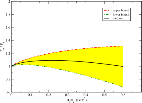
(a)

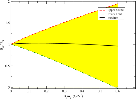
(b)

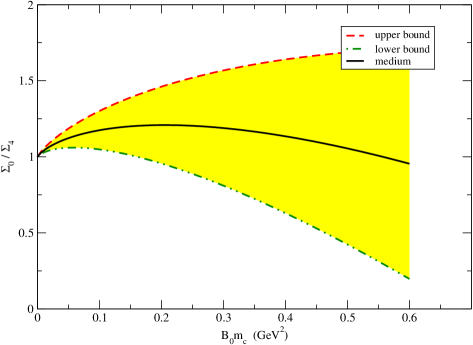
(c)

Figure 1: Plots for the ratios $F_{3}/F_{4}$, $B_{3}/B_{4}$ and $\Sigma_{3}/\Sigma_{4}$.

In addition, the relations (5.2) allow to determine the $m_{c}$–dependence of known $\chi$pt-results in pure $\mathrm{SU}(3)$–language at leading order from existing calculations. For example we obtain for $m_{u}=m_{d}=\hat{m}$

$$\partial_{m_{c}}\langle 0|\bar{q}q|0\rangle =B_{0}^{2}\left(2\nu_{D}+\tfrac{4}{9}\nu_{\eta_{c}}-32L_{6}^{\mathrm{r}}+\tfrac{82\hat{m}-7m_{s}}{m_{c}}\tfrac{1}{1152\pi^{2}}-\tfrac{1}{144\pi^{2}}\right)\,;\quad q\in\{u;d\}\,,$$ (6.2)

$$\partial_{m_{c}}F_{\pi} =\frac{B_{0}}{F_{0}}\left(-\nu_{D}+8L_{4}^{\mathrm{r}}-\tfrac{\hat{m}}{m_{c}}\tfrac{1}{32\pi^{2}}\right)\,,$$ (6.3)

$$\partial_{m_{c}}M_{\pi}^{2} =\frac{2B_{0}^{2}\hat{m}}{F_{0}^{2}}\left[-\tfrac{4}{9}\nu_{\eta_{c}}-16(L_{4}^{\mathrm{r}}-2L_{6}^{\mathrm{r}})-\tfrac{10\hat{m}-7m_{s}}{m_{c}}\tfrac{1}{576\pi^{2}}+\tfrac{1}{144\pi^{2}}\right]\,.$$ (6.4)

To obtain these expressions, all one has to do is to substitute the lecs in the corresponding $\mathrm{SU}(3)$–expressions[3] with the pertinent relations of (5.2) to arrive at explicit formulae for the light quark mass dependence with lecs that do not depend on these masses. Afterwards, one can directly differentiate the formulae by $m_{c}$ and apply the relations (5.2) again to obtain expressions in the $\mathrm{SU}(3)$–language. The dependence for other quantities can easily obtained by this procedure form the existing literature.

7    Summary

To summarise, we have determined the dependence on the $N^{\text{th}}$ quark mass of the $N-1$–flavour lecs $B_{N-1}$ and $F_{N-1}$ to next–to-leading and of the lecs $L_{0}^{N-1},\ldots,L_{12}^{N-1}$ to leading order. The calculation relied on a matching between the local parts of the generating functionals of $\chi$pt_N and $\chi$pt_N-1. We hence showed that the same procedure used for the determination of the strange quark mass dependence[6, 7, 10] of the two–flavour lecs can be generalised to the case with an arbitrary number of flavours.

These relations are useful to obtain constraints and further information on the pertinent lecs. We applied the relations to obtain the $m_{c}$–dependence of the quark condensate in a limit where the mass of the charm quark is well below half a GeV. This relation could be used in lattice calculations as an additional analytic anchor in an unphysical regime.

a    Notation

In this appendix, we will settle the notation of $\chi$pt_N, as this work is written in Euclidean spacetime throughout.

Chiral perturbation theory yields a consistent and systematic framework to explore the effects of symmetries in low energy qcd. The starting point is the massless qcd–Lagrangian $\mathcal{L}_{\text{\sc qcd\rm{}}}^{0}$, enriched with couplings to external (axial–) vector fields ($a_{\mu}$) $v_{\mu}$ and (pseudo–) scalar sources ($p$) $s$.

Chiral perturbation theory is formulated with the aid of an effective Lagrangian $\mathcal{L}_{\text{$\chi$\sc pt\rm{}}}=\sum_{n}\mathcal{L}_{2n}$, where the degrees of freedom are the emerging Goldstone bosons – identified with the light mesons – due to the spontaneous symmetry breakdown inherent to $\mathcal{L}_{\text{\sc qcd\rm}}^{0}$. The Lagrangian densities $\mathcal{L}_{2n}$ are organised in a counting scheme that allows for an expansion in the external momentum and the symmetry breaking terms.

The mesons are described in a Hermitian traceless field $\phi^{N}$, spanned by a basis of $N^{2}-1$ dimensions with elements $\{\lambda^{N}_{a}\}$, such that $\phi^{N}=\phi^{N}_{a}\lambda^{N}_{a}$ (implicit summation over repeated indices is assumed). As an explicit representation, we choose one related to the fundamental representation, but normalised as $\langle\lambda_{a}^{N}\lambda_{b}^{N}\rangle=2\delta_{ab}$. There are $N-1$ purely diagonal elements

$$\lambda_{n}^{N}=\sqrt{\frac{2}{n(n-1)}}\;\mathrm{diag}\big{(}1_{n-1},1-n,0_{N-n}\big{)}\,;\qquad 2\leq n\leq N\,,$$

and $N(N-1)$ purely off–diagonal sparse Hermitian elements

$$\lambda_{nk}^{N}=i^{k\!\!\!\!\!\mod 2}\,e_{n\lceil k/2\rceil}+(-i)^{k\!\!\!\!\!\mod 2}\,e_{\lceil k/2\rceil n}\,;\quad n\in\{2;3;\ldots;N\}\,,k\in\{1;2;\ldots;2(n-1)\}\,.$$

With $e_{kn}$ we denote the matrix whose only nonvanishing entry is a 1 in the $k^{\text{th}}$ row and $n^{\text{th}}$ column. The particles described with these matrices and their interactions considered below motivate to define the following three subsets of the basis: The element $\lambda_{N}^{N}$ will be denoted by $\lambda_{\eta}$, the $2(N-1)$ elements with entries only in the $N^{\text{th}}$ row and column will be addressed by the set $\lambda_{K}$ and all others by the set $\lambda_{\pi}$. This will simplify the notation in the following, as the corresponding collection of particles are addressed with the same labels $\eta$, $K$, and $\pi$. Any basis of traceless Hermitian $N\times N$-matrices with the above norm fulfils the completeness relation

$$\sum_{a=1}^{N^{2}-1}(\lambda^{N}_{a})_{kl}(\lambda^{N}_{a})_{mn}=2\delta_{kn}\delta_{lm}-\tfrac{2}{N}\delta_{kl}\delta_{mn}\,,$$ (a.1)

which we will make use of later.

We use a representation of the chiral symmetry where the operators $X$ of the Lagrangian transform under chiral rotations $g=(g_{L},g_{R})\in\mathrm{SU}(N)_{L}\times\mathrm{SU}(N)_{R}$ as

$$X\rightarrow f(g,\phi^{N})Xf(g,\phi^{N})^{-1}\,.$$ (a.2)

The compensator field $f$ is defined via the nonlinear representation of the meson field $u^{N}(\phi^{N})$ under the action of $g$ as

$$u^{N}(\phi^{N})\rightarrow u^{N}(\phi^{N}{}^{\prime})=g_{R}u^{N}(\phi^{N})f(g,\phi^{N})^{-1}=f(g,\phi^{N})u^{N}(\phi^{N})g_{L}{}^{-1}\,.$$

This representation is related to the customary $LR$–view via $U^{N}=(u^{N})^{2}$, where conventionally the explicit form of $U^{N}$ reads $U^{N}=\exp{(i\phi^{N}/F_{N})}$, with $F_{N}$ being one of the two low-energy constants of the leading Lagrangian $\mathcal{L}_{2}$, carrying the dimension of mass.

The elementary building blocks transforming as (a.2), used for building the Lagrangians $\mathcal{L}_{2}^{N}$ and $\mathcal{L}_{4}^{N}$, are given by

$$\begin{split}u^{N}_{\mu}&=i\left[u^{N}{}^{\dagger}(\partial_{\mu}-ir^{N}_{\mu})u^{N}-u^{N}(\partial_{\mu}-il^{N}_{\mu})u^{N}{}^{\dagger}\right]\,,\\ \chi^{N}_{\pm}&=u^{N}{}^{\dagger}\chi^{N}u^{N}{}^{\dagger}\pm u^{N}\chi^{N}{}^{\dagger}u^{N}\,,\\ f^{N}_{\pm\mu\nu}&=u^{N}l^{N}_{\mu\nu}u^{N}{}^{\dagger}\pm u^{N}{}^{\dagger}r^{N}_{\mu\nu}u^{N}\,,\end{split}$$ (a.3)

where the following combinations of (axial–) vector sources

$$r^{N}_{\mu}=v^{N}_{\mu}+a^{N}_{\mu}\,,\quad l^{N}_{\mu}=v^{N}_{\mu}-a^{N}_{\mu}\,,\\$$

and their field strengths

$$r^{N}_{\mu\nu} =\partial_{\mu}r^{N}_{\nu}-\partial_{\nu}r^{N}_{\mu}-i[r^{N}_{\mu},r^{N}_{\nu}]\,,$$

$$l^{N}_{\mu\nu} =\partial_{\mu}l^{N}_{\nu}-\partial_{\nu}l^{N}_{\mu}-i[l^{N}_{\mu},l^{N}_{\nu}]\,,$$

as well as the (pseudo–) scalar source combination

$$\chi^{N}=2B_{N}(s^{N}+ip^{N})\,,$$

have been introduced. Written in these building blocks, the leading order Lagrangian reads

$$\mathcal{L}_{2}^{N}=\frac{F_{N}^{2}}{4}\langle u^{N}\cdot u^{N}-\chi^{N}_{+}\rangle\,.$$ (a.4)

This Lagrangian implies the equations of motion

$$\nabla^{N}_{\mu}u^{N}_{\mu}+\tfrac{i}{2}\tilde{\chi}^{N}_{-}=0\,,$$ (a.5)

where $\tilde{\chi}^{N}_{-}$ denotes the traceless part of $\chi^{N}_{-}$ and the covariant derivative $\nabla^{N}_{\mu}$ is defined in terms of the chiral connection $\Gamma_{\mu}^{N}$ as

$$\begin{split}\nabla^{N}_{\mu}\cdot{}&=\partial_{\mu}\cdot{}+\,[\,\Gamma_{\mu}^{N}\,,\,\cdot{}\;]\qquad\text{with}\\ \Gamma_{\mu}^{N}&=\tfrac{1}{2}\left[u^{N}{}^{\dagger}(\partial_{\mu}-ir^{N}_{\mu})u^{N}+u^{N}(\partial_{\mu}-il^{N}_{\mu})u^{N}{}^{\dagger}\right]\,.\end{split}$$ (a.6)

The generating functional $Z_{N}$ can be written in a series where the elements are ordered by the number of loops involved in their determination. This series is equivalent to reintroduce the old–fashioned $\hbar$ and expanding $Z$ in powers of $\hbar$. The formal derivation of this series relies on splitting the field $\phi$ into the part fulfilling the equations of motion $\phi_{\text{cl}}$ and a quantum fluctuation $\xi$, parametrised as

$$U^{N}(\phi)=u^{N}_{\text{cl}}\,\exp\frac{i\xi}{F_{N}}\;u^{N}_{\text{cl}}\,;\qquad u^{N}_{\text{cl}}=u^{N}(\phi^{N}_{\text{cl}})\,.$$

Counting $\xi$ as a quantity of order $\hbar^{1/2}$ and expanding the formal representation of $Z_{N}$ as a path integral in powers of $\hbar$ delivers the desired loop expansion,

$$Z^{N}=\bar{S}_{2}^{N}+\hbar\left(\bar{S}_{4}^{N}+\tfrac{1}{2}\ln\det D^{N}/D_{0}^{N}\right)+O\!\left(\hbar^{2}\right)\,,$$

where $\bar{S}_{n}^{N}$ denotes the classical action belonging to $\mathcal{L}_{n}^{N}$ and the differential operator $D^{N}$ is given in $\chi$pt_N as

$$D^{N}(x)=-d_{x}^{2}+\sigma^{N}(x)\,;\qquad d^{x}_{\mu}=\partial^{x}_{\mu}+\hat{\Gamma}^{N}_{\mu}(x)\,;\qquad\left(D_{0}^{N}\right)_{ab}=-\delta_{ab}\left(\Delta+\bar{M}_{a}^{2}\right)\,,$$ (a.7)

with

$$\begin{split}\hat{\Gamma}^{N}_{\mu}{\,}_{ab}&=-\tfrac{1}{2}\langle[\lambda^{N}_{a},\lambda^{N}_{b}]\Gamma^{N}_{\mu}\rangle\,,\\ \sigma^{N}_{ab}&=\tfrac{1}{8}\langle[\lambda^{N}_{a},u^{N}_{\mu}][\lambda^{N}_{b},u^{N}_{\mu}]\rangle+\tfrac{1}{8}\langle\{\lambda^{N}_{a},\lambda^{N}_{b}\}\chi^{N}_{+}\rangle\,.\end{split}$$ (a.8)

The Lagrangian $\mathcal{L}_{4}^{N}$ is given as

$$\mathcal{L}_{4}^{N}=\sum_{j=0}^{12}L^{N}_{j}X^{N}_{j}\,,$$ (a.9)

with lecs $L^{N}_{j}$. The corresponding operators $X^{N}_{j}$ read[3]

$$\begin{split}X^{N}_{0}&=-\langle(u^{N}_{\mu}u^{N}_{\nu})^{2}\rangle\,,&&\\ X^{N}_{1}&=-\langle u^{N}\cdot u^{N}\rangle^{2},&\qquad X^{N}_{2}&=-\langle u^{N}_{\mu}u^{N}_{\nu}\rangle^{2}\,,\\ X^{N}_{3}&=-\langle(u^{N}\cdot u^{N})^{2}\rangle,&\qquad X^{N}_{4}&=\langle u^{N}\cdot u^{N}\rangle\langle\chi^{N}_{+}\rangle\,,\\ X^{N}_{5}&=\langle u^{N}\cdot u^{N}\,\chi^{N}_{+}\rangle,&\qquad X^{N}_{6}&=-\langle\chi^{N}_{+}\rangle^{2}\,,\\ X^{N}_{7}&=-\langle\chi^{N}_{-}\rangle^{2},&\qquad X^{N}_{8}&=-\tfrac{1}{2}\langle(\chi^{N}_{+})^{2}+(\chi^{N}_{-})^{2}\rangle\,,\\ X^{N}_{9}&=\tfrac{i}{2}\langle f^{N}_{+\mu\nu}[\,u^{N}_{\mu}\,,\,u^{N}_{\nu}\,]\rangle,&\qquad X^{N}_{10}&=-\tfrac{1}{4}\langle(f^{N}_{+})^{2}-(f^{N}_{-})^{2}\rangle\,,\\ X^{N}_{11}&=-\tfrac{1}{2}\langle(f^{N}_{+})^{2}+(f^{N}_{-})^{2}\rangle,&\qquad X^{N}_{12}&=-\tfrac{1}{4}\langle(\chi^{N}_{+})^{2}-(\chi^{N}_{-})^{2}\rangle\,.\end{split}$$ (a.10)

We used the abbreviations $u^{N}\cdot u^{N}=u^{N}_{\mu}u^{N}_{\mu}$ and $(f^{N}_{\pm})^{2}=f^{N}_{\pm\mu\nu}f^{N}_{\pm\mu\nu}.$

b    Tree-level

In this appendix we will point out the details of the tree–level contribution calculation to the generating functional. As pointed out in Section 4, the calculation involves the following steps:

• show that $u^{N}$ is of the form (4.1)

• express the $\eta$ in terms of $\mathrm{SU}(N-1)$–fields

• show that the $\pi$ do not differ from those in $\mathrm{SU}(N-1)$ at the required order

To see the triviality of the classical $K$–fields, we observe that in our $N-1$–flavour limit the only fields proportional to elements in $\lambda_{K}$ are the $K$–fields themselves. All other fields and sources are proportional to a combination of elements of $\lambda_{\pi}$, $\lambda_{\eta}$, or unity. Under the linear transformation $\lambda_{a}^{N}\mapsto S\lambda_{a}^{N}S^{-1}$, with $S=\operatorname{diag}(1_{N-1},\,-1)$, $\lambda_{\pi}$ and $\lambda_{\eta}$ are invariant, whereas the elements of $\lambda_{K}$ pick up a minus sign. However, $\mathcal{L}_{2}$ as a trace is invariant under the same transformation, therefore also the equations of motion. Hence there can be only vertices emitting an even number of $K$–lines. The invariance of the Lagrangian under this transformation indicates a conservation law, known for $N=3$ as strangeness conservation.

But tree graphs containing $K$–particles cannot solely consist of vertices with an even number of $K$–lines attached, as e.g. the endpoints of the $K$–branches of the tree have only one. Hence there are no tree graphs with $K$–content in our $N-1$–flavour limit and the solution of the equations of motion of the mesons can be written as a (commuting) combination of $\pi$– and $\eta$–fields:

$${u^{N}}=u^{\pi}e^{\tfrac{i}{2F_{N}}{\eta}\lambda_{\eta}}\,.$$ (b.1)

Note that the field $u^{\pi}$ does not (necessarily) equal to $u^{N-1}$ of $\chi$pt_N-1, since it fulfils the equations of motion for the $\mathrm{SU}(N)$ version, which are different from the ones in the $N-1$–flavour case (see below).

Exploiting the simplification of the $N-1$–flavour limit in the representation of the solution of the equations of motion, we may write the building blocks of the Lagrangian $\mathcal{L}^{N}_{2}$ as

$$\begin{split}u^{N}_{\mu}&=u^{\pi}_{\mu}-\tfrac{1}{F_{N}}\lambda_{\eta}\partial_{\mu}\eta\,,\\ \chi^{N}_{\pm}&=\frac{B_{N}}{B_{N-1}}\left(\chi^{\pi}_{\pm}\cos\alpha-i\chi_{\mp}^{\pi}\sin\alpha\right)+4B_{N}m\,e_{NN}\begin{cases}\phantom{i}\cos(N-1)\alpha&\quad{\chi}_{+}^{N}\\ i\sin(N-1)\alpha&\quad{\chi}_{-}^{N}\end{cases}\,,\\ \end{split}$$ (b.2)

with $\alpha=\sqrt{2/[N(N-1)]}\,\eta/F_{N}$ and operators $X^{\pi}$ denote $X$ evaluated with the fields $u^{\pi}$ and in the external fields only the $\mathrm{SU}(N-1)$–part being different from zero, $B_{N}$ replaced by $B_{N-1}$. The only nonzero entry of the matrix $e_{NN}$ consists of a 1 in the lower right corner. As will be shown in a moment, $\alpha$ is a quantity of order $q^{2},$ therefore we may expand the trigonometric functions for small $\alpha$ and obtain a perturbation series up to a given order. Remarkably, the leading term of the expansion of $\chi_{+}^{N}$ is not its $\mathrm{SU}(N-1)$ equivalent, but rather the mass term $4B_{N}me_{NN}$, which has a counting of $q^{0}$ and $\hbar^{-1}$. As we will see, this has the effect that higher order terms of the $N$–flavour functional contribute also to the leading term of the $N-1$–flavour theory.

Expressing the Lagrangian $\mathcal{L}_{2}^{N}$ in these terms, we can write down the equation of motion for the $\eta$–particle as

$$\begin{split}\left(\Delta-\bar{M}_{\eta}^{2}\right)\eta&=-\bar{M}_{\eta}^{2}\eta+F_{N}B_{N}m\sqrt{\frac{2(N-1)}{N}}\sin(N-1)\alpha\\ &+\frac{F_{N}}{4}\frac{B_{N}}{B_{N-1}}\sqrt{\frac{2}{N(N-1)}}\left[\sin\alpha\langle\chi_{+}^{l}\rangle+i\cos\alpha\langle\chi_{-}^{l}\rangle\right]\,,\end{split}$$ (b.3)

which can be solved for small $\alpha$ recursively. Note that the sum of the first two terms on the right hand side is of the order $\alpha^{3}$ in the expansion for small $\alpha$ when inserting the tree-level mass (3.1). Therefore, the inclusion of the $\eta$–mass term on the left hand side is natural. The differential equation suggests a counting in which every occurrence of an $\eta$–particle should count as $q^{2}$. We may now solve this equation recursively for small momenta, respecting the counting, and find

$$\eta=-\frac{iF_{N}}{8B_{N-1}m}\sqrt{\frac{2N}{(N-1)^{3}}}\langle\chi^{\pi}_{-}\rangle+O(q^{4})\,.$$ (b.4)

For the equations of motion of the $\pi$-particles we note that they are different in the two theories in question,

$$\mathrm{SU}(N) : \nabla_{\mu}^{\pi}u_{\mu}^{\pi} =-\tfrac{i}{2}\tfrac{B_{N}}{B_{N-1}}\left(\tilde{\chi}_{-}^{\pi}\cos\alpha-i\tilde{\chi}_{+}^{\pi}\sin\alpha\right)\,,\qquad\qquad\qquad\qquad\qquad$$

$$\mathrm{SU}(N-1) : \nabla_{\mu}^{N-1}u_{\mu}^{N-1} =-\tfrac{i}{2}\tilde{\chi}_{-}^{N-1}\,.$$

However, the difference is only a quantity of order $q^{4}$, therefore we can assume for our application that the solutions are the same, i.e. fields with index $\cdot^{\pi}$ are equivalent to fields with index $\cdot^{N-1}$.

The counterterm contribution of $\mathcal{L}^{N}_{4}$ is evaluated at the solution of the equation of motion also, therefore we can use the same technique to find its representation in $\chi$pt_N-1. This can be achieved by using the following translation rule:

$${f}_{\pm\mu\nu}^{N}\rightarrow f^{\pi}_{\pm\mu\nu}\,,$$ (b.5)

to be understood to give the correct corresponding local term in the action $\int\!\mathrm{d}^{d}x\,\mathcal{L}_{4}^{N}$.

c    Loops at order $\hbar$

Having translated the tree-level part of the functional, we turn to the loop terms of order $\hbar.$ Here we calculate again the contribution to the $\mathrm{SU}(N)$–functional in our $N-1$–flavour limit to see how it is included in pure $\chi$pt_N-1. It remains to calculate the local contributions of

$$Z_{1\,\mathrm{loop}}^{N}=\tfrac{1}{2}\ln\frac{\det D^{N}}{\det D^{N}_{0}}\,.$$

Following the work of Nyffeler and Schenk [19] and exploiting the simplifications due to the $N-1$–flavour limit we are considering here [$K$–particles do not mix with the others, consult (a.7)], the determinant can be written as

$$\ln\det D^{N}=\ln\det D_{\pi}+\ln\det D_{\eta}+\ln\det D_{K}+\ln\det(1-D_{\pi}^{-1}D_{\pi\eta}D_{\eta}^{-1}D_{\eta\pi})\,,$$ (c.1)

where the index of $D^{N}$ denotes the subspace to consider. Note that the inverses of the sub-blocks of $D^{N}$ do not correspond to the propagators, since they do not include any mixing terms among massive and massless particles. However, this makes them perfect candidates for a treatment via heat–kernel techniques (for more detail consult [19] and the references therein). The mixing is here explicitly present in the last term. We will now investigate each of these terms in turn.

Following the argument that the corrections to the massless fields are automatically generated by the generating functional of an effective Lagrangian, we can neglect the part involving only $\pi$–particles, since it will produce in the end the same terms as its $\mathrm{SU}(N-1)$ counterpart and will hence be purely nonlocal.

The next two determinants describe tadpoles with insertions where only particles of identical masses run in the loop: either $K$– or $\eta$–particles. Diagrams of this type can be represented (with internal tree–level mass $z$) as

$$\ln\frac{\det D_{z}}{\det D_{0}}=-\sum_{n=1}^{\infty}\Gamma(n)F_{n}(z^{2})\operatorname{Tr}\big{(}a_{n}\big{)}\,,\qquad F_{n}(z^{2})=\int\!\frac{\mathrm{d}^{d}\ell}{(2\pi)^{d}}\,(z^{2}+\ell^{2})^{-n}\,.$$ (c.2)

The first two Seeley-coefficients $a_{1}$ and $a_{2}$ are given as (with $\bar{\sigma}=\sigma-z^{2}$)

$$a_{1}=-\bar{\sigma}\,,\qquad a_{2}=\tfrac{1}{2}\bar{\sigma}^{2}-\tfrac{1}{6}\hat{\nabla}^{2}\bar{\sigma}+\tfrac{1}{12}\hat{\Gamma}_{\mu\nu}\hat{\Gamma}_{\mu\nu}\,,$$

where the field strength $\hat{\Gamma}_{\mu\nu}=[d_{\mu}\,,\,d_{\nu}]$ and the differential $\hat{\nabla}_{\mu}\,\cdot=\partial_{\mu}\cdot\,+\,[\,\hat{\Gamma}_{\mu}\,,\,\cdot\,]$. Note that each $a_{n}$ in the series is suppressed by an order $q^{2}$ to its predecessor, therefore the method is tailored to our counting scheme. The trace $\operatorname{Tr}$ is understood as a simultaneous ordinary trace and an integral over position space.

At order $q^{4}$, we get

$$\ln\frac{\det D_{K}}{\det D^{0}_{K}} =F_{1}(\bar{M}_{K}^{2})\operatorname{Tr}_{K}(\bar{\sigma})-\tfrac{1}{12}F_{2}(\bar{M}_{K}^{2})\operatorname{Tr}_{K}(6\bar{\sigma}^{2}+\hat{\Gamma}_{\mu\nu}\hat{\Gamma}_{\mu\nu})\,,$$ (c.3)

$$\ln\frac{\det D_{\eta}}{\det D^{0}_{\eta}} =F_{1}(\bar{M}_{\eta}^{2})\operatorname{Tr}_{\eta}(\bar{\sigma})-\tfrac{1}{2}F_{2}(\bar{M}_{\eta}^{2})\operatorname{Tr}_{\eta}(\bar{\sigma}^{2})\,.$$ (c.4)

The field strength $\hat{\Gamma}_{\mu\nu}$ vanishes in the $\eta$–case. Also note that the second term of $a_{2}$ is a total derivative and can therefore be dropped. With $\operatorname{Tr}_{P}$ we denote the partial flavour trace over the flavour subspace spanned by the particle $P$ and an integral over position space.

In the above expressions, the only obstacle to overcome is the calculation of the flavour traces. For the case of the $\eta$–particle, the trace is trivial as here the Seeley–coefficients are one–dimensional. In the case of the $K$–particle, however, matters are more involved. Formally, the problem is to calculate the partial flavour trace over a product of matrices $X_{ab}=X^{1}_{ac_{1}}\cdots X^{n+1}_{c_{n}b}$, where all indices are assumed to run only over the subspace spanned by the $K$–particles. For the outer indices $a$ and $b$, the solution is to calculate $\operatorname{Tr}_{K}=\operatorname{Tr}_{N}-\operatorname{Tr}_{N-1}-\operatorname{Tr}_{\eta}$. For the inner indices, observe that in our $N-1$ flavour limit, any component $X^{k}_{c_{k-1}c_{k}}$ with exactly one index in the $K$–space vanishes. Therefore, the inner summation can be carried out over all $\mathrm{SU}(N)$. Hence, all one needs to know is to calculate the trace over the whole $\mathrm{SU}(N)$. This can be carried out the via the completeness relation (a.1). From this relation follows that

$$\begin{split}\sum_{a=1}^{N^{2}-1}\langle\lambda^{N}_{a}A\lambda^{N}_{a}B\rangle&=-\tfrac{2}{N}\langle AB\rangle+2\langle A\rangle\langle B\rangle\qquad\text{and}\\ \sum_{a=1}^{N^{2}-1}\langle\lambda^{N}_{a}A\rangle\langle\lambda^{N}_{a}B\rangle&=2\langle AB\rangle-\tfrac{2}{N}\langle A\rangle\langle B\rangle\,.\end{split}$$ (c.5)

As the components of the Seeley–coefficients are given in (a.8) in exactly this basis, the traces can be determined mechanically.

The last term of Equation (4.4) behaves somewhat differently, as it contains two different propagators. We write

$$\ln\det(1-D_{\pi}^{-1}D_{\pi\eta}D_{\eta}^{-1}D_{\eta\pi})=-\operatorname{Tr}(D_{\pi}^{-1}D_{\pi\eta}D_{\eta}^{-1}D_{\eta\pi})+\text{non--local terms.}$$ (c.6)

Note that already the first term of an expansion in the interaction of the determinant yields all local contributions. Of course, the contained propagators still have to be expanded via the heat–kernel techniques, but one has no longer to bother which terms of the mixing contribution are local and which aren’t. At order $q^{4}$, the propagators amount just to their free variants and the mixing vertex is $\bar{\sigma}_{\eta\pi}$.

The flavour traces and the translation of the vertices into terms of the $N-1$–flavour theory can be performed by the same methods as in the tree–level calculation.

All in all, the local contribution to $Z_{\text{1loop}}^{N}$ is of the form (4.5)

For the occurring loop–integrals, we use the $\overline{\text{MS}}$–scheme for their renormalisation. Multiplying the $d$–dimensional loop–integrals with a factor $(\mu c)^{-2\omega}$ yields the correct mass dimension when performing the transition to four space–time dimensions. Here, we introduced an arbitrary mass scale $\mu$ and a constant $c$ that is conventionally chosen such that

$$\ln c=-\tfrac{1}{2}[\ln 4\pi+\Gamma^{\prime}(1)+1]\,.$$

The variation from four to $d$ space–time dimensions is contained in

$$\omega=d/2-2\,.$$

A Laurent–expansion of the resulting expressions around $\omega=0$ and dropping the principal part yields the normalised results for the loop–integrals.

In $d$ dimensions, the needed loop–integrals read

$$\begin{split}F_{n}^{m}(z)&=\int\!\frac{\mathrm{d}^{d}\ell}{(2\pi)^{d}}\,\ell^{-2m}(z+\ell^{2})^{m-n}\,,\qquad n>m\geq 0\,,\qquad F_{n}(z)=F_{n}^{0}(z)\,;\\ &=z^{\omega+2-n}\,C(\omega)\,\frac{\Gamma(\omega+2-m)\Gamma(n-2-\omega)}{\Gamma(\omega+2)\Gamma(n-m)}\,,\qquad C(\omega)=(4\pi)^{-(2+\omega)}\,.\end{split}$$ (c.7)

d    Validity for $N=3$

In this short appendix, we spell out the details of the check that our results correspond to the ones already known for $N=3$ [3].

Eliminating $X_{0}^{3}$ in the list of operators yields already the standard minimal basis for $N=3$. Therefore, putting $L_{0}^{\mathrm{r}}{}^{3}=0$ in the results (5.2) deals with the nonminimality of (a.10) for $N=3$. Note that this still leaves a loop contribution to $L_{0}^{\mathrm{r}}{}^{2}$, as a kaon-loop with two insertions still produces a local contribution proportional to $X_{0}^{2}$, as can be seen from (4.6).

The Cayley-Hamilton relation for two-dimensional matrices $A$ and $B$,

$$\{A\,,\,B\}=A\langle B\rangle+\langle A\rangle B+\langle AB\rangle-\langle A\rangle\langle B\rangle\,,$$

can be used to yield a minimal basis for $N=2$ in the form of a reduced set of (a.10). In that manner we eliminate the elements $X_{0}^{2}$, $X_{3}^{2}$, and $X_{5}^{2}$; i.e. $X_{l}^{2}=\beta_{lk}X_{k}^{2}{}^{\text{min}}$. All remaining operators $X_{k}^{2}{}^{\text{min}}$ except for $X_{4}^{2}$ can be transformed into the standard basis elements $K_{j}$ of $\chi$pt₂[2] as linear combinations,

$$K_{1} =-\tfrac{1}{4}\langle u\cdot u\rangle^{2}, \qquad K_{2} =-\tfrac{1}{4}\langle u_{\mu}u_{\nu}\rangle^{2}\,,$$

$$K_{3} =-\tfrac{1}{16}\langle\chi_{+}\rangle^{2}, \qquad K_{4} =\tfrac{i}{4}\langle u_{\mu}\chi_{-\mu}\rangle\,,$$

$$K_{5} =\tfrac{1}{2}\langle f_{-}^{2}\rangle, \qquad K_{6} =-\tfrac{i}{4}\langle f_{+\mu\nu}[\,u_{\mu}\,,\,u_{\nu}\,]\rangle\,,$$

$$K_{7} =\tfrac{1}{16}\langle\chi_{-}\rangle^{2}, \qquad X_{8} =-\tfrac{1}{8}(\det\chi_{+}+\det\chi_{-})\,,$$

$$K_{9} =\langle f_{+}^{2}+f_{-}^{2}\rangle\,, \qquad K_{10} =-\tfrac{1}{16}\langle\chi_{+}^{2}-\chi_{-}^{2}\rangle\,.$$

For simplicity, we neglected the superscript $\cdot^{2}$ to indicate that here $N=2$ and introduced the notation $\chi_{\pm\mu}=\nabla_{\mu}\chi_{\pm}-\tfrac{i}{2}\{\chi_{\mp},u_{\mu}\}$. In this notation, $\mathcal{L}_{4}=\sum_{j=1}^{10}l_{j}K_{j}$, where the commonly used $h_{i}$ translate to $h_{1}-h_{3}=l_{8}$, $h_{2}=l_{9}$, and $h_{3}=l_{10}$.

The element $X_{4}^{2}$ can be written as a combination of $K_{4}$ and other $K_{j}$ by the use of the equations of motion. As the operators of the basis enter the generating functional only at the point where the contained fields satisfy the equations of motion, this is not an issue. One obtains in this manner a list of transformation equations of the form $X_{k}^{2}{}^{\text{min}}=\alpha_{kj}K_{j}$. The contribution to a specific lec $l_{j}^{\mathrm{r}}$ is then given by $l_{j}^{\mathrm{r}}=\beta_{lk}\alpha_{kj}L_{l}^{\mathrm{r}}{}^{2}$, where for $L_{l}^{\mathrm{r}}{}^{2}$ the solutions of (5.2) are inserted.

References

• [1] S. Weinberg, “Phenomenological Lagrangians”, Physica A96 (1979), 327.
• [2] J. Gasser and H. Leutwyler, “Chiral perturbation theory to one loop”, Ann. Phys. 158 (1984), 142.
• [3] J. Gasser and H. Leutwyler, “Chiral perturbation theory: Expansions in the mass of the strange quark”, Nucl. Phys. B250 (1985), 465.
• [4] B. Moussallam, “Flavor stability of the chiral vacuum and scalar meson dynamics”, JHEP 08 (2000), 005, hep-ph/0005245.
• [5] R. Kaiser and J. Schweizer, “The expansion by regions in $\pi K$ scattering”, JHEP 06 (2006), 9, hep-ph/0603153.
• [6] J. Gasser, C. Haefeli, M. A. Ivanov, et al., “Integrating out strange quarks in ChPT”, Phys. Lett. B652 (2007), 21, 0706.0955.
• [7] J. Gasser, C. Haefeli, M. A. Ivanov, et al., “Integrating out strange quarks in ChPT: terms at order $p^{6}$”, Phys. Lett. B675 (2009), 49, 0903.0801.
• [8] J. Gasser, V. E. Lyubovitskij, A. Rusetsky, et al., “Decays of the $\pi_{+}\,\pi_{-}$ atom”, Phys. Rev. D64 (2001), 16008, hep-ph/0103157.
• [9] H. Jallouli and H. Sazdjian, “Relativistic effects in the pionium lifetime”, Phys. Rev. D58 (1998), 014011, hep-ph/9706450.
• [10] C. Haefeli, M. A. Ivanov, and M. Schmid, “Electromagnetic low-energy constants in ChPT”, Eur. Phys. J. C53 (2008), 549, 0710.5432.
• [11] K. Kampf and B. Moussallam, “Chiral expansions of the $\pi_{0}$ lifetime”, 0901.4688.
• [12] M. Schmid, Strangeless $\chi$PT at large $m_{s}$, Ph.D. thesis, University of Bern (2007).
• [13] J. Bijnens, G. Colangelo, and G. Ecker, “Renormalization of Chiral Perturbation Theory to Order $p^{6}$”, Annals Phys. 280 2000, 100, hep-ph/9907333
• [14] S. Descotes-Genon, L. Girlanda, and J. Stern, “Paramagnetic effect of light quark loops on chiral symmetry breaking”, JHEP 01 (2000), 041, hep-ph/9910537.
• [15] S. Descotes-Genon, L. Girlanda, and J. Stern, “Chiral order and fluctuations in multi-flavour QCD”, Eur. Phys. J. C27 (2003), 115, hep-ph/0207337.
• [16] S. Descotes-Genon, N. H. Fuchs, L. Girlanda, et al., “Resumming QCD vacuum fluctuations in three-flavour chiral perturbation theory”, Eur. Phys. J. C34 (2004), 201, hep-ph/0311120.
• [17] S. Descotes-Genon, “$\pi$-$\pi$ and $\pi$-$K$ scatterings in three-flavour resummed chiral perturbation theory”, J. Phys. Conf. Ser. 110 (2008), 052012, 0710.1696.
• [18] D. G. Boulware and L. S. Brown, “Tree graphs and classical fields”, Phys. Rev. 172 5 (1968), 1628.
• [19] A. Nyffeler and A. Schenk, “Effective field theory of the linear $\mathrm{O}(N)$ sigma model”, Annals Phys. 241 (1995), 301, hep-ph/9409436.
• [20] P. Hernandez and M. Laine, “Charm mass dependence of the weak Hamiltonian in chiral perturbation theory”, JHEP 0409 (2004), 018, hep-ph/0407086.