Coupled-cluster calculations for the ground- and excited-states of the spin-half XXZ model

Abstract

The coupled-cluster method is applied to the spin-1/2 antiferromagnetic XXZ model on a square lattice by employing an approximation which contains two-body long-range correlations and high-order four-body local correlations. Improvement is found for the ground-state energy, sublattice magnetization, and the critical anisotropy when comparing with the approximation including the two-body correlations alone. We also obtain the full excitation spectrum which is in good agreement with the quantum Monte Carlo results and the high-order spin-wave theory.

1 Introduction

The coupled-cluster method (CCM) is one of the most precise microscopic formulations of quantum many-body theories [1, 2, 3, 4, 5, 6, 7, 8, 9]. There is a large number of successful applications of CCM to a wide range of physical and chemical systems. In particular, the applications of CCM to spin systems on discrete spatial lattices have produced one of the most accurate results [10, 11, 12, 13, 14, 15, 16, 17, 18, 19, 20]. Several approximation schemes have been developed for the application of the CCM to the spin lattice systems. Two such successful schemes are the so-called SUB$n$ scheme in which all correlations of any range for up to $n$ spins are retained and the localised LSUB$m$ scheme in which $m$ or fewer adjacent spin sites over all distinct locales on the lattice are retained. Other high-order localized approximation schemes such as DSUB$m$ [19] and LPSUB$m$ [20] have also been employed. Up to now, most recent studies have presented results for the high-order calculations mainly based on the LSUB$m$ scheme in which the long-range order correlations are ignored [13, 14, 15, 16, 17, 18, 19, 20]. In this paper we present results for the ground and excitation states for an antiferromagnetic square lattice by combining the SUB2 and LSUB4 approximation schemes (SUB2+LSUB4). Due to inclusion of the two-body long-range correlations, we are able to obtain improved results for the ground-state properties, including the critical value of the anisotropy, as well as the full excitation spectrum which is difficult to calculate by using the localised approximation scheme alone.

The spin-1/2 antiferromagnetic XXZ Heisenberg Hamiltonian in terms of spin rasing $s^{+}$ and lowering $s^{-}$ operators is given by,

$$H=\frac{1}{2}\sum_{\langle i,j\rangle}[s_{i}^{+}s_{j}^{-}+s_{i}^{-}s_{j}^{+}+2\Delta s_{i}^{z}s_{j}^{z}],$$ (1)

where $\Delta$ is the anisotropy and the sum on $\langle i,j\rangle$ runs over all the nearest neighbor pairs once. The isotropic Heisenberg model is given by $\Delta=1$. Classically, the ground-state of Eq. (1) is ferromagnetic, with all spins aligned along $z$-axis for all lattice when $\Delta\leq-1$; for $|\Delta|\leq 1$ it is antiferromagnetic for all bipartite lattice with all spins are aligned along some arbitrary direction in the $xy-$plane; for $\Delta\geq 1$ it is antiferromagnetic with spins aligned along ($\pm$) directions of the $z$-axis. The classical Néel ground state with all up-spins on one sublattice and all down-spins on the other is chosen to be the model state in our CCM calculation. In this article, as before, we use index $i$ to label sites of the down-spin sublattice and index $j$ for the up-spin sublattice. It is useful to introduce a transformation for the local spin axes of one sublattice. This is achieved by rotating all up-spins by $180^{\circ}$ around the $y-$axis and hence every spin of the system points down in the Néel model state with $s^{z}=-1/2$. This transformation is given by for all $j$-sublattice operators, $s^{\mp}=s^{x}\mp is^{y}\,\rightarrow-s^{\pm}$ and $s^{z}\rightarrow-s^{z}$. The Hamiltonian of Eq. (1) after the rotation is rewritten as,

$$H=-\frac{1}{2}\sum_{\langle i,j\rangle}[s_{i}^{+}s_{j}^{+}+s_{i}^{-}s_{j}^{-}+2\Delta s_{i}^{z}s_{j}^{z}].$$ (2)

The ket and bra ground states of the CCM are given in terms of correlation operators $S$ and $\tilde{S}$ a respectively,

$$|\Psi\rangle=e^{S}|\Phi\rangle,\quad\,\,\quad S=\sum_{I}{\cal S}_{I}C_{I}^{\dagger},$$ (3)

$$\langle\tilde{\Psi}|=\langle\Phi|\tilde{S}e^{-S},\,\,\,\,\,\,\tilde{S}=1+\sum_{I}{\tilde{\cal S}}_{I}C_{I},$$ (4)

where the model state $|\Phi\rangle$ is the rotated Néel state as mentioned earlier with all the spins pointing down, $C^{\dagger}_{I}$ and $C_{I}$ are the so-called configurational creation and destruction operators respectively with the nominal index $I$ labeling the multi-spin raising and lowering operators as,

$$\sum_{I}{\cal S}_{I}C^{\dagger}_{I}=\frac{1}{(n!)^{2}}\sum_{n=1}^{N/2}\sum_{i_{1},i_{2}...i_{n},j_{1},j_{2}...j_{n}}{\cal S}_{i_{1},i_{2}...i_{n},j_{1},j_{2}...j_{n}}s_{i_{1}}^{+}s_{i_{2}}^{+}...s_{i_{n}}^{+}s_{j_{1}}^{+}s_{j_{2}}^{+}...s_{j_{n}}^{+},$$ (5)

$$\sum_{I}{\cal\tilde{S}}_{I}C_{I}=\frac{1}{(n!)^{2}}\sum_{n=1}^{N/2}\sum_{i_{1},i_{2}...i_{n},j_{1},j_{2}...j_{n}}{\cal\tilde{S}}_{i_{1},i_{2}...i_{n},j_{1},j_{2}...j_{n}}s_{i_{1}}^{-}s_{i_{2}}^{-}...s_{i_{n}}^{-}s_{j_{1}}^{-}s_{j_{2}}^{-}...s_{j_{n}}^{-},$$ (6)

with the ket-and bra-state correlation coefficients ${\cal S}_{I}$ and $\tilde{\cal S}_{I}$ to be determined variationally as shown below. We note that the bra-state $\langle\tilde{\Psi}|$ and the ket-state $|\Psi\rangle$ are not manifestly hermitian conjugate to one another. The normalization conditions $\langle\tilde{\Psi}|\Psi\rangle\equiv\langle\Phi|\Psi\rangle\equiv\langle\Phi|\Phi\rangle\equiv 1$ is satisfied by construction. The ground-state Schrödinger equation, $H|\Psi\rangle=E_{g}|\Psi\rangle,$ can now be written as,

$$\hat{H}|\Phi\rangle=E_{g}|\Phi\rangle,$$ (7)

where the similarity-transformed Hamiltonian $\hat{H}$ can be written in terms of a series of nested commutations as,

$$\hat{H}=e^{-S}He^{S}=H+[H,S]+\frac{1}{2!}[[H,S],S]+\cdots.$$ (8)

The expectation value of an arbitrary operator ${\cal O}$ can be written as,

$$\bar{{\cal O}}=\langle\tilde{\Psi}|{\cal O}|\Psi\rangle=\langle\Phi|{\tilde{S}}e^{-S}{\cal O}e^{S}|\Phi\rangle=\bar{{\cal O}}(\{{\cal S}_{I},\tilde{\cal S}_{I}\}).$$ (9)

The correlation coefficients $\{{\cal S}_{I},\tilde{\cal S}_{I}\}$ are determined variationally by the following equations,

$$\frac{\delta\bar{H}}{\delta\tilde{\cal S}_{I}}=0\Rightarrow\langle\Phi|C_{I}e^{-S}He^{S}|\Phi\rangle=0,$$ (10)

$$\frac{\delta\bar{H}}{\delta{\cal S}_{I}}=0\Rightarrow\langle\Phi|\tilde{S}e^{-S}[H,C_{I}^{+}]e^{S}|\Phi\rangle=0.$$ (11)

In the followings we will consider a specific approximation, namely the SUB2+LSUB4 scheme as defined earlier, by a similar truncation in both $S$ and $\tilde{S}$.

2 Ground-state energy for the SUB2+LSUB4
approximation scheme

As mentioned in Introduction, the SUB2 approximation retains two-spin-flip configurations of all orders. In the SUB4 scheme, additional 4-spin correlations are also included. We hence write the SUB4 ket-state operators as,

$$S=\sum_{i,j}^{N/2}b_{i,j}s_{i}^{+}s_{j}^{+}+\frac{1}{4}\sum_{i_{1},i_{2},j_{1},j_{2}}^{N/2}g_{i_{1},i_{2};j_{1},j_{2}}s_{i_{1}}^{+}s_{i_{2}}^{+}s_{j_{1}}^{+}s_{j_{2}}^{+},$$ (12)

where $b_{i,j}$ and $g_{i_{1},i_{2};j_{1},j_{2}}$ are the two-spin-flip and four-spin-flip correlation coefficients respectively. The full SUB4 scheme equations were obtained before [11], but they are difficult to solve. Here we consider the SUB2+LSUB4 scheme which retains ten local configurations as shown in Fig. 1, in additional to the other two-body high-order coefficients of the SUB2 scheme.

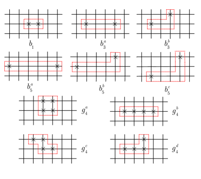
Figure 1: The graphical representation of the ten local configurations in Eqs. (17)-(20) for the short-range part of the SUB2+LSUB4 scheme. The flipped spins with respect to the Néel state are indicated by the crosses.

As described in general by Eq. (10), the SUB4 approximation consists of two sets of equations, the two-spin-flip and four-spin-flip equations. The two-spin-flip equations are given by,

$$\langle\Phi|s_{i}^{-}s_{j}^{-}e^{-S_{SUB4}}He^{S_{SUB4}}|\Phi\rangle=0,$$ (13)

from which we obtain the subset of the SUB2+LSUB4 approximation as,

$$\sum_{\rho}\big{[}(1+2\Delta b_{1} +2b_{1}^{2}+G_{1})\delta_{r,\rho}+2(\Delta+2b_{1})b_{r}$$

$$+G_{2}\delta_{r,\rho_{3a}}+G_{3}\delta_{r,\rho_{3b}}+\sum_{r^{\prime}}b_{r^{\prime}+\rho+\rho_{0}}b_{r-r^{\prime}-\rho_{0}}\big{]}=0,$$ (14)

where $\rho$ is the nearest-neighbor index vector with four possible values for a square lattice, $\rho_{0}$ is any one of them, $G_{\alpha}$ with $\alpha=1,2,3$ are defined as,

$$G_{1}=2g_{4}^{a}+2g_{4}^{b}+4g_{4}^{c}+8g_{4}^{d},\,\,\,G_{2}=g_{4}^{b},\,\,\,G_{3}=g_{4}^{c}+2g_{4}^{d},$$ (15)

and $\rho_{3}$ are 2D vectors containing $\rho$ with $\rho_{3a}$=(3$\rho_{x}$,0), and $\rho_{3b}$=(2$\rho_{x},\rho_{y}$). The four-spin-flip equations are similarly given by,

$$\langle\Phi|s_{i}^{-}s_{i^{\prime}}^{-}s_{j}^{-}s_{j^{\prime}}^{-}e^{-S_{SUB4}}He^{S_{SUB4}}|\Phi\rangle=0,$$ (16)

from which we obtain the following four coupled equations,

$$4\Delta g_{4}^{a}-4\Delta b_{1}^{2}+4{b_{1}}g_{4}^{c}+8{b_{1}}g_{4}^{a}+8b_{1}^{2}b_{3}^{b}-4b_{3}^{a}g_{4}^{c}-8b_{3}^{b}g_{4}^{c}-8b_{3}^{b}g_{4}^{d}=0,$$ (17)

$$5\Delta g_{4}^{b}-\Delta b_{1}^{2}-2\Delta{b_{1}}b_{3}^{a}+8{b_{1}}g_{4}^{b}+b_{3}^{a}g_{4}^{b}+2b_{3}^{a}g_{4}^{d}+2{b_{1}}{(b_{3}^{a})^{2}}+4b_{1}^{2}b_{3}^{b}$$

$$\quad\quad\quad\,\,\quad\quad+4{b_{1}}b_{3}^{a}b_{3}^{b}-6b_{3}^{b}g_{4}^{d}-2b_{5}^{c}g_{4}^{d}-2b_{5}^{b}g_{4}^{d}-2b_{5}^{b}g_{4}^{b}-b_{5}^{a}g_{4}^{b}=0,$$ (18)

$$5\Delta g_{4}^{c}-\Delta b_{1}^{2}+2b_{1}^{3}-2\Delta{b_{1}}b_{3}^{b}+4b_{1}^{2}b_{3}^{b}+4{b_{1}}{(b_{3}^{b})^{2}}+{b_{1}}g_{4}^{a}-b_{3}^{a}g_{4}^{a}$$

$$\quad\quad\quad\,\,\,+8{b_{1}}g_{4}^{c}+2{b_{1}}g_{4}^{d}-b_{3}^{a}g_{4}^{d}-3b_{3}^{b}g_{4}^{d}-b_{5}^{b}g_{4}^{d}-b_{5}^{c}g_{4}^{d}-2b_{5}^{c}g_{4}^{c}=0,$$ (19)

$$5\Delta g_{4}^{d}-\Delta b_{1}^{2}-2\Delta{b_{1}}b_{3}^{b}+b_{1}^{3}+b_{1}^{2}b_{3}^{a}+3b_{1}^{2}b_{3}^{b}+4b_{1}(b_{3}^{b})^{2}+b_{1}b_{3}^{b}b_{3}^{a}$$

$$\quad\quad+b_{1}g_{4}^{c}+8{b_{1}}g_{4}^{d}-b_{3}^{a}g_{4}^{d}-b_{3}^{b}g_{4}^{d}-2b_{5}^{c}g_{4}^{d}-\frac{1}{2}(b_{3}^{a}g_{4}^{c}+3b_{3}^{b}g_{4}^{c}$$

$$\quad\quad\quad\quad\quad\quad\quad\quad\,+b_{3}^{b}g_{4}^{b}+b_{3}^{a}g_{4}^{b}+b_{5}^{c}g_{4}^{c}+b_{5}^{b}g_{4}^{c}+b_{5}^{c}g_{4}^{b}+b_{5}^{b}g_{4}^{b})=0.$$ (20)

These nonlinear equations for the SUB2+LSUB4 scheme are solved firstly by Fourier transformation of Eq. (2) and then by iteration method for Eqs. (17)-(20). In particular, Eq. (2) becomes after Fourier transformation,

$$\gamma(\textbf{q})\Gamma^{2}(\textbf{q})-2K\Gamma(\textbf{q})+G_{2}\gamma_{3a}(\textbf{q})+G_{3}\gamma_{3b}(\textbf{q})+(G_{1}+2b_{1}^{2}+2\Delta b_{1}+1)\gamma(\textbf{q})=0,$$ (21)

which is easily solved with the physical solution,

$$\Gamma(\textbf{q})=\frac{K}{\gamma(\textbf{q})}[1-E(\textbf{q})],$$ (22)

where the constant $K$, and the function $E(\textbf{q})$ are given by respectively,

$$K=\Delta+2b_{1},$$ (23)

$$E(\textbf{q})=\sqrt{1-k_{1}^{2}\gamma^{2}(\textbf{q})-k_{2}^{2}\gamma_{3a}(\textbf{q})\gamma(\textbf{q})-k_{3}^{2}\gamma_{3b}(\textbf{q})\gamma(\textbf{q})},$$ (24)

and where $\gamma(\textbf{q})$, $\gamma_{3a}(\textbf{q})$ and $\gamma_{3b}(\textbf{q})$ are defined respectively by,

$$\gamma(\textbf{q})=\frac{1}{2}(\cos q_{x}+\cos q_{y}),$$ (25)

$$\gamma_{3a}(\textbf{q})=\frac{1}{2}(\cos 3q_{x}+1),$$ (26)

$$\gamma_{3b}(\textbf{q})=\frac{1}{2}(\cos 2q_{x}+\cos q_{y}),$$ (27)

with the constants $k_{1}^{2}$, $k_{2}^{2}$ and $k_{3}^{2}$ defined by,

$$k_{1}^{2}=\frac{1+2\Delta b_{1}+2b_{1}^{2}+G_{1}}{(\Delta+2b_{1})^{2}},\,\,\,k_{2}^{2}=\frac{G_{2}}{(\Delta+2b_{1})^{2}},\,\,\,k_{3}^{2}=\frac{G_{3}}{(\Delta+2b_{1})^{2}}.$$ (28)

In any approximation scheme of CCM, the ground-state energy for the Hamiltonian of Eq. (2) is always given by [11],

$$E_{g}=\langle\Phi|\hat{H}|\Phi\rangle=-\frac{z}{8}N(2b_{1}+\Delta),$$ (29)

where $z$ is the coordination number. In Fig. 2 and Table 1, we present numerical results for the ground-state energy as a function of the anisotropy parameter $\Delta$ in our SUB2+LSUB4 scheme, together with those of the SUB2, SUB2+$g_{4}^{a}$ and LSUB4 schemes obtained earlier [11] for comparison. As can be seen, the SUB2+LSUB4 results are lower than any of the other schemes. Furthermore, the critical value of the anisotropy $\Delta_{c}$=0.847 beyond which the solution of Eq. (22) becomes imaginary, is also improved and closer to the expected value of 1 than that of the SUB2 scheme (0.798) or that of the SUB2+$g_{4}^{a}$ scheme (0.818). In the high-order LSUB$m$ scheme [16], the critical values are obtained as $\Delta_{c}=0.763$ and 0.843 for $m=6$ and 8 respectively, and $\Delta_{c}=1$ after extrapolation of $m=\infty$ is made. The corresponding value of $\Delta_{c}$ in the localized schemes are 0.637 in DSUB10 [19] and 0.766 in LPSUB5 [20]. The physics of this critical point was discussed in details in Ref. [11].

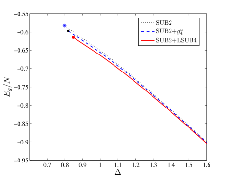
Figure 2: The ground state-energy per spin as a function of $\Delta$ for spin-1/2 XXZ model in the full SUB2, SUB2+$g_{4}^{a}$ and SUB2+LSUB4 schemes. The critical terminating points for each scheme are also indicated.

Table 1: The ground-state energy per spin for the 2D spin-1/2 XXZ model in the SUB2+LSUB4 scheme for some values of $\Delta$, together with that of the full SUB2, SUB2+$g_{4}^{a}$, and LSUB4 schemes [11].

$\Delta$	0.89	1	2	3	4	5
SUB2	-0.6118	-0.6508	-1.0807	-1.5547	-2.0413	-2.5331
SUB2+$g_{4}^{a}$	-0.6189	-0.6561	-1.0816	-1.5550	-2.0414	-2.5332
LSUB4	-0.6162	-0.6636	-1.0831	-1.5555	-2.0418	-2.5333
SUB2+LSUB4	-0.6289	-0.6641	-1.0832	-1.5555	-2.0416	-2.5333

3 Staggered Magnetization

The staggered magnetization for a general spin quantum number $s$ can be defined as,

$$M=-\frac{1}{Ns}\langle\tilde{\Psi}|\sum_{l}^{N}s_{l}^{z}|\Psi\rangle,$$ (30)

where $l$ runs over all the lattice sites for our rotated Hamiltonian of Eq. (2).

In the SUB2+LSUB4 scheme we obtain,

$$M=1-2\sum_{r}\tilde{b}_{r}b_{r}-2(\tilde{g}_{4}^{a}g_{4}^{a}+\tilde{g}_{4}^{b}g_{4}^{b}+\tilde{g}_{4}^{c}g_{4}^{c}+\tilde{g}_{4}^{d}g_{4}^{d}),$$ (31)

where two-body and four-body bra-state coefficients $\tilde{b}_{r}$ and $\tilde{g}_{4}$ are determined by the second variational Eqs. (11). We solve these equations for the bra-state in similar fashion as for the ket-state, namely by Fourier transformation for the two-body coefficients and by iteration methods for the four-body coefficients. We leave the details to Appendix and show the results in Fig. 3. We find that at the critical $\Delta_{c}$, $M_{c}=0.649$ in our SUB2+LSUB4 scheme, compared with $M_{c}=0.663$ in the SUB2+$g_{4}^{a}$ scheme and $M_{c}=0.682$ in the SUB2 obtained earlier [11]. Our SUB2+LSUB4 result is in good agreement with $M=0.6138$ of the 3rd-order spin-wave results [21], $M=0.614$ of the series expansion calculations [22], $M=0.615$ of the quantum Monte Carlo calculations [23] at $\Delta_{c}=1$. The highe-order LSUB$m$ scheme with $m$=8 produces $M=0.705$ at $\Delta=1$ before extrapolation and $M=0.616$ after an extrapolation has been made [16]. The corresponding values of $M$ at $\Delta=1$ are 0.712 in DSUB$11$ scheme [19] and 0.708 in LPSUB$6$ scheme [20].

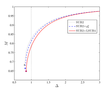
Figure 3: The staggered magnetization for the 2D spin-1/2 XXZ model for the full SUB2, SUB2+$g_{4}^{a}$ and SUB2+LSUB4 schemes.

4 Spin-wave excitation spectra

The excited state in CCM is given by applying an excitation operator $X^{e}$ to the ket-state wave function,

$$|\Psi_{e}\rangle=X^{e}|\Psi_{g}\rangle=X^{e}e^{S}|\Phi\rangle,$$ (32)

where $X^{e}$ in general is written in terms of the configurational creation operators $C_{I}^{+}$ only as,

$$X^{e}=\sum_{I}\chi_{I}^{e}C_{I}^{\dagger},$$ (33)

with the excitation coefficient $\chi_{I}^{e}$. From the Schrödinger equation $H|\Psi_{e}\rangle=E_{e}|\Psi_{e}\rangle,$ it is straightforward to derive the following equation for the excitation coefficient,

$$\varepsilon_{e}\chi_{I}^{e}=\langle\Phi|C_{I}e^{-S}[H,X^{e}]e^{S}|\Phi\rangle,$$ (34)

where $\varepsilon_{e}\equiv E_{e}-E_{g}$ is the excitation energy. Here, we consider the spin-wave excitations by including only a single spin-flip operator, $C_{I}^{\dagger}\simeq s_{i}^{+},$ similar to the SUB2 scheme as before [11]. After Fourier transform we obtain the energy spectrum in this linear approximation as,

$$\varepsilon_{e}=\varepsilon(\textbf{q})=\frac{1}{2}zKE(\textbf{q}),$$ (35)

where $K$ and $E(\textbf{q})$ are as defined before in Eqs. (23) and (24), and $z$ is the coordination number. We present the excitation gap, $\varepsilon(\textbf{q})$ at $\textbf{q}=0$, as a function of $\Delta$ in Fig. 4. As can be seen from the figure, the energy gap in the SUB2+LSUB4 scheme is smaller than that of the SUB2 and SUB2+$g_{4}^{a}$ schemes, implying that the energy gap is reduced in the higher-order approximations. For all these three schemes, the energy gap disappears at their corresponding critical anisotropy $\Delta_{c}$. It is interesting to compare our results for the energy gap with that of the high-order LSUB$m$ scheme [16]. At $\Delta=1$ our SUB2+LSUB4 gap value is $\varepsilon(0)=1.05$ while the LSUB4 and LSUB8 values are much lower at $\varepsilon(0)=0.851$ and 0.473 respectively. By employing an extrapolation, the LSUB$m$ scheme produces an energy gap close to zero, corresponding to the SUB2+LSUB4 result at the critical $\Delta_{c}$. The much lower energy gap values away from the critical region by the higher-order LSUB$m$ scheme are clearly due to the inclusion of the higher-order correlations in the excitation operators whereas we only include the linear excitation operators in our calculations as given by Eq. (33) with $C_{I}^{\dagger}\simeq s_{i}^{+}$. However, our SUB2+LSUB4 scheme has an advantage of capable of producing the full energy spectra due to inclusion of the long-range two-body correlations as discussed below.

In Fig. 5, we present our SUB2+LSUB4 results for the spin-wave energy spectrum of Eq. (35) at $\Delta_{c}$ together with that of the SUB2 results [11], and at $\Delta=1$, the results of the linear spin-wave theory (LSWT), the series expansion calculations (SE) [24], and quantum Monte Carlo calculations (QMC) [25]. The spin-wave velocity correction factor to the linear spin-wave theory in our SUB2+LSUB4 scheme is given by $K_{c}=1.23$, in good agreement with $1.18\pm 0.02$ from the series expansion and $1.21\pm 0.03$ from the quantum Monte Carlo calculations.

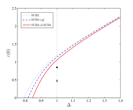
Figure 4: The excitation energy gap $\varepsilon(0)$ for the 2D spin-1/2 XXZ Heisenberg model as a function of $\Delta$, for the full SUB2, SUB2+$g_{4}^{a}$ and SUB2+LSUB4 schemes. The two gap values at $\Delta=1$ are given by the LSUB4 scheme ($\bullet$) and LSUB8 scheme ($\diamond$) of Ref. [16] where the high-order excitation correlations are included as discussed in the text.

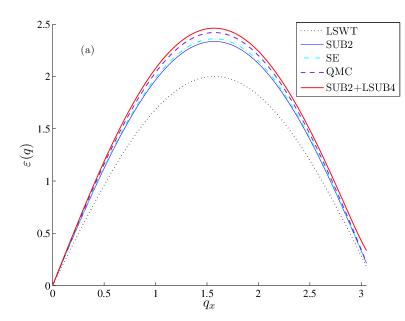
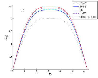
Figure 5: The spin-wave excitation spectra for the 2D spin-1/2 XXZ Heisenberg model at $\Delta_{c}$ for the CCM (SUB2 and SUB2+LSUB4) results, and at $\Delta=1$ for the linear spin-wave theory (LSWT), the series expansion (SE) [24], and quantum Monte Carlo calculations [25]. The energy spectra in (a) are for $q_{x}=q_{y}$ and those in (b) are for $q_{y}=0$.

5 Summary and Conclusion

In summary, we have obtained here numerical results for the ground-state energy, sublattice magnetization, and excitation energy for the spin-half square-lattice antiferromagnetic XXZ model using the SUB2+ LSUB4 scheme of CCM. We find that our results for the ground-state properties in general are improved when compared with those obtained by the SUB2 or LSUB4 scheme alone. In particular, due to inclusion of the two-body long-range-order correlations, the SUB2+LSUB4 scheme is capable of producing improved results around the critical regions of the anisotropy, the excitation gaps at $\textbf{q}=0$, and the full spin-wave energy spectra. Good agreement for the spin-wave spectra is found with the high-order series expansion and the quantum Monte Carlo calculations. This is contrast to the recent state-of-the-art calculations of the LSUB$m$ scheme using computer algebra, where good results of the critical properties have been obtained after an extrapolation in the limit $m\rightarrow\infty$ is made [16, 17, 18, 19, 20]. Away from the critical points, the long-range correlations are less important and the high-order LSUB$m$ clearly provides better numerical results due to inclusion of the high-order local correlations. We believe that the different approximation schemes in CCM complement each other for a more complete description of the physics of the spin-lattice Hamiltonian model, and in particular the SUB2+LSUB$m$ scheme as presented here has the advantage of producing the full excitation energy spectrum. Further improvement for the excitation energies away from the critical points can be obtained by including the higher-order local correlations in the excitations operator $X^{e}$ as demonstrated in the LSUB$m$ scheme of Ref. [16]. It will be interesting to apply our SUB2+LSUB$m$ scheme to other models such as the spin-1/2 XY model.

Acknowledgments

We are grateful to Prof. R. F. Bishop and Dr. D. J. J. Farnell for useful discussion and assistance. M. Merdan is also grateful to C. Fullerton, R. Morris, A. Bladon, A. Black and J. Challenger for their help and support.

Appendix

The ground bra-state in the SUB2+LSUB4 scheme

Similar to the ket-state equations, the bra state in the SUB2+LSUB4 scheme retains the two- and four-body bra-state correlation coefficients defined as $\tilde{b}_{r}$, and $\tilde{g}_{4}^{a}$, $\tilde{g}_{4}^{b}$, $\tilde{g}_{4}^{c}$ and $\tilde{g}_{4}^{d}$ respectively. From Eq. (11), there also are two sets of equation for the bra-state coefficients. The first set is obtained by taking the partial derivatives of the Hamiltonian expectation $\bar{H}$ with respect to $b_{r}$, thus,

$$\frac{\partial\bar{H}}{\partial b_{r}}=\sum_{\rho} \Big{[}(1+a_{1}+2(\Delta+2b_{1})\tilde{b}_{1}-4\sum_{r^{\prime}}\tilde{b}_{r^{\prime}}b_{r^{\prime}})\delta_{r,\rho}$$

$$+a_{3}^{a}\delta_{r,\rho_{3a}}+a_{3}^{b}\delta_{r,\rho_{3b}}+a_{5}^{a}\delta_{r,\rho_{5a}}+a_{5}^{b}\delta_{r,\rho_{5b}}$$

$$+a_{5}^{c}\delta_{r,\rho_{5c}}-2(\Delta+2b_{1})\tilde{b}_{r}+2\sum_{r^{\prime}}\tilde{b}_{r^{\prime}}b_{r-r^{\prime}-\rho}\Big{]}=0,$$ (36)

where the constants, $a_{1},a_{3}^{a},a_{3}^{b},a_{5}^{a},a_{5}^{b}$ and $a_{5}^{c}$ are given as,

$$a_{1}= \tilde{g}_{4}^{b}(-2\Delta b_{1}-2\Delta b_{3}^{a}+2({b_{3}^{a}})^{2}+8b_{1}b_{3}^{b}+4b_{3}^{a}b_{3}^{b}+8g_{4}^{b})+\tilde{g}_{4}^{a}(-8\Delta b_{1}$$

$$+16b_{1}b_{3}^{b}+8g_{4}^{a}+4g_{4}^{c})+\tilde{g}_{4}^{c}(-2\Delta b_{1}+6b_{1}^{2}-2\Delta b_{3}^{b}+8b_{1}b_{3}^{b}$$

$$+4({b_{3}^{b}})^{2}+g_{4}^{a}+8g_{4}^{c}+2g_{4}^{d})+\tilde{g}_{4}^{d}(-2\Delta b_{1}+3b_{1}^{2}+2b_{1}b_{3}^{a}$$

$$-2\Delta b_{3}^{b}+6b_{1}b_{3}^{b}+b_{3}^{a}b_{3}^{b}+4({b_{3}^{b}})^{2}+g_{4}^{c}+8g_{4}^{d}),$$ (37)

$$a_{3}^{a}= -4\tilde{g}_{4}^{a}g_{4}^{c}+\frac{1}{2}\tilde{g}_{4}^{d}(2b_{1}^{2}+2b_{1}b_{3}^{b}-g_{4}^{b}-g_{4}^{c}-2g_{4}^{d})-\tilde{g}_{4}^{c}(g_{4}^{a}+g_{4}^{d})$$

$$+\tilde{g}_{4}^{b}(-2\Delta b_{1}+4b_{1}b_{3}^{a}+4b_{1}b_{3}^{b}+g_{4}^{b}+2g_{4}^{d}),$$ (38)

$$a_{3}^{b}= \tilde{g}_{4}^{a}(8b_{1}^{2}-8g_{4}^{c}-8g_{4}^{d})+\tilde{g}_{4}^{b}(4b_{1}^{2}+4b_{1}b_{3}^{a}-6g_{4}^{d})+\tilde{g}_{4}^{c}(-2\Delta b_{1}+4b_{1}^{2}$$

$$+8b_{1}b_{3}^{b}-3g_{4}^{d})+\frac{1}{2}\tilde{g}_{4}^{d}(-4\Delta b_{1}+6b_{1}^{2}+2b_{1}b_{3}^{a}+16b_{1}b_{3}^{b}$$

$$-g_{4}^{b}-3g_{4}^{c}-2g_{4}^{d}),$$ (39)

$$a_{5}^{a}= -\tilde{g}_{4}^{b}\,g_{4}^{b},$$ (40)

$$a_{5}^{b}= -\frac{1}{2}\,\tilde{g}_{4}^{d}\,(g_{4}^{b}+g_{4}^{c})-\tilde{g}_{4}^{b}(2g_{4}^{b}+2g_{4}^{d})-\tilde{g}_{4}^{c}g_{4}^{d},$$ (41)

$$a_{5}^{c}= -\frac{1}{2}\,\tilde{g}_{4}^{d}\,(g_{4}^{b}+g_{4}^{c}+4g_{4}^{d})-\tilde{g}_{4}^{c}(2g_{4}^{c}+g_{4}^{d})-2\tilde{g}_{4}^{b}g_{4}^{d}.$$ (42)

and where the 2D vectors $\rho_{5a}=(5\rho_{x},0)$, $\rho_{5b}=(4\rho_{x},\rho_{y})$ and $\rho_{5c}=(3\rho_{x},2\rho_{y})$ with the nearest-neighbor vector index $\rho=(\rho_{x},\rho_{y})$.

The second set of equations for the bra-state are obtained by taking the partial derivatives for $\bar{H}$ with respect to the four-body ket-state coefficients, hence,

$$\frac{\partial\bar{H}}{\partial g_{4}^{a}}=2\tilde{b}_{1}+\tilde{g}_{4}^{a}(4\Delta+8b_{1})+\tilde{g}_{4}^{c}(b_{1}-b_{3}^{a})=0,$$ (43)

$$\frac{\partial\bar{H}}{\partial g_{4}^{b}}=2\tilde{b}_{1}+\tilde{b}_{3}^{a}+\tilde{g}_{4}^{b}(-b_{5}^{a}-2b_{5}^{b}+5\Delta+8b_{1}+b_{3}^{a})-\frac{1}{2}\,\tilde{g}_{4}^{d}\,(b_{5}^{b}$$

$$\quad\quad\quad\quad\quad\quad\quad\quad\quad\quad\quad\quad\quad\quad\quad\quad\quad\quad\quad\quad\quad+b_{5}^{c}+b_{3}^{a}+b_{3}^{b})=0,$$ (44)

$$\frac{\partial\bar{H}}{\partial g_{4}^{c}}=4\tilde{b}_{1}+\tilde{b}_{3}^{b}+\tilde{g}_{4}^{c}(-2b_{5}^{c}+5\Delta+8b_{1})+\tilde{g}_{4}^{a}(4b_{1}-4b_{3}^{a}-8b_{3}^{b})$$

$$\quad\quad\quad\quad\quad\quad\quad\quad\quad\quad\quad\quad\quad\,\,\,+\frac{1}{2}\,\tilde{g}_{4}^{d}\,(2b_{1}-b_{5}^{b}-b_{5}^{c}-b_{3}^{a}-3b_{3}^{b})=0,$$ (45)

$$\frac{\partial\bar{H}}{\partial g_{4}^{d}}=8\tilde{b}_{1}+2\tilde{b}_{3}^{b}+\tilde{g}_{4}^{b}(-2b_{5}^{b}-2b_{5}^{c}+2b_{3}^{a}-6b_{3}^{b})+\tilde{g}_{4}^{c}(-b_{5}^{b}-b_{5}^{c}$$

$$\quad\quad+2b_{1}-b_{3}^{a}-3b_{3}^{b})+\tilde{g}_{4}^{d}(-2b_{5}^{c}+5\Delta+8b_{1}-b_{3}^{a}-b_{3}^{b})-8\tilde{g}_{4}^{a}b_{3}^{b}=0.$$ (46)

Similar to the solution of the ket-state coefficients, in order to find the bra-state correlation coefficients, we obtain Fourier transformation of Eq. (Appendix The ground bra-state in the SUB2+LSUB4 scheme) which is solved together with Eqs. (43)-(46) self-consistently. We rewrite Eq. (Appendix The ground bra-state in the SUB2+LSUB4 scheme) in the following simpler form as,

$$\sum_{\rho} \Big{[}(1+a_{1}+2K\tilde{b}_{1}-4\Xi)\delta_{r,\rho}+a_{3}^{a}\delta_{r,\rho_{3a}}+a_{3}^{b}\delta_{r,\rho_{3b}}+a_{5}^{a}\delta_{r,\rho_{5a}}$$

$$+a_{5}^{b}\delta_{r,\rho_{5b}}+a_{5}^{c}\delta_{r,\rho_{5c}}-2K\tilde{b}_{r}+2\sum_{r^{\prime}}\tilde{b}_{r^{\prime}}b_{r-r^{\prime}-\rho}\Big{]}=0,$$ (47)

where $K$ is again defined in Eq. (23) and the constant $\Xi$ is given by,

$$\Xi=\sum_{r^{\prime}}\tilde{b}_{r^{\prime}}b_{r^{\prime}}.$$ (48)

After Fourier transformation, Eq. (Appendix The ground bra-state in the SUB2+LSUB4 scheme) reduces to

$$(1+a_{1}+2K\tilde{b}_{1}-4\Xi)\gamma(\textbf{q})+A(\textbf{q})-2K\tilde{\Gamma}(\textbf{q})+2\gamma(\textbf{q})\tilde{\Gamma}(\textbf{q})\Gamma(\textbf{q})=0,$$ (49)

where $\Gamma(\textbf{q})$ and $\tilde{\Gamma}(\textbf{q})$ are the Fourier transformations of the ket- and bra-state coefficients respectively, and the function $A(\textbf{q})$ is given by,

$$A(\textbf{q})= a_{3}^{a}\gamma_{3a}(\textbf{q})+a_{3}^{b}\gamma_{3b}(\textbf{q})+a_{5}^{a}\gamma_{5a}(\textbf{q})+a_{5}^{b}\gamma_{5b}(\textbf{q})+a_{5}^{c}\gamma_{5c}(\textbf{q}),$$

with $\gamma_{3a}(\textbf{q})$ and $\gamma_{3b}(\textbf{q})$ as given before in Eqs. (26) and (27) and new functions defined as,

$$\gamma_{5a}(\textbf{q})=\frac{1}{2}(\cos 5q_{x}+1),$$

$$\gamma_{5b}(\textbf{q})=\frac{1}{2}(\cos 4q_{x}+\cos q_{y}),$$

$$\gamma_{5c}(\textbf{q})=\frac{1}{2}(\cos 3q_{x}+\cos 2q_{y}).$$

Using the solution for $\Gamma(\textbf{q})$ of Eq. (22) with the definition for $E(\textbf{q})$ in Eq. (24), the physical solution of Eq. (49) for the bra-state is,

$$\tilde{\Gamma}(\textbf{q})=\frac{D\gamma(\textbf{q})+2A(\textbf{q})}{4K{E(\textbf{q})}},$$ (50)

where the constant $D$ is defined as,

$$D=2(1+a_{1}+2K\tilde{b}_{1}-4\Xi).$$ (51)

The value of $D$ can be determined self-consistently as follows. We first rewrite Eq. (48) as an integral in Fourier space as,

$$\Xi=\frac{1}{\pi^{2}}\int_{0}^{\pi}\frac{1}{4}\Big{[}D+\frac{2A(\textbf{q})}{\gamma(\textbf{q})}\Big{]}\Big{[}\frac{1}{{E(\textbf{q})}}-1\Big{]}d\textbf{{q}}.$$ (52)

The bra-state coefficient $\tilde{b}_{r}$ is obtained by inverse Fourier transformation of $\tilde{\Gamma}(\textbf{q})$,

$$\tilde{b}_{r}=\frac{1}{\pi^{2}}\int_{0}^{\pi}e^{-ir.\textbf{q}}\,\frac{D\gamma(\textbf{q})+2A(\textbf{q})}{4KE(\textbf{q})}d\textbf{q},$$ (53)

and in particular, $\tilde{b}_{1}$ is given by,

$$\tilde{b}_{1}=\frac{1}{\pi^{2}}\int_{0}^{\pi}\frac{D\gamma^{2}(\textbf{q})+2A(\textbf{q})\gamma(\textbf{q})}{4K{E(\textbf{q})}}d\textbf{{q}}.$$ (54)

Combining Eqs. (51),(52) and (54), we obtain the following expression for $D$,

$$D^{-1}=\frac{1}{c}\,\Big{[}\frac{1}{\pi^{2}}\int_{0}^{\pi}\frac{1-\gamma^{2}(\textbf{q})/2}{{E(\textbf{q})}}\,d\textbf{{q}}-\frac{1}{2}\Big{]},$$ (55)

where the constant $c$ is given by,

$$c=I+a_{1}+1,$$

with the integral $I$ defined as,

$$I=\frac{1}{\pi^{2}}\int_{0}^{\pi}\Big{[}\frac{A(\textbf{q})\gamma(\textbf{q})-2A(\textbf{q})/\gamma(\textbf{q})}{{E(\textbf{q})}}+\frac{2A(\textbf{q})}{\gamma(\textbf{q})}\Big{]}d\textbf{{q}}.$$ (56)

Using the above self-consistency equations for $\tilde{b}_{1}$, $\tilde{b}_{3}^{a}$, $\tilde{b}_{3}^{b}$, $D$ and $\Xi$ and by iteration method, we obtain the numerical values for $\tilde{g}_{4}^{a}$, $\tilde{g}_{4}^{b}$, $\tilde{g}_{4}^{c}$ and $\tilde{g}_{4}^{d}$ of the four-body bra-state coefficients. The staggered magnetization is then calculated by using Eq. (31).

References

- [1] F. Coester, Nuclear Physics 7, 421 (1958).
- [2] J. Čížek, The Journal of Chemical Physics 45, 4256 (1966).
- [3] J. Paldus, J. Čížek, and I. Shavitt, Phys. Rev. A 5, 50 (1972).
- [4] H. Kümmel, K. Lührmann, and J. Zabolitzky, Physics Reports 36, 1 (1978).
- [5] R. Bishop and K. Lührmann, Phys. Rev. B 17, 3757 (1978).
- [6] J. Arponen, Annals of Physics 151, 311 (1983).
- [7] J. Arponen, R. Bishop, and E. Pajanne, Phys. Rev. A 36, 2539 (1987).
- [8] R. J. Bartlett, The Journal of Physical Chemistry 93, 1697 (1989).
- [9] R. F. Bishop, Theoretica Chimica Acta 80, 95 (1991).
- [10] M. Roger and J. Hetherington, Phys. Rev. B 41, 200 (1990).
- [11] R. F. Bishop, J. B. Parkinson, and Yang Xian, Phys. Rev. B 44, 9425 (1991).
- [12] R. Bursill et al., Journal of Physics: Condensed Matter 7, 8605 (1995).
- [13] R. Bishop, R. Hale, and Y. Xian, Phys. Rev. Letters 73, 3157 (1994).
- [14] D. J. J. Farnell, S. E. Krüger, and J. B. Parkinson, Journal of Physics: Condensed Matter 9, 7601 (1997).
- [15] R. Bishop, D. Farnell, and J. Parkinson, Phys. Rev. B 58, 6394 (1998).
- [16] R. F. Bishop et al., Journal of Physics: Condensed Matter 12, 6887 (2000).
- [17] D. Farnell, K. Gernoth, and R. Bishop, Phys. Rev. B 64, 172409 (2001).
- [18] R. F. Bishop, P. Li, D. J. J. Farnell, and C. E. Campbell, Phys. Rev. B 79, 174405 (2009).
- [19] R. Bishop, P. Li and J. Schulenburg, Journal of Physics: Condensed Matter 12, 479 (2009).
- [20] R. Bishop and P. Li, Phys. Rev. A 83, 042111 (2011).
- [21] C. Hamer and P. Arndt, Phys. Rev. B 46, 6276 (1992).
- [22] Z. W. Oitmaa J and C. J. Hamer, Phys. Rev. B 43, 8321 (1991).
- [23] K. Runge, Phys. Rev. B 45, 12292 (1992).
- [24] R. Singh, Phys. Rev. B 39, 9760 (1989).
- [25] G. Chen, H.-Q. Ding, and W. Goddard, Phys. Rev. B 46, 2933 (1992).