Maximum-likelihood reconstruction of photon returns from simultaneous analog and photon-counting lidar measurements

Abstract

We present a novel method for combining the analog and photon-counting measurements of lidar transient recorders into reconstructed photon returns. The method takes into account the statistical properties of the two measurement modes and estimates the most likely number of arriving photons and the most likely values of acquisition parameters describing the two measurement modes. It extends and improves the standard combining (“gluing”) methods and does not rely on any ad hoc definitions of the overlap region nor on any background subtraction methods.

I Introduction

In order to extend the total dynamic range of measurements the same back-scattered return signal in modern lidar acquisition systems (a.k.a. transient recorders) is usually sampled with two distinct methods: a fast analog-to-digital converter and a photon counting unit eichinger . The two range-resolved traces are then combined (“glued”) by first correcting the dead-time effects of the photon counting mode donovan and then by calibrating (fitting) the analog trace to the photon counts in some suitable photon-counting rate interval gluing ; newsom ; whiteman . The final step in the construction of the “glued” trace involves choosing a suitable signal size above which only rescaled analog values are considered and below which only the photon-counting trace is used. The general usability of such “gluing” methods is hampered by several intrinsic weaknesses: the “background” is usually subtracted from both measurement modes whereas it could be retained and used as additional information; a large variety of regressions and $\chi^{2}$ minimizations are used in the calibration of the analog signal; arbitrary and not well defined photon-counting rate fitting intervals are imposed in order to stabilize the former minimizations; photon-counting nonlinearity is usually corrected only with manufacturer-supplied dead-time values licel-gluing ; the unused half of the measured data is simply discarded and the actual position of the crossover between the analog and the photon-counting trace is not selected by any strict rules.

II Measurement

This new method is based on the elementary observation that the same input signal is evaluated by two different measurement techniques. Employing simple models of these two measurement processes we will make use of all available data to construct a new composite trace of arriving photon numbers in such a way that the new hypothetical number of photons would in fact most likely produce the two actually measured traces.

For the sake of clarity we will keep the measurement models simple enough to illustrate the main properties of the method. Nevertheless, the procedure is highly flexible and if greater levels of detail are required, then the descriptions in Eq. (1)–(4) can be simply updated with more complex descriptions of the two measurement processes.

II.1 Analog signal

In a typical transient recorder, the analog signal is constructed by integrating the current from a photomultiplier (PMT) in a sampling time $\Delta t$ which is then discretized by an analog-to-digital converter into the analog lidar trace. Since the PMT is a fairly linear sensor of arrived photons $p$, we can thus describe their transformation into an analog signal $a$ with a simple linear transformation

$$a=A(p)=\alpha p+\beta,$$ (1)

where $\alpha$ is related to the PMT and amplifier gain, converting the number of incoming photons into the adc units. $\beta$ is a small hardware-imposed offset (baseline) which enables the detection of a possible signal undershoot and post-measurement determination of a true zero. Given the number of the input photons $p$, the variance, $V[a]$, of the analog signal resulting from the noise in this chain of electronics can be, at least for small signals, safely modeled as being constant,

$$V[a]=\gamma^{2}$$ (2)

and is expressed in units of $\mathrm{adc^{2}}$. For larger signals the analog variance in Eq. (2) acquires an additional signal-size dependent Poisson term which we can neglect for reasons given later.

II.2 Photon-counting mode

In typical photon-counting modules of modern transient recorders, the input photons $p$ are recorded by counters with predominantly non-extending dead-time $\tau$. These types of counters are also referred to as cumulative or non-paralyzable counters.

For such counters the mean number of counts $m$ in a sampling time $\Delta t$ can be expressed as

$$m=C(p)=\frac{p}{1+\delta p},$$ (3)

where $\delta$ is the fraction of dead-time vs. sampling time, $\delta=\tau/\Delta t$. The variance of the photon count is

$$V[m]=V_{\delta}(p),$$ (4)

where $V_{\delta}$ is a nontrivial function for the variance of the dead-time counter and is explained in greater detail in Appendix A.

Note that the dead time, during which the counter is unable to record any incoming photons, induces saturation of the maximally possible counts to $m_{\text{max}}\approx\lim_{p\to\infty}C(p)=1/\delta$. As mentioned before, the standard gluing procedure involves, before fitting the analog and photon counting traces, correcting the counts $m$ for the dead-time effects with the inverse of the function in Eq. (3),

$$p=C^{-1}(m)=\frac{m}{1-\delta m}.$$ (5)

Unfortunately, the inverse has a singularity at $m=m_{\text{max}}$ and produces negative photon estimates $p$ for $m>m_{\text{max}}$. In the standard gluing procedure this, and the fact that the dead time $\tau$ is not well known, limits the range of useful data of the measured photon counting traces.

As we will see later on, the procedure developed here does not suffer from this drawbacks since only the non-singular function $C(p)$ is used and the estimation of the dead-time value is part of the method.

II.3 Overlap region

In the case of a large number of incoming photons, $p\gg 1/\delta$, only the analog signal carries useful information due to the inevitable saturation of the photon counter. For a small photon influx the situation is reversed since the analog signal has reached the levels of the electronic noise while the photon-counting is in the ideal proportional mode with almost no dead-time effects. Therefore, outside of the relative overlap region, the quality of data of one or the other mode prevails. From the simple measurement models given above we thus require good accuracy in the overlap region and that the winning model is supplying the correct solution far away from the overlap.

Due to these relaxed requirements we can approximate the variance of the dead-time affected photon counter in Eq. (4) with the Poisson variance of the photon-count itself (see Appendix A),

$$V[m]=m=C(p).$$ (6)

II.4 Summation of lidar traces

It is quite common practice in lidar measurements to additionally increase the dynamical range of the data acquisition by summation (time stacking) of consecutive lidar returns. With fast laser-pulse repetition rates it is reasonable to assume that within the summation time the atmosphere does not introduce substantial sources of additional variance beyond the natural Poisson-like fluctuations of the backscattered photons.

Denoting by $a_{\text{s}}$ the sum of $N_{\text{s}}$ analog measurements $a$ at the same range of consecutive lidar traces and with $p_{\text{s}}$ the sum of the arrived photons, the photon conversion in Eq. (1) is transformed into $a_{\text{s}}=N_{\text{s}}A(p_{\text{s}}/N_{\text{s}})=\alpha p_{\text{s}}+N_{\text{s}}\beta$. The variance in Eq. (2) scales as $V[a_{\text{s}}]=N_{\text{s}}\gamma^{2}$.

The mean photon count obtained by summation of $N_{\text{s}}$ consecutive lidar returns, $N_{\text{s}}C(p_{\text{s}}/N_{\text{s}})$, has a nice property of retaining the general form of Eq. (3) with the dead-time fraction effectively transformed into $\delta/N_{\text{s}}$. Nevertheless, for large photon numbers $p$ the variance depends on summation in a non-linear way and has to be evaluated as $N_{\text{s}}V_{\delta}(p_{\text{s}}/N_{\text{s}})$.

The measurement models given above are thus, at least to some degree, invariant with respect to the summation as long as the following transformation of the acquisition parameters is taken into account,

$$\alpha\mapsto\alpha,\quad\beta\mapsto\beta/N_{\text{s}},\quad\gamma^{2}\mapsto\gamma^{2}/N_{\text{s}},\quad\delta\mapsto N_{\text{s}}\delta.$$ (7)

III Initial estimates

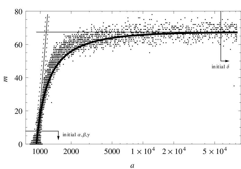
Figure 1: Plot of analog vs. photon-counting data points $(a_{i},m_{i})$ for $N_{\text{s}}=20$ summed lidar returns. The slanted line on the left is a fit for the photon-to-analog conversion parameters $\alpha$, $\beta$ and $\gamma^{2}$ in the range of the lower left corner (indicated by the left arrow-box) with dashed lines illustrating variance $a\pm 2\gamma$. The horizontal line is a fit for dead-time fraction $\delta$ in the range of the upper right corner (right arrow-box). The thick line is the resulting prediction for $m=C(A^{-1}(a))$.

For any nonlinear minimization procedure it is of utmost importance to acquire accurate initial values for minimized parameters. In our case the initial values for parameters $\alpha$, $\beta$, $\gamma^{2}$ are obtained from a least-squares minimization of

$$\chi^{2}_{\text{min}}=\min_{\alpha,\beta}\sum_{i}[a_{i}-A(m_{i})]^{2},$$ (8)

where only analog and photon-counting data points $(a_{i},m_{i})$ of the lower left corner are used (see Fig. 1), i.e. the lower 10% of the whole photon-count range. Initial estimates for the “gluing” parameters $\alpha$ and $\beta$ are thus obtained in a manner similar to the standard procedure suggested by the manufacturers of the transient recorders licel-gluing or other more detailed studies whiteman .

Since the fluctuations of the analog data in the lower left corner of Fig. 1 are dominated by the electronic noise, an estimate for the analog variance $\gamma^{2}$ is obtained simply from the residuals in Eq. (8), $\gamma^{2}=\chi^{2}_{\text{min}}/N_{\text{dof}}$, where the number of degrees of freedom is $N_{\text{dof}}=N-2$ with $N$ the number of data points involved in the fit. From this point on, $\gamma^{2}$ is kept fixed and will not be the subject of minimization.

Fitting the photon counts $m$ to a constant in the tail of the large analog values (upper right corner of Fig. 1) gives an estimate for the dead-time fraction, $\delta=1/\langle m\rangle$. For the $\langle m\rangle$ estimate typically only the data in the largest 30% of the analog values has been used, but excluding all data points with ADC saturation (which we discard in this procedure anyway).

See Fig. 1 for the results of the initial fits to an example lidar return which will be used throughout this analysis. The data was obtained with a back-scatter lidar at wavelength of 355 nm, pulse repetition rate of 20 Hz and trace summation $N_{\text{s}}=20$. The light sensor was a Hammamatsu R3200 photomultiplier tube connected to a high-voltage of approximately 800 V. The return signal was acquired with a Licel TR 40-160 transient recorder operated at a sampling frequency of 40 MHz. The recorder is delivering discretized analog signal traces with 12 bit ADC resolution and photon-counting traces with a maximal count rate of 250 MHz, both with trace depth of 16k samples licel . The example trace was recorded with $20^{\circ}$ elevation on a relatively clear night and contains only a thin and faint layer of haze around the range of 13.5 km.

IV Maximum likelihood

From the two measurement models described above we can construct a likelihood $\mathcal{L}$ for the total trace as a product over all trace time elements $i$ of a likelihood of observing $p_{i}$ photons given the analog measurement $a_{i}$ and the photon count $m_{i}$,

$$\mathcal{L}=\prod_{i}\mathcal{L}(a_{i},m_{i},p_{i}),$$ (9)

where likelihood $\mathcal{L}(a_{i},m_{i},p_{i})$ is a product of the probability $P(a_{i}|p_{i})$ to observe an analog signal and the probability to have a certain photon count $P(m_{i}|p_{i})$ given a number of photons. We can model the analog probability with the normal (Gauss) distribution $\mathcal{N}(x,\sigma^{2})=\exp(-x^{2}/2\sigma^{2})/\sqrt{2\pi\sigma^{2}}$ using the linear transformation Eq. (1) and the corresponding variance $\gamma^{2}$. According to Eq. (6), the photon count probability can be approximated with the Poisson distribution from Eq. (26) so that the resulting likelihood is expressed as

$$\mathcal{L}(a_{i},m_{i},p_{i})=\mathcal{N}(a_{i}-A(p_{i}),\gamma^{2})\times\mathcal{P}_{m_{i}}(C(p_{i}))$$ (10)

The corresponding deviance is defined as

$$\mathcal{D} =-2\ln\mathcal{L}=-2\sum_{i}\ln\mathcal{L}(a_{i},m_{i},p_{i})=$$

$$=\sum_{i}\mathcal{D}(a_{i},m_{i},p_{i}),$$ (11)

where

$$\mathcal{D}(a_{i},m_{i},p_{i}) =\ln 2\pi\gamma^{2}+\frac{[a_{i}-A(p_{i})]^{2}}{\gamma^{2}}\,+$$

$$+2\left[\ln m_{i}!+C(p_{i})-m_{i}\ln C(p_{i})\right]$$ (12)

is the deviance for a particular data point. The motivation for using the deviance version of likelihood comes from the fact that for the normal-like distribution probabilities the deviance is equivalent to the usual $\chi^{2}$ estimator. Nevertheless, the minimization of Poisson-like distribution probabilities can not be formulated in terms of a simple $\chi^{2}$ formalism.

The solution to the minimal deviance (or, in other words, maximal likelihood)

$$\mathcal{D}=\text{min}.$$ (13)

is usually found by solving for an extreme

$$\nabla\mathcal{D}\equiv 0,$$ (14)

where the gradient $\nabla$ is formed by derivatives over the whole parameter space. In our two-measurement model, the deviance (likelihood) depends on the following parameters: the $\alpha$ and $\beta$ coefficients from the analog-to-digital conversion $A(p)$, the variance of the analog signal $\gamma^{2}$, and the dead-time fraction $\delta$ of the photon counter. In addition to these four model parameters, the deviance depends also on all (unknown) numbers of incoming photons $p_{i}$. In general, the deviance thus has $N+4$ parameters for $2N$ data points (analog and photon counts).

Due to the particular structure of the deviance in Eq. (11), we can split the global minimization procedure for $\mathcal{D}$ in two parts: the outer part drives the minimization over $\alpha$, $\beta$, $\gamma^{2}$ and $\delta$ parameters, and the inner part deals with the “nuisance” parameters $p_{i}$ for each iteration of the outer part.

Assuming that the outer part already supplies parameters $\alpha$, $\beta$, $\gamma^{2}$ and $\delta$, the inner part proceeds as follows: since in the total deviance $\mathcal{D}$ only the $i$th term $\mathcal{D}(a_{i},m_{i},p_{i})$ depends on particular $p_{i}$, we can simplify the $p_{i}$ part of its gradient,

$$\frac{\partial\mathcal{D}}{\partial p_{i}}=\frac{\partial\mathcal{D}(a_{i},m_{i},p_{i})}{\partial p_{i}},$$ (15)

by introducing a marginalized (conditional) number of photons,

$$\tilde{p}_{i}=\operatorname*{arg\,min}_{p_{i}}\mathcal{D}(a_{i},m_{i},p_{i}),$$ (16)

and profile deviance (as in profile likelihood)

$$\hat{\mathcal{D}}(a_{i},m_{i})=\min_{p_{i}}\mathcal{D}(a_{i},m_{i},p_{i})=\mathcal{D}(a_{i},m_{i},\tilde{p}_{i}).$$ (17)

Solving this equation for all $p_{i}$ produces a total deviance without the nuisance parameters $p_{i}$. Finally, the deviance is contracted into

$$\hat{\mathcal{D}}=\sum_{i}\hat{\mathcal{D}}(a_{i},m_{i}),$$ (18)

which depends only on the remaining four parameters $\alpha$, $\beta$, $\gamma^{2}$, and $\delta$, and is minimized by the outer part of the procedure.

For our two particular measurement models, Eqs. (15)–(17) in the inner part of the minimization correspond to finding a suitable root of a polynomial of the fourth order in $p_{i}$. Although analytical solutions exist, they are not very practical for real application. The solution can be obtained with the Newton-Raphson iteration

$$\tilde{p}_{i}^{[j+1]}=\tilde{p}_{i}^{[j]}-\frac{\mathcal{D}^{\prime}(a_{i},m_{i},\tilde{p}_{i}^{[j]})}{\mathcal{D}^{\prime\prime}(a_{i},m_{i},\tilde{p}_{i}^{[j]})}$$ (19)

where $\mathcal{D}^{\prime}$ and $\mathcal{D}^{\prime\prime}$ are respectively the first and the second derivative of $\mathcal{D}(a_{i},m_{i},p_{i})$ with respect to $p_{i}$ in Eq. (12). The iteration in Eq. (19) is started with a suitable approximation $\tilde{p}_{i}^{[0]}$ and is repeated until $\left|\tilde{p}_{i}^{[j+1]}-\tilde{p}_{i}^{[j]}\right|$ becomes smaller than $\varepsilon$, with $\varepsilon$ set to some small number ($\sim 10^{-6}$). Note that in some cases the minimum over $p_{i}$ is not the zero of the derivative in Eq. (15), but can be instead found at the boundary, $p_{i}=0$, of the validity interval of the $p_{i}$ parameter.

The outer part of the minimization deals with the total deviance in Eq. (18) with respect to the remaining non-fixed parameters and this can be carried out with a variety of nonlinear minimization procedures (see for example minuit ). Denoting the final values of the parameters in the deviance minimum with $\tilde{\alpha}$, $\tilde{\beta}$, and $\tilde{\delta}$, the set of final values of nuisance parameters

$$\breve{p}_{i}=\tilde{p}_{i}(\tilde{\alpha},\tilde{\beta},\gamma^{2},\tilde{\delta})$$ (20)

in the global minimum of the deviance represents the ultimate (most likely) synthesis of the analog and photon-counting modes of the lidar data acquisition. Note that $\gamma^{2}$ is kept fixed at the value of the initial approximation throughout this procedure.

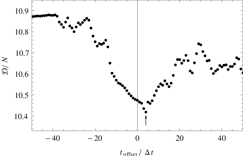
Figure 2: Dependence of the normalized deviance $\mathcal{D}/N$ on relative offset $t_{\text{offset}}$ between the analog and photon-counting traces. The arrow indicates the position of the minimum at $t_{\text{offset}}=4\Delta t=100\,\mathrm{ns}$.

IV.1 Relative acquisition delay

In the acquisition system the input signal flows through quite different electronic sub-components of the transient recorders (e.g. see schematic in manual licel ) so expecting hardware and firmware related differences in delay time is highly justified. The final analog and photon counting traces can thus be subject to substantial relative offset. In the case of our particular recorder this offset amounts to four sample times, $t_{\text{offset}}=4\,\Delta t=100\,\mathrm{ns}$. The dependence of the total deviance on $t_{\text{offset}}$ is shown in Fig. 2. How this offset is influencing the details of the example trace can be observed in Fig. 3. The two haze features found around 13.5 km in the analog and (uncorrected) photon-count modes perfectly match after the $t_{\text{offset}}$ shift. The same holds for the small noise-like features in the rest of the trace, mostly responsible for the distinct minimum of deviance in Fig. 2.

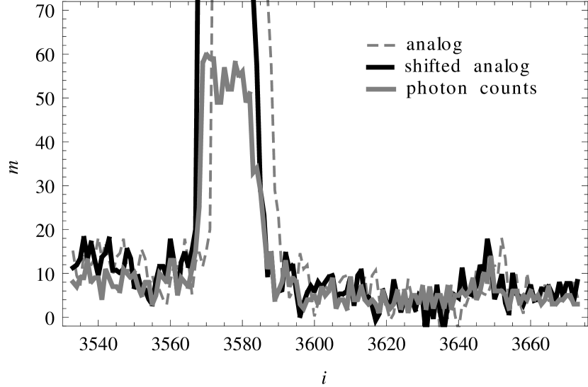
Figure 3: Haze feature before and after the shift of the analog trace. The interval $[3450,3660]$ in $i$ corresponds to $[13.275,13.725]$ km in range.

IV.2 Parameter bias due to data distribution

Typical lidar returns do not cover uniformly the whole dynamic range available in analog, $a$, and photon-counting, $m$, modes. Most of the data resides in the tail of the lidar return, occupying only the lower-left sector of the $(a,m)$ phase space (c.f. Fig. 1). The large contribution of this sector can thus introduce a bias in the likelihood maximization procedure. Furthermore, the acquisition parameters are influenced by the different parts of the $(a,m)$ phase space. Analog baseline $\beta$ is well defined by the lidar tail (lower left sector in Fig. 1), the dead-time fraction $\delta$ is mostly sensitive to the large-signal parts (upper right sector), and the photon-to-analog coefficient $\alpha$ is mostly influenced by the small and medium part of the trace (left side in Fig. 1). To remove and quantify this bias we can bin the data with several different partitions of the $(a,m)$ phase space and balance the relative contribution of each data point $(a_{i},m_{i})$ to the total deviance with a weight $w(a_{i},m_{i})=w_{j}$, where $j$ is the appropriate bin index. To maintain the correspondence with the previous non-binned case (equivalent to the binning with $w_{j}=1$) all binning variants are required to satisfy a summation rule $\sum_{j}w_{j}=N$, with $N$ being the number of data points. In all binning variants the weight should be proportional to the inverse density so that all points in a particular bin contribute to the deviance with the same weight as the other non-empty bins. With these two requirements the weights are obtained as

$$w(a_{i},m_{i})=w_{j}=\frac{N}{N_{\emptyset}N_{j}},$$ (21)

where $N_{\emptyset}$ is the number of non-empty bins and $N_{j}$ the number of data points in a particular bin $j$.

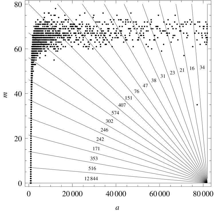
Figure 4: Example of a debiasing binning of data points $(a_{i},m_{i})$ from the example lidar return into the fan-like bins. Note that the bottom bin contains many more data points than all of the other bins. The total deviance weights are set proportionally to the inverse of the particular bin count $N_{j}$, which is also shown for all bins.

The debiased version of deviance from Eq. (18) is now written as

$$\hat{\mathcal{D}}=\sum_{i}w(a_{i},m_{i})\,\hat{\mathcal{D}}(a_{i},m_{i}).$$ (22)

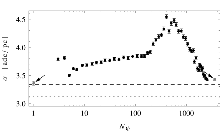
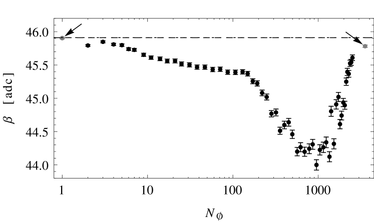
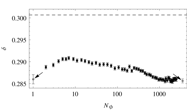
Figure 5: Dependence of the analog parameters $\alpha$, $\beta$ and photon-count parameter $\delta$ on the number of non-empty bins $N_{\emptyset}$ for the fan-like binning (black points). Left and right arrows indicate parameter values from the un-binned and the infinitely-fine binned cases, respectively. The values from the initial estimates are shown in dashed and dotted lines (see the text for more details).

Here we consider several variants of the binning divisions.

• Un-binned case, $w(a_{i},m_{i})=1$: every data point is considered with the same weight. Note that in this way in cases of lidar traces with long tails, the overwhelming contribution will come from the points with small values in both modes $a_{i}$ and $m_{i}$.

• Fan-like binning: data is categorized into a histogram with fan-like bin shapes radiating from the lower right corner, $(a_{\text{max}},m_{\text{min}})\equiv(2^{12},0)$ (see Fig. 4–left).

• Infinitely-fine binning: since both measurement modes $a_{i}$ and $m_{i}$ have only discrete integer values, we treat each of these discrete points with the same weight.

In the top two panels of Fig. 5 initial estimates for the analog parameters $\alpha$ and $\beta$ are shown for two versions of the $\chi^{2}$ fit from Eq. (8). The dashed lines are for the $\chi^{2}$ with squares of $a_{i}-A(m_{i})$ (involving uncorrected photon-counts) and the dotted lines are for a version where the dead-time fraction $\delta$ is estimated first and then the $\chi^{2}$ is constructed with dead-time corrected photon counting, $a_{i}-A(C^{-1}(m_{i}))$. In the bottom panel of Fig. 5 the initial estimate for dead time $\delta$ is shown as a dashed line. The arrows on the left and the right of all panels are indicating the results of the un-binned and the infinitely-fine binned cases, respectively. The rest of the points correspond to the fan-like binning for different granularity of the binning represented by the number of non-empty bins $N_{\emptyset}$.

While there are only minor differences between the un-binned and infinitely binned results, the fan-like binning exhibits large variations of the order of 25% for $\alpha$, 5% for $\beta$, and 15% for $\delta$ when changing the binning size. Nevertheless, with increasingly fine binning the parameters tend to converge to the two values obtained by the un-binned and infinitely binned cases, indicating that (at least for this trace depth) the maximum likelihood method is only mildly biased by the particular data distribution. On the other hand, in longer traces the distribution of the data in the lower left sector might influence the reconstruction, especially if the measurement models are not accurate enough.

V Results

V.1 Reconstructed number of photons

In order to follow the evolution of the reconstructed (most likely) number of photons $\breve{p}$ from Eq. (20) let us introduce a transition indicator

$$u=\frac{p_{m}-\breve{p}}{p_{m}-p_{a}},$$ (23)

where $p_{a}$ and $p_{m}$ are direct estimates for photons obtained from the two measurements,

$$p_{a}=A^{-1}(a)=\frac{a-\beta}{\alpha}$$ (24)

is the analog-to-photon conversion (inverse of Eq. (1)) and

$$p_{m}=C^{-1}(m)=\frac{m}{1-\delta m}$$ (25)

is the corrected photon count (inverse of Eq. (3)). Note that the latter works only for $m<1/\delta$. The values of the indicator $u$ defined in this way will be close to 1 when the reconstructed number of photons $\breve{p}$ is close to the prediction from the current inversion $p_{a}$. On the other hand, $u$ will be close to 0 when $\breve{p}$ is close to the dead-time corrected photon-count $p_{m}$. Values between 0 and 1 are indicating transition between the two measurements.

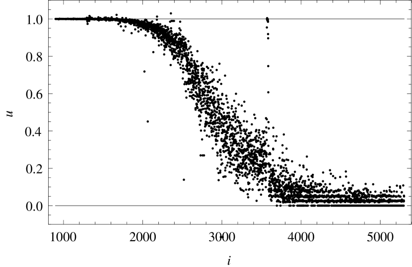
Figure 6: Behavior of the transition indicator $u$ from Eq. (23). The $[1500,5000]$ interval in $i$ corresponds to the $[5.625,18.75]$ km interval in range.

In Fig. 6 the changing of the value of indicator $u$ along our example trace is shown. We can clearly identify three regions of the indicator’s behavior.

For indices $i$ below $\sim 2000$ the indicator $u\approx 1$ and thus the reconstructed number of photons is closely following the estimate from the analog signal. In this region the photon counting is saturated and, due to the dead-time, its resolution is heavily suppressed. The maximum likelihood method thus shifts the result towards the more accurate measurement: the analog signal.

For indices $i$ above $\sim 4000$ the indicator $u\approx 0$ and the reconstructed number of photons is closely following the photon-counting. Here the analog signal is diving into the noisy region around the analog baseline where SNR is small. On the other hand, the photon counting is far from being effected by the dead-time and thus maximum likelihood gives it deserved emphasis.

In the intermediate region, for indices $i$ between $\sim 2000$ and $\sim 4000$ where $0<u<1$, the reconstructed number of photons lies between the two measurements which both have degraded accuracy, analog signal due to poor SNR and photon-counting due to the dead-time effects. Nevertheless, the value of $\breve{p}$ is chosen according to the maximum likelihood, effectively combining the two less accurate measurements into one with smaller error.

Note that all variants of the standard ”gluing” procedures would in this picture produce a step-like functional form of indicator $u$, abruptly crossing over from 1 to 0 at a position that depends on a particular choice of the “gluing” method.

V.2 Multiple lidar traces and dynamic range

Standard processing of the lidar returns usually employs extensive stacking (summation) of the lidar traces in order to increase the SNR ratio. Since the maximum likelihood method has no built-in notion of range and data-point ordering, multiple traces can instead be concatenated in order to increase the accuracy of the reconstruction. All points from different traces can thus be treated equally and processed at the same time, as long as the acquisition parameters $\alpha$, $\beta$, $\gamma^{2}$, and $\delta$ are considered stable in the respective time frame of the recording of the traces. Nevertheless, this procedure will suffer a slowdown linear with the number of data points used.

In case of our equipment, relative scatter of the reconstructed parameters within individual 480 s runs were below 1.6% for $\alpha$, 0.24% for $\beta$, and 0.28% for $\delta$. Relative differences between the mean values of the reconstructed parameters for the runs from the beginning and the end of the measurement campaign were below 0.61% for $\alpha$, 0.54% for $\beta$, 1.62% for $\gamma^{2}$, and 0.18% for $\delta$. In such stable conditions it is thus possible to concatenate a large number of lidar traces in order to increase the accuracy of the reconstructed photon returns.

In the usual lidar operation, the gain of the analog channel is set to a level which produces a discretized trace with the maximum signal slightly below (or, like in our case, above) the ADC saturation limit. In this way the analog signal can cover the whole dynamic range of the ADC, exposing nicely the saturation of the photon counting (see Fig. 1). It turns out that if for whatever reason the analog signal is covering only a smaller fraction of the available dynamic range or that the amount of photons is not saturating the photon counting, the procedure described above will still produce stable and reasonable estimates of the $\alpha$, $\beta$, and $\gamma^{2}$ parameters since they are anyway dominated by the data in the lower-left corner of the $(a_{i},m_{i})$ diagram. On the other hand, the dead-time fraction $\delta$ will in this case tend to zero (towards the ideal counter), since the absence of the photon-counting saturation in the data effectively gives an estimate $1/\delta\to\infty$, but all this without actually influencing the reconstructed number of photons $p_{i}$.

VI Discussion and conclusions

Modern transient recorders offer two principally different measurements of the same photon return: the digitization of the analog signal and the photon-counting mode. We are thus challenged, not only to use them in their respective regions of validity (like the usual “gluing” methods) but to combine them into a more accurate estimate of the photon numbers by using detailed statistical models of both acquisition processes.

The maximum likelihood procedure described in this work offers a reconstruction of photon returns that has a natural transition between the analog and photon-counting signals and is based on their analytical measurement models. In this work we have been using fairly rudimentary models of the two measurement processes, nevertheless they still adequately capture the main strengths of the new reconstruction procedure. Furthermore, if more detailed models are needed, they can be simply included into the probability expressions entering the likelihood function.

In this method we are strongly discouraged to attempt any kind of background subtraction. The background photons are treated as a normal signal since they appear in both measurement modes as viable data. Any removal of background (from dawn or daylight) should be done on the final reconstructed photon numbers.

The maximum likelihood method works in all conditions, even in the presence of clouds or other enhanced scattering objects. It fails only when the input levels of photons are not exploring the whole dynamic range of the transient recorder (i.e. both corners of Fig. 1) and thus no reliable estimate of the acquisition parameters $\alpha$, $\beta$, $\gamma^{2}$, and $\delta$ can be obtained. Through the offset analysis of the likelihood value it offers a simple way for estimation of the potential relative delay between the two measurement traces, which in our particular case turned out not to be negligible.

The code implementing the maximum-likelihood reconstruction of lidar returns is available under the GPL3 license at http:/​​/www.ung.si/~darko/lidar/.

Appendix A Dead-time counter

For an ideal counter with sampling time $\Delta t$ the discrete probability distribution of the number of counts $k$ for a Poisson process with rate $r$ and mean $M=r\Delta t$ is given by $\mathcal{P}_{k}(M)$ where

$$\mathcal{P}_{k}(x)=\frac{x^{k}e^{-x}}{k!}.$$ (26)

For a counter with non-extending dead-time $\tau$ axton the corresponding probability distribution can be found in Ref. mueller . Restructuring the equations and performing partial summations of the expressions given there, the probability $W_{k}$ of observing $k$ counts now becomes

$$W_{k}=\frac{1}{1+M\delta}\left[R_{k-1}-2R_{k}+R_{k+1}+\Delta_{k}\right],$$ (27)

where $\delta=\tau/\Delta t$, the short-hand $R_{k}=R_{k}(t_{k})$ and the truncated mean for $k$ counts is given by

$$t_{k}=M(1-k\delta).$$ (28)

$R_{k}=R_{k}(t_{k})$ is fully expressed as

$$R_{k}(x) =U(x)\sum_{j=0}^{k-1}(k-j)\mathcal{P}_{j}(x)=$$

$$=U(x)[(k-x)\,Q(k,x)+k\mathcal{P}_{k}(x)],$$ (29)

where $Q(j,x)=\Gamma(j,x)/\Gamma(j)$ is the regularized upper incomplete Gamma function walck , with the upper incomplete Gamma function

$$\Gamma(a,x)=\int_{x}^{\infty}u^{a-1}e^{-u}\,{\rm d}u$$ (30)

and $\Gamma(a)=\Gamma(a,0)$. The unitary step function $U(x)$ is defined in the usual way,

$$U(x)=\begin{cases}1&\text{if $x>0$},\\ 0&\text{otherwise},\end{cases}$$ (31)

and the remainder $\Delta_{k}$ in Eq. (27) is given explicitly as

$$\Delta_{k}=\begin{cases}0&\text{if $k\leqslant K-1$},\\ (K+1)(1+M\delta)-M&\text{if $k=K$},\\ M-K(1+M\delta)&\text{if $k=K+1$}.\end{cases}$$ (32)

The upper limit on possible counts depends on the dead-time fraction,

$$K=\lfloor 1/\delta\rfloor,$$ (33)

where $\lfloor x\rfloor$ is denoting the largest integer smaller (and not equal) than $x$.

The mean dead-time count $m$ can be expressed in terms of the ideal count $M$ as

$$m=C(M)=\frac{M}{1+M\delta}.$$ (34)

The exact expression for the variance of the dead-time counter is

$$V_{\delta}= \frac{2}{1+M\delta}\sum_{k=0}^{K}\left[(k-t_{k})\,Q(k,t_{k})+k\mathcal{P}_{k}(t_{k})\right]+$$

$$+H(m-K),$$ (35)

where the “hump” function is defined as $H(x)=x(1-x)$.

Using $d=M\delta$ as a mean “lost” count, for $d\ll 1$ the exact variance from Eq. (35) asymptotically mueller behaves as

$$V_{\delta}\approx M\left[\frac{1}{(1+d)^{3}}+\frac{\mu^{2}(6+4d+d^{2})}{6M(1+d)^{4}}\right],$$ (36)

where the part in the square brackets is the suppression factor relative to the Poisson variance $V_{\text{Poisson}}=M$. For $d\gg 1$ the variance is well described by a fully saturated dead-time counter,

$$V_{\delta}\approx H(m-K)=H(\operatorname{frac}(m)),$$ (37)

where $\operatorname{frac}(x)=x-\lfloor x\rfloor$ is the function returning fractional (non-integer) part of an argument. Note that the expression for asymptotic variance in Eq. (36) converges in this regime to 1/6 and thus well describes the average of the oscillatory dependence of $V_{\delta}$ on $\delta$ in Eqs. (35) and (37).

References

- (1) V. A. Kovalev and W. E. Eichinger, Elastic Lidar (Wiley, 2004), pp. 136–141.
- (2) D. P. Donovan, J. A. Whiteway, and A. I. Carswell, “Correction for nonlinear photon-counting effects in lidar systems”, Appl. Opt. 32, 6742–6753 (1993).
- (3) Z. Liu, Z. Li, B. Liu, and R. Li, “Analysis of saturation signal correction of the troposphere lidar”, Chin. Opt. Lett. 7, 1051–1054 (2009).
- (4) R. K. Newsom, D. D. Turner, B. Mielke, M. Clayton, R. Ferrare, and C. Sivaraman, “Simultaneous analog and photon counting detection for Raman lidar”, Appl. Opt. 48, 3903–3914 (2009).
- (5) D. N. Whiteman, B. Demoz, P. Di Girolamo, J. Comer, I. Veselovskii, K. Evans, Z. Wang, M. Cadirola, K. Rush, G.Schwemmer, B. Gentry, S. H. Melfi, B. Mielke, D. Venable, and T. Van Hove, “Raman lidar measurements during the international H2O project. Part I: Instrumentation and analysis techniques”, J. Atmos. Oceanic Technol. 23, 157–169 (2006).
-
(6)
B. Mielke, “Analog + photon counting”,
http://www.licel.com/analogpc.pdf. - (7) http://www.licel.com/Transientrecorder.pdf; http://www.licel.com/TRInstallation.pdf.
- (8) F. James, “Minuit, Function Minimization and Error Analysis”, CERN long writeup D506 (1998); and implementation in http://root.cern.ch.
- (9) E. J. Axton and T. B. Ryves, “Dead-time corrections in the measurement of short-lived radionuclides”, Int. J. Appl. Radiation Isotopes 14, 159–161 (1963).
- (10) J. W. Müller, “Some formulae for a dead-time-distorted Poisson process”, Nucl. Instr. Methods 117, 401–404 (1974).
- (11) C. Walck, “Hand-book on statistical distributions for experimentalists”, Stockholms Universitet, Internal Report SUF-PFY/96-01, 10 September 2007, pp. 159–160.