Fluctuating hydrodynamics and correlation lengths in a driven granular fluid

Abstract

Static and dynamical structure factors for shear and longitudinal modes of the velocity and density fields are computed for a granular system fluidized by a stochastic bath with friction. Analytical expressions are obtained through fluctuating hydrodynamics and are successfully compared with numerical simulations up to a volume fraction $\sim 50\%$. Hydrodynamic noise is the sum of external noise due to the bath and internal one due to collisions. Only the latter is assumed to satisfy the fluctuation-dissipation relation with the average granular temperature.

Static velocity structure factors $S_{\perp}(k)$ and $S_{\parallel}(k)$ display a general non-constant behavior with two plateaux at large and small $k$, representing the granular temperature $T_{g}$ and the bath temperature $T_{b}>T_{g}$ respectively. From this behavior, two different velocity correlation lengths are measured, both increasing as the packing fraction is raised. This growth of spatial order is in agreement with the behaviour of dynamical structure factors, the decay of which becomes slower and slower at increasing density.

1 Introduction

Granular media display a wide catalog of non-equilibrium phenomena [1]. These materials are constituted by a number $N$ of elementary constituents, grains of typical diameter between $0.1$ and $10$ mm. The number $N\gg 1$ is usually large enough to allow, or require, a statistical treatment. Unfortunately, interactions are non-conservative, resulting in the failure of equilibrium statistical mechanics. Kinetic theories, from Boltzmann equation to hydrodynamics [2], together with numerical simulations [3], are the best tools to describe those systems and to compare with real experiments, with the caveat of a proper adaptation to the peculiarity of granular interactions.

One of the debated points of granular kinetic theories is the way noise should be added to hydrodynamics in order to describe mesoscopic fluctuations [4, 5]. This is a general problem in non-equilibrium systems [6] (e.g. sheared fluids [7]), but here is even more pressing, given the rather small number of particles in a granular system: one has typically $N\sim 10^{3}\div 10^{4}$, even in experiments, so that fluctuations can hardly be neglected. Moreover, in granular systems the dynamics is non-conservative and therefore Fluctuation-Dissipation relations do not hold in general [8, 9, 10, 11], with exceptions in driven dilute cases [12, 13, 14]. In non-dilute systems, it is therefore difficult even to define a temperature, making tricky the modelization of fluctuations [15, 16].

A comprehensive study of the fluctuating hydrodynamics of a driven granular fluid is presented here. Static and dynamical structure factors are computed analytically in the framework of linearized hydrodynamics, and compared with extensive numerical simulations. A very good agreement is found between analytical and numerical results in a wide range of parameters, implying that, for this kind of model, fluctuating hydrodynamics is able to describe large scale fluctuations in a satisfactory manner.

The peculiarity of the model we have studied, when compared to others present in the literature [17, 18], is the prescription for the stochastic bath used to keep the system at stationarity. In particular our thermostat is able to equilibrate the system also when collisions are elastic [19]. This happens because, in addition to a random driving, our thermostat acts on the particles also through a finite drag, in such a way that the temperature of the thermostat $T_{b}$, different form the kinetic temperature of the fluid $T_{g}<T_{b}$, is always well defined.

A remarkable feature of our model, related to the kind of thermostat we use, is the finite extent of velocity correlations in space. Indeed, the characteristic shape we find for transverse and longitudinal velocity structure factors allows us to define two non-equilibrium correlation lengths, $\xi$ and $\xi_{l}$, which are known functions of the kinematic and longitudinal viscosities, respectively. This means that, instead of sampling trajectories of the system, out of equilibrium an average of static observables is enough to measure transport coefficients. The flattening of the velocity structure factors at equilibrium clearly results in our formulas from the vanishing of the velocity correlations amplitude, which is proportional to $T_{b}-T_{g}$. In that case, access to transport coefficients is only possible through the study of the dynamical structure factors.

Finally, we study the behaviour of such coherence lengths at different packing fractions. We observe a significantly growth of the relative extent of correlations $\xi/\lambda_{0}$ and $\xi_{l}/\lambda_{0}$ with the packing fraction, where $\lambda_{0}$ denotes the mean free path. This is in agreement with the slowing down of the dynamics also observed in dense granular fluids [20].

The paper is organized as follows. In Section 2 we discuss the model, the corresponding hydrodynamic equations and the specific forms of noise used. The $k$ dependence of the eigenvalues of the linearized hydrodynamic matrix is also studied in order to check the stability and bounds of the linear approximation. In Section 3 we present a complete study of the static and dynamical structure factors for the velocity and density modes, comparing analytical predictions and numerical results. In section 4 a discussion about the main findings is presented, with conclusions and perspectives for future work. In A and B are reported, respectively, formulas for the transport coefficients and some details on the noise terms.

2 Microscopic model and fluctuating hydrodynamics

We consider a system of $N$ inelastic hard spheres in $d$ dimensions with mass $m$ and diameter $\sigma$. Particles are contained in a volume $V=L^{d}$, with $L$ the linear size of the system. We denote by $n=N/V$ the number density and by $\phi$ the occupied volume fraction, (in two dimensions $\phi=N\pi(\sigma/2)^{2}/V$). The particles undergo binary instantaneous inelastic collisions when coming at contact, with the following rule

$${\bf v}_{i}={\bf v}^{\prime}_{i}-\frac{(1+\alpha)}{2}\left[\left({\bf v}^{\prime}_{i}-{\bf v}^{\prime}_{j}\right)\cdot\hat{\boldsymbol{\sigma}}\right]\hat{\boldsymbol{\sigma}}$$ (1)

where ${\bf v}_{i}$ (${\bf v}_{j}$) and ${\bf v}^{\prime}_{i}$ (${\bf v}^{\prime}_{j}$) are the post and pre-collisional velocities of particle $i$ (particle $j$), respectively; $\alpha\in[0,1]$ is the restitution coefficient (in the elastic case $\alpha=1$), and $\hat{\boldsymbol{\sigma}}$ is the unit vector joining the centers of the colliding particles.

In order to maintain a stationary fluidized state, an external energy source is coupled to every particle in the form of a thermal bath [19]. In particular, the motion of a particle $i$ with velocity ${\bf v}_{i}$ is described by the following stochastic equation

$$m\dot{{\bf v}_{i}}(t)=-\gamma_{b}{\bf v}_{i}(t)+\boldsymbol{\xi}_{b,i}(t)+{\bf F}_{i}.$$ (2)

Here $\gamma_{b}$ is a drag coefficient (which defines the characteristic interaction time with the external bath, $\tau_{b}^{-1}=\gamma_{b}/m$), $\boldsymbol{\xi}_{b,i}(t)$ is a white noise with $\langle\boldsymbol{\xi}_{b,i}(t)\rangle=0$ and $\langle\xi_{b,i\alpha}(t)\xi_{b,j\beta}(t^{\prime})\rangle=2T_{b}\gamma_{b}\delta_{ij}\delta_{\alpha\beta}\delta(t-t^{\prime})$ (Greek indexes denote Cartesian coordinates), while ${\bf F}_{i}$ represents the action of particle-particle inelastic collisions. The effect of the external energy source balances the energy lost in the collisions so that an out-of-equilibrium stationary state is attained [19]. In particular, let us stress that such energy injection mechanism acts homogeneously across the whole system, differently from other mechanisms where the energy is directly supplied only to a part of the system, as for instance for fluids under shear, or for systems in conctact with vibrating walls.

The stationary state is characterized by two time scales and two energy scales: the time scales are $\tau_{b}$ and the mean free time between collisions $\tau_{c}$; the energy scales are the temperature of the thermostat $T_{b}$ and the granular temperature $T_{g}=\frac{\sum_{i=1}^{N}m\langle v_{i}^{2}\rangle}{dN}\leq T_{b}$ (equal sign holds only if $\alpha=1$ or if $\tau_{b}\ll\tau_{c}$). In particular, in the dilute limit, the granular temperature $T_{g}$ satisfies the following equation in the non-equilibrium stationary state [14]

$$T_{g}=T_{b}-A_{d}\frac{\chi(\phi)\phi(1-\alpha^{2})}{2\gamma_{b}}T_{g}^{3/2},$$ (3)

where $A_{d}=\sqrt{m/\pi}2^{d-1}d/\sigma$ and $\chi(\phi)$ is the pair correlation function at contact. The model has a well-defined elastic limit $\alpha\to 1$, where the fluid equilibrates to the bath temperature, $T_{g}=T_{b}$. The viscous drag term $-\gamma_{b}{\bf v}_{i}$ in Eq. (2) models the interaction between each particle and the thermostat. It is important to observe that $\gamma_{b}$ is not related to the transport coefficients of the granular fluid and is fixed as a model parameter. As mentioned above, $\gamma_{b}$ introduces a time scale $\tau_{b}$ in the system that rules the tendency of particle to relax toward equilibrium at temperature $T_{b}$. The characteristic time of collisions, $\tau_{c}$, in all our simulations will be kept much smaller than $\tau_{b}$: for this reason $\tau_{c}$ is considered the microscopic time-scale of our system since it dictates the smallest scale of relaxation toward the non-equilibrium stationary state. In particular, in the coarse-grained hydrodynamic description to be introduced below, we will take care of comparing the characteristic decay time of different hydrodynamics modes with $\tau_{c}$, to verify the presence of a sufficient separation of scales.

In the following we will present a thorough numerical analysis of model (2), using an event-driven molecular dynamics algorithm [21]. In particular, we will consider periodic boundary conditions in $d=2$ dimensions. The fixed parameters of the simulations are $m=1$, $\sigma=0.01$, $T_{b}=1$ and $\gamma_{b}=1$. The packing fraction is varied by changing the seize of the box, and we consider systems with $\phi\in[0.1,0.5]$. The simulation data on static structure factors are obtained for a system of $N=10000$ particles, averaged over about 100 realizations, whereas the results on dynamical correlators are obtained with samples of $N=1000$ particles, averaged over about 4000 realizations.

2.1 Linearized hydrodynamics

Because we are interested in the behavior of large-scale spatial correlations in our system, we introduce here the coarse-grained hydrodynamic fields $n({\bf r},t),{\bf u}({\bf r},t)$ and $T({\bf r},t)$ as follows:

$$n({\bf r},t) = \sum_{i}\delta({\bf r}-{\bf r}_{i}(t)),$$

$${\bf u}({\bf r},t) = \frac{1}{n}\sum_{i}{\bf v}_{i}(t)\delta({\bf r}-{\bf r}_{i}(t)),$$ (4)

$$T({\bf r},t) = \frac{2m}{dn}\sum_{i}\frac{v^{2}_{i}(t)}{2}\delta({\bf r}-{\bf r}_{i}(t)).$$

The hydrodynamic equations for the fields (4) can be derived for the model (2) following a standard recipe [22, 23, 24]:

$$\partial_{t}n({\bf r},t) = -\boldsymbol{\nabla}\cdot(n({\bf r},t){\bf u}({\bf r},t))$$

$$\partial_{t}{\bf u}({\bf r},t)+{\bf u}\cdot\boldsymbol{\nabla}{\bf u} = -\frac{1}{\rho}\boldsymbol{\nabla}\cdot\boldsymbol{\Pi}-\frac{\gamma_{b}}{m}{\bf u}({\bf r},t)$$ (5)

$$\partial_{t}T({\bf r},t)+{\bf u}\cdot\boldsymbol{\nabla}T = -\frac{2}{nd}(\boldsymbol{\nabla}\cdot{\bf J}+\boldsymbol{\Pi}:\boldsymbol{\nabla}{\bf u})-\Gamma+2\frac{\gamma_{b}}{m}(T_{b}-T({\bf r},t)).$$

In the above equations ${\bf J}$ and $\boldsymbol{\Pi}$ are respectively the heat flux and the pressure tensor, see details in B, and $\gamma_{0}=(1-\alpha^{2})/2d$. In the velocity equation the viscous drag term $-\gamma_{b}{\bf u}/m$ has been inserted, while in the temperature equation three terms have been added: the sink term $-\Gamma=-2\gamma_{0}\omega_{c}T({\bf r},t)$ [25], where $\omega_{c}\sim\sqrt{T(\bf{r},t)}$ is the collision frequency, takes into account the energy dissipated by inelastic collisions, while the terms $2\gamma_{b}(T_{b}-T)/m$ represent the energy exchanged with the thermostat.

Eqs. (5) give a fair description of the mesoscopic degrees of freedom of a granular fluid as long as a proper separation of space and time scales is verified between those degrees of freedom and all the microscopic ones which are projected out. This condition is, of course, not always satisfied [26, 27, 28], but is not prevented in principle and is, indeed, realized in many experiments or simulations [29, 30, 31, 20, 32].

Eqs. (5) can be linearized around the stationary homogeneous state, where the hydrodynamic fields take the values $n=\overline{n}$, $T=\overline{T}$ and ${\bf u}=0$. A system of linear differential equations for the fluctuations $\delta{\bf a}({\bf k},t)=\{\delta n({\bf k},t),\delta T({\bf k},t),u_{\parallel}({\bf k},t),u_{\perp}({\bf k},t)\}$, with $\delta a=a-\overline{a}$, can be considered, with the Fourier transform defined as

$$\delta{\bf a}({\bf k},t)=\int d{\bf r}~{}\delta{\bf a}({\bf r},t)e^{-i{\bf k}\cdot{\bf r}},$$ (6)

and with $u_{\perp}({\bf k},t)$ and $u_{\parallel}({\bf k},t)$ respectively the shear and longitudinal modes, namely

$$u_{\parallel}({\bf k}) = \hat{k}\cdot{\bf u}({\bf k})$$

$$u_{\perp}({\bf k}) = \hat{k}_{\perp}\cdot{\bf u}({\bf k}),$$ (7)

$\hat{k}_{\perp}$ being a unitary vector such that $\hat{k}_{\perp}\cdot\hat{k}=0$. The system in Eq. (5) in Fourier space becomes

$$\delta\dot{\bf a}({\bf k},t)={\bf M}(k)\delta{\bf a}({\bf k},t),$$ (8)

with the dynamical matrix

$$\mathbf{M}(k)=-\left(\begin{array}[]{cccc}0&0&\imath kn&0\\ \gamma_{0}\omega_{c}g(n)T_{g}/n&3\gamma_{0}\omega_{c}+D_{T}k^{2}+2\gamma_{b}/m&\imath 2kp/dn&0\\ \imath kv_{T}^{2}/n&\imath kp/\rho T_{g}&\nu_{l}k^{2}+\gamma_{b}/m&0\\ 0&0&0&\nu k^{2}+\gamma_{b}/m\end{array}\right),$$ (9)

where $\rho=nm$, $D_{T}=2\kappa/nd$ is the thermal diffusion coefficient ($\kappa$ is the heat conductivity), while $\nu$ and $\nu_{l}$ are the kinematic and longitudinal viscosity respectively. Formulas for all parameters and transport coefficients are given in A. There we refer to the Enskog theory for dense elastic hard spheres (EHS) [33], which provides a good approximation, as observed in [18, 34]. The following sections are devoted to show how the viscosities $\nu$ and $\nu_{l}$ can be obtained as fit parameters of static and dynamical correlations. Such results will be compared with the dense EHS predictions, finding good agreement.

2.2 Spectrum of the hydrodynamic matrix and separation of time-scales

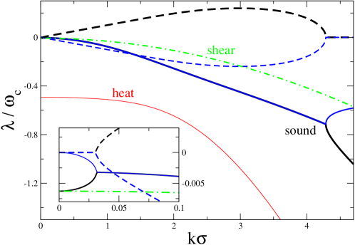
Figure 1: Eigenvalues spectrum $\lambda(k)$ of the dynamical matrix (9) calculated for $\phi=0.5$ and $\alpha=0.6$, namely in a strongly inelastic regime. The eigenvalues are normalized on the Enskog collision frequency $\omega_{c}$ so that on $y$ axis the ratio $\tau_{c}/\tau(k)=\lambda(k)/\omega_{c}$ between the microscopic time-scale of the model and the decay time of each mode can be directly read. Inset: zoom of the spectrum at small $k$.

We analyze the eigenvalues of ${\bf M}(k)$ in order to study the linear stability of the model and to characterize the range of validity of time-scales separation required by hydrodynamics. From the expression in Eq. (9) we learn that the shear modes are decoupled from all the others, and the typical time-scale of their decay simply reads as $\tau_{\perp}=(\gamma_{b}/m+\nu k^{2})^{-1}$. To obtain the typical time-scales for the fluctuations of the other hydrodynamic fields we solve, numerically, the equation $\textrm{Det}({\bf M}(k)-\lambda(k){\bf I})=0$, where ${\bf I}$ is the identity matrix. The eigenvalues spectrum thus found is shown in Fig. 1, for parameters of the model $\alpha=0.6$ and $\phi=0.5$. All parameters are calculated according to the formulas reported in A.

The study of hydrodynamic eigenvalues shows that, even in the case of a quite inelastic and dense regime, a range of scales where mesoscopic relaxation times are larger than the microscopic times exists and a hydrodynamic description can be attempted. In particular, comparing the eigenvalues $\lambda_{i}(k)$ with the Enskog frequency $\omega_{c}$ (which will be verified, below, to be a good estimate of the real frequency in simulations), see Fig. 1, we find, for each eigenvalue, the interval of values of $k$ where $\lambda_{i}/\omega_{c}<1$ is fulfilled. The subscript $i$ indicates eigenvalues related to heat ($i=H$), sound ($i=\pm$) and shear ($i=\perp$) modes. The range is narrower for the case of the mode dominated by temperature fluctuations (denominated “heat mode” in the Figure, red thin curve), while it is larger for shear modes (green dot-dashed lines) and modes dominated by longitudinal velocities and density fluctuations (here referred to as “sound modes”, black and blue thick curves, continuous for real part and dashed for imaginary part).

A general observation is that eigenvalues never have a positive real part, i.e. no instabilities are found, thanks to the presence of the external bath. Moreover, for the whole range of $k$ studied, the two “sound modes” - as usual - are complex conjugate, i.e. they propagate with a $k$-dependent velocity. A negative real part is always present, determining overall damping. At small values of $k$ one can identify a sound velocity $c$ by observing a linear relation $\textrm{Im}[\lambda_{\pm}]\sim ck$; instead the dispersion relation becomes strongly nonlinear at large $k$. Surprisingly, the study of sound eigenvalues shows that they have bifurcations at very small $k<k_{1}$ and very large $k>k_{2}$ wave-numbers, becoming in both limits pure real numbers, i.e. losing their propagating behavior. Those bifurcations are due to the external damping, ruled by $\gamma_{b}$: indeed in the limit $\gamma_{b}\to 0$ (keeping finite $\gamma_{b}T_{b}$), they disappear and the spectrum studied in [18, 20] is retrieved. Moreover, we find that the wavevector $k_{1}$ where the first bifurcation occurs, moves towards smaller values of $k$ when the dissipation is increased, namely when $\alpha$ is decreased (at fixed $\phi$) or when $\phi$ is increased (at fixed $\alpha$). Looking closely to the bifurcations, we see that one of the eigenvalues for “sound modes” approaches $0$ for $k\rightarrow 0$ (representing total number conservation) and the other tends to $-\gamma_{b}/m$ (as the shear one), see inset of Fig. 1. The bifurcation at large $k$ is perhaps non-physical, as it always falls out of the hydrodynamic range. For the eigenvalue of the heat mode we find that $\lambda_{H}(k=0)=-(3\gamma_{0}\omega_{c}+2\gamma_{b}/m)$. In the numerical setup used below, we have $k_{min}=2\pi/L>k_{1}$, so that the purely exponential decay of sound modes with large waves is never observed.

2.3 Stochastic description with fluctuating hydrodynamics

In order to fully account for the spatial fluctuations of the hydrodynamic fields and for the decay in time of such fluctuations we must add some noise terms to the linearized hydrodynamic equations: the basic assumption under fluctuating hydrodynamics is the same as for average (deterministic) hydrodynamics, i.e. a good separation of scales between hydrodynamic fields and microscopic degrees of freedom. In the linearized hydrodynamic equations the small scale fluctuations have been projected out, but their feedback on large scale fluctuations can be recovered by a proper addition of noise terms to dynamical equations:

$$\delta\dot{\bf a}({\bf k},t)={\bf M}(k)\delta{\bf a}({\bf k},t)+{\bf f}({\bf k},t).$$ (10)

A derivation from first principles of the noise ${\bf f}({\bf k},t)$ is beyond our scope. A kinetic theory with fluctuations has been recently proposed in [35, 36], for the homogeneous cooling regime, which is very different from our case. A similar treatment has been realized, only for the shear mode, in a driven case (random kicks without damping, i.e. $\gamma_{b}=0$) [37], showing that noise can be safely assumed to be white, at difference with the cooling regime. In such a case, with an additional but reasonable assumption on the two-particle velocity autocorrelation functions (namely, that such functions have only components in the hydrodynamic subspace), it is found that the fluctuation-dissipation relation for the internal part of the noise is satisfied, as already assumed in [25, 18]. Following those previous studies, we will consider valid such an assumption. Notice that it does not imply that fluctuation-dissipation relations will be satisfied by the whole noise, which is composed by internal as well as external contributions. In summary we write

$${\bf f}({\bf k},t)=\left(\begin{array}[]{c}0\\ \theta^{ex}({\bf k},t)+2ik/nd~{}\theta^{in}({\bf k},t)\\ \xi_{l}^{ex}({\bf k},t)+ik/\rho~{}\xi_{l}^{in}({\bf k},t)\\ \xi_{\perp}^{ex}({\bf k},t)+ik/\rho~{}\xi_{\perp}^{in}({\bf k},t)\}\end{array}\right),$$ (11)

where the two sources of noise for the hydrodynamic fields fluctuations are put in evidence: the first is the external contribution coming directly from the thermal bath, namely the stochastic force $\boldsymbol{\xi}_{b}$ of Eq. (2); the second is internal and enters through the constitutive equations for the heat flux and the pressure tensor. A detailed discussion on noises is presented in B. The external and internal noises are Gaussian with zero average. The variances of external noises can be obtained directly from Eqs. (2) and (4)

$$\langle\theta^{ex}({\bf k},t)\theta^{ex}({\bf k}^{\prime},t^{\prime})\rangle = \frac{4mT_{g}}{dn}\frac{2\gamma_{b}T_{b}}{m}\delta(t-t^{\prime})\delta({\bf k}+{\bf k}^{\prime})$$

$$\langle\xi^{ex}_{l}({\bf k},t)\xi^{ex}_{l}({\bf k}^{\prime},t^{\prime})\rangle = \langle\xi^{ex}_{\perp}({\bf k},t)\xi^{ex}_{\perp}({\bf k}^{\prime},t^{\prime})\rangle=\frac{1}{n}\frac{2\gamma_{b}T_{b}}{m}\delta(t-t^{\prime})\delta({\bf k}+{\bf k}^{\prime}),$$ (12)

while the variances of the internal contributions are obtained by imposing the fluctuation-dissipation theorem (see B for details):

$$\langle\theta^{in}({\bf k},t)\theta^{in}({\bf k}^{\prime},t^{\prime})\rangle = 2\kappa T_{g}^{2}\delta(t-t^{\prime})\delta({\bf k}+{\bf k}^{\prime})$$

$$\langle\xi^{in}_{l}({\bf k},t)\xi^{in}_{l}({\bf k}^{\prime},t^{\prime})\rangle = 2nm\nu_{l}T_{g}\delta(t-t^{\prime})\delta({\bf k}+{\bf k}^{\prime})$$

$$\langle\xi^{in}_{\perp}({\bf k},t)\xi^{in}_{\perp}({\bf k}^{\prime},t^{\prime})\rangle = 2nm\nu T_{g}\delta(t-t^{\prime})\delta({\bf k}+{\bf k}^{\prime}).$$ (13)

The internal and external noises are uncorrelated

$$\langle\theta^{ex}({\bf k},t)\theta^{in}({\bf k}^{\prime},t^{\prime})\rangle=\langle\xi_{l}^{ex}({\bf k},t)\xi_{l}^{in}({\bf k}^{\prime},t^{\prime})\rangle=\langle\xi_{\perp}^{ex}({\bf k},t)\xi_{\perp}^{in}({\bf k}^{\prime},t^{\prime})\rangle=0.$$ (14)

The hydrodynamic analysis of model (2) consists, then, in solving the system of coupled linear Langevin equations (10). In particular we are interested in finding the explicit forms of the static and dynamical structure factors, respectively

$$S_{ab}({\bf k})=\lim_{t\to\infty}\frac{1}{V}\langle\delta a({\bf k},t)\delta b({-\bf k},t)\rangle,$$ (15)

and

$$S_{ab}({\bf k},\omega)=\int_{-\infty}^{\infty}S_{ab}({\bf k},t)e^{-i\omega t},$$ (16)

where

$$S_{ab}({\bf k},t)=\lim_{t^{\prime}\to\infty}\frac{1}{V}\langle\delta a({\bf k},t^{\prime}+t)\delta b({-\bf k},t^{\prime})\rangle.$$ (17)

3 Out-of-equilibrium correlations: Static and Dynamical structure factors

It is well known that spatially extended correlations develop in the non-equilibrium stationary state of a driven granular fluid [18, 20]. In particular, the velocity correlator $\langle{\bf u}({\bf k})\cdot{\bf u}(-{\bf k})\rangle$, where the average $\langle\ldots\rangle$ is taken over noises, can be written as

$$\langle{\bf u}({\bf k})\cdot{\bf u}(-{\bf k})\rangle=\langle u_{\parallel}({\bf k})u_{\parallel}(-{\bf k})\rangle+\langle u_{\perp}({\bf k})u_{\perp}(-{\bf k})\rangle,$$ (18)

with the cross terms $\langle u_{\perp}({\bf k})u_{\parallel}(-{\bf k})\rangle=0$. The two terms on the right of Eq. (18) can be studied separately.

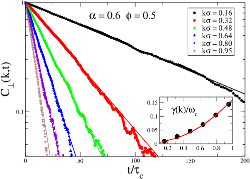
Figure 2: $C_{\perp}(k,t)$ for $\alpha=0.6$ and $\phi=0.5$ and several values of $k\sigma$ measured in numerical simulations, together with exponential fits (continuous curves). In the inset the quantity $\gamma(k)$ obtained from the fits is reported, rescaled with the collision frequency $\omega_{c}$, together with the parabolic fit via the formula $\gamma(k)=\gamma_{b}+\nu k^{2}$ (continuous red line).

3.1 Shear modes

According to the matrix (9) the shear modes are decoupled from the others in the linear approximation and their dynamics obeys a simple Langevin equation

$$\dot{u}_{\perp}({\bf k},t)=-(\gamma_{b}+\nu k^{2})u_{\perp}({\bf k},t)+\xi_{\perp}^{ex}({\bf k},t)+ik/n~{}\xi_{\perp}^{in}({\bf k},t),$$ (19)

where, from now on, we put $m=1$ in all formulas. The effect of internal and external noises is equal to a single complex noise $\xi_{\perp}({\bf k},t)=\xi_{\perp}^{ex}({\bf k},t)+ik/n~{}\xi_{\perp}^{in}({\bf k},t)$ with variance:

$$V^{-1}\langle\xi_{\perp}({\bf k},t)\xi_{\perp}(-{\bf k},t^{\prime})\rangle~{}=~{}\frac{2}{n}\left(T_{b}\gamma_{b}+\nu T_{g}k^{2}\right)\delta(t-t^{\prime}).$$ (20)

From this, the equal-time correlator $\langle u_{\perp}({\bf k})u_{\perp}(-{\bf k})\rangle$ can be easily calculated:

$$nS_{\perp}(k)=N^{-1}\langle|u_{\perp}(k)|^{2}\rangle=\frac{\gamma_{b}T_{b}+\nu k^{2}T_{g}}{\gamma_{b}+\nu k^{2}}=T_{g}+\frac{(T_{b}-T_{g})}{1+\xi^{2}k^{2}},$$ (21)

with $\xi^{2}=\nu/\gamma_{b}$. The meaning of the above equation is clear: the small length-scale physics, which depends on the inelastic collisions, is related to the granular temperature $T_{g}$, while at large distances there are correlations with finite amplitude $T_{b}-T_{g}$ and extent $\xi$. Notice that in the limit $\gamma_{b}\to 0$, keeping $\gamma_{b}T_{b}$ finite, from Eq. (21) one obtains the result of Ref. [18], where $S_{\perp}(k)\sim 1/k^{2}$ and long range correlations are observed. A similar power law behaviour is also observed in molecular fluids under shear [7]. The different result we obtain in our model is due to the intrinsic cut-off introduced by the viscous drag $\gamma_{b}>0$. Indeed, the finite extent of correlations is even more clear when Eq. (21) is written in real space, yielding the spatial correlation function $G_{\perp}({\bf r})$, which reads:

$$nG_{\perp}({\bf r})=T_{g}\delta^{(2)}({\bf r})+(T_{b}-T_{g})\frac{K_{0}(r/\xi)}{\xi^{2}},$$ (22)

where $K_{0}(x)$ is the 2nd kind modified Bessel function that, for large distances, decays exponentially

$$K_{0}(r/\xi)\approx\sqrt{\frac{\pi}{2}}\frac{e^{-r/\xi}}{(r/\xi)^{1/2}}.$$ (23)

At equilibrium, namely when collisions are elastic and $T_{g}=T_{b}$, equipartition between modes is perfectly fulfilled and the structure factor becomes flat, i.e. $S_{\perp}(k)=T_{b}$. Differently, in the granular case, where $T_{g}\neq T_{b}$, equipartition breaks down and from Eq. (21) we have that $S_{\perp}\to T_{b}$ for small $k$ and $S_{\perp}\to T_{g}$ for large $k$. We see here that out of equilibrium the quantity $\xi=\sqrt{\nu/\gamma_{b}}$ measures the range of static correlations of the vorticity field. The behaviour described above is in good agreement with experimental results obtained for driven granular fluids, as reported in [38] and, more recently, in [32].

From Eq. (19) we also find that fluctuations decay exponentially

$$\langle u_{\perp}(k,t)u_{\perp}(-k,0)\rangle\sim S_{\perp}(k)~{}e^{-(\gamma_{b}+\nu k^{2})t},$$ (24)

with a characteristic time $\tau(k)=\gamma(k)^{-1}=(\gamma_{b}+\nu k^{2})^{-1}$. Such a behavior is also observed for elastic fluids, with the only difference that in that case $S_{\perp}(k)=T_{b}/n$ is constant. The length-scale $\xi=\sqrt{\nu/\gamma_{b}}$ can be therefore always connected to dynamical properties of the system. What is peculiar of the out-of-equilibrium regime is that the so defined $\xi$ also represents the extent of correlations of the vorticity field, thus establishing a remarkable link between static correlations and dynamical ones.

In Fig. 2 are reported the correlators $C_{\perp}(k,t)=\langle u_{\perp}(k,t)u_{\perp}(-k,0)\rangle/\langle|u_{\perp}(k)|^{2}\rangle$ for different values of $k$ and the same packing fraction measured in numerical simulations. Let us notice that the decay of $\langle u_{\perp}(k,t)u_{\perp}(-k,0)\rangle$ is always exponential: we can therefore a-posteriori support the validity of linear hydrodynamics, from which the Langevin equations for shear modes is obtained. By interpolating with a parabola the characteristic time $\tau(k)$ as a function of $k$, see inset of Fig. (2), we obtain the shear viscosity $\nu$. Let us stress the deep connection between statics and dynamics in the out-of-equilibrium regime: inserting the values of $\nu$ obtained from the dynamics into Eq. (21), we find curves that well superimpose the numerical data for $\langle u_{\perp}(k)u_{\perp}(-k)\rangle$, (see Fig. 3). The values of $\nu$ obtained from the dynamics of shear modes can be independently obtained as fit parameters of $S_{\perp}(k)$ via Eq. (21). The values of $\nu$ obtained with the two different procedures are compatible, as can be seen from Tab. 1. They are also reasonably close to the dense EHS predictions, presented in the same Table.

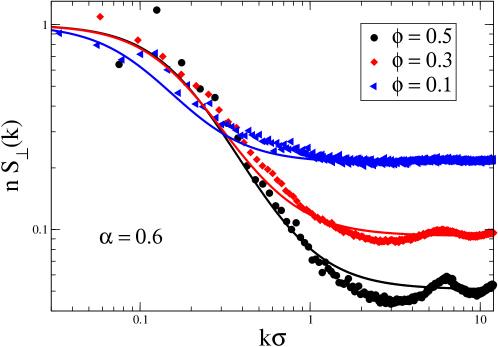
Figure 3: Shear modes structure factor $nS_{\perp}(k)$ at different packing fractions for $\alpha=0.6$. Full curves are drawn by inserting into Eq. (21) the values of $\nu$ obtained from the decay of dynamical correlators.

$\phi$	Statics	Dynamics	dense EHS
0.1	0.0062	0.0072	0.0111
0.2	0.0036	0.0041	0.0052
0.3	0.0025	0.0031	0.0039
0.4	0.0026	0.0027	0.0037
0.5	0.0020	0.0028	0.0041

Table 1: Comparison of the shear viscosity obtained from statics (fit via Eq. (21)), dynamics (fit via Eq. (24)) and dense EHS approximation.

3.2 Longitudinal modes

3.2.1 Static correlations

The same considerations discussed above for shear modes also hold for the other hydrodynamic modes, which are coupled each other. In order to study their behaviour we have to take into account all the elements of the dynamical matrix. In particular, the matrix of static structure factors ${\bf S}({\bf k})$ with elements $S_{ab}(k)$, is obtained solving the following linear system:

$${\bf M}(k){\bf S}(k)+{\bf S}^{\dagger}(k){\bf M}^{\dagger}(k)+{\bf C}(k)=0,$$ (25)

where the matrix of noises ${\bf C}(k)$ is such that:

$$V^{-1}\langle{\bf f}({\bf k},t)\otimes{\bf f}(-{\bf k},t^{\prime})\rangle={\bf C}({\bf k})\delta(t-t^{\prime}).$$ (26)

Here

$${\bf C}({\bf k})=\textrm{diag}\left[0,\frac{2T_{g}}{dn}\left(4T_{b}\gamma_{b}+2D_{T}T_{g}k^{2}\right),\frac{2}{n}\left(T_{b}\gamma_{b}+\nu_{l}T_{g}k^{2}\right),\frac{2}{n}\left(T_{b}\gamma_{b}+\nu T_{g}k^{2}\right)\right],$$ (27)

where $\textrm{diag}[x,y,z,w]$ denotes a diagonal matrix with elements $x,y,z,w$.

The expression of the longitudinal structure factor,

$$nS_{\parallel}(k)=N^{-1}\langle|u_{l}(k)|^{2}\rangle,$$ (28)

turns out to be the ratio between two even polynomial functions of the $6-$th order in $k$:

$$nS_{\parallel}(k)=\frac{S_{0}+S_{2}k^{2}+S_{4}k^{4}+S_{6}k^{6}}{S_{0}^{\prime}+S_{2}^{\prime}k^{2}+S_{4}^{\prime}k^{4}+S_{6}^{\prime}k^{6}}.$$ (29)

In the above expression eight constants have been introduced, which depend in a complicate manner by all the parameters of the system. Let us focus here on the asymptotic behavior of $S_{\parallel}(k)$ at large and small values of $k$. From Eq. (3) there follows the relation $d\gamma_{0}\omega_{c}/2=\gamma_{b}(T_{b}-T_{g})/T_{g}$, which allows us to recast the series expansion around $k=0$ of the expression in Eq. (29) in the form

$$nS_{\parallel}(k\rightarrow 0)\simeq T_{b}-(T_{b}-T_{g})\xi_{l}^{2}k^{2}+\mathcal{O}(k^{2}),$$ (30)

with

$$\xi_{l}^{2}=\frac{\nu^{*}_{l}}{\gamma_{b}}=\frac{1}{\gamma_{b}}\left[\nu_{l}+\frac{\gamma_{b}T_{b}}{nT_{g}(\gamma_{b}+\gamma_{0}\omega_{c})(2\gamma_{b}+3\gamma_{0}\omega_{c})}\left(\frac{4p^{2}}{d^{2}nT_{g}}+\frac{2g(n)p}{3d}\right)\right].$$ (31)

Up to $\mathcal{O}(k^{2})$ the expression in Eq. (30) is equivalent to

$$nS_{\parallel}(k)=T_{g}+\frac{(T_{b}-T_{g})}{1+\xi_{l}^{2}~{}k^{2}},$$ (32)

namely a form analogous to the structure factor we found for the shear modes. In Fig. 4 we show the static structure factors for different packing fractions. Again, notice that in the limit $\gamma_{b}\to 0$ with $\gamma_{b}T_{b}$ finite, the behaviour $S_{\parallel}(k)\sim 1/k^{2}$ found in [18] is recovered. Albeit the above expression is in principle only valid for low $k$ values, it captures also the large $k$ limit, when fine oscillations are disregarded. Indeed, expanding Eq. (29) for large $k$ values we find:

$$nS_{\parallel}(k\rightarrow\infty)\simeq T_{g}+\frac{(T_{b}-T_{g})}{\xi_{l}^{2}k^{2}}.$$ (33)

Such a discussion shows that even for longitudinal modes the viscosity $\nu_{l}$ is related to a finite correlation length, measurable from static velocity correlations when the system is out of equilibrium with $T_{g}<T_{b}$. The behavior of that length when the packing fraction is increased will be discussed in the last section.

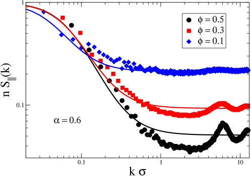
Figure 4: Longitudinal modes structure factor $nS_{\parallel}(k)$ at different packing fractions, for $\alpha=0.6$. Full curves are drawn inserting into Eq. (32) the values of $\xi_{l}$, defined in Eq. (31), obtained from best fits of the dynamical structure factors.

3.2.2 Dynamical correlations

Dynamical correlations for longitudinal modes are less simple than those for the shear mode, since they are given by a superposition of different (real and imaginary) exponentials. The dynamical structure factors are obtained by solving the equation of motion (10), which, in the frequency domain, reads as

$$\widetilde{{\bf M}}({\bf k},\omega)\delta\tilde{{\bf a}}({\bf k},\omega)=\tilde{{\bf f}}({\bf k},\omega),$$ (34)

where

$$\widetilde{{\bf M}}({\bf k},\omega)=i\omega{\bf I}-{\bf M}({\bf k}),$$ (35)

with ${\bf I}$ the identity matrix,

$$\delta\tilde{a}({\bf k},\omega)=\int_{-\infty}^{\infty}dt~{}\delta a({\bf k},t)e^{-i\omega t},$$ (36)

and

$$V^{-1}\langle\tilde{{\bf f}}({\bf k},\omega)\otimes\tilde{{\bf f}}(-{\bf k},\omega^{\prime})\rangle={\bf C}({\bf k})\delta(\omega+\omega^{\prime}),$$ (37)

${\bf C}(k)$ being defined in Eq. (27). Multiplying Eq. (34) on the left by $\widetilde{{\bf M}}^{-1}(k,\omega)$ and on the right by $\delta\tilde{{\bf a}}^{T}(-k,-\omega)$ (where $X^{T}$ denotes the transpose of $X$) and averaging over the noise, we obtain the matrix of dynamical structure factors

$${\bf S}(k,\omega)=V^{-1}\langle\widetilde{{\bf M}}^{-1}(k,\omega)\tilde{{\bf f}}(k)\delta\tilde{{\bf a}}^{T}(-k,-\omega)\rangle=\widetilde{{\bf M}}^{-1}(k,\omega){\bf C}(k)[\widetilde{{\bf M}}^{T}(-k,-\omega)]^{-1},$$ (38)

where in the last equality we have used the Hermitian conjugate of Eq. (34) and the relation (37).

The dynamical structure factors $S_{nn}(k,\omega)$ and $S_{\parallel}(k,\omega)$ take the explicit forms

$$S_{nn}(k,\omega)=n^{2}k^{2}\left(\frac{\left[\omega^{2}+(2\gamma_{b}+D_{T}k^{2}+3\gamma_{0}\omega_{c})^{2}\right](\frac{2\gamma_{b}T_{b}}{n}+\frac{2\nu k^{2}T_{g}}{n})+k^{2}\left(\frac{p}{nT_{g}}\right)^{2}\left(\frac{4D_{T}T_{g}^{2}k^{2}}{nd}+\frac{8T_{g}\gamma_{b}T_{b}}{nd}\right)}{|\det\widetilde{{\bf M}}|^{2}}\right),$$

where

$$|\det\widetilde{{\bf M}}|^{2}=\left[-\omega^{2}(3\gamma_{0}\omega_{c}+D_{T}k^{2}+\nu k^{2}+3\gamma_{b})+k^{2}\left((2\gamma_{b}+3\gamma_{0}\omega_{c})v_{T}^{2}-\frac{g(n)p\gamma_{0}\omega_{c}}{n}+v_{T}^{2}D_{T}k^{2}\right)\right]^{2}$$

$$+\left\{\omega^{3}-\omega\left[\gamma_{b}(2\gamma_{b}+3\gamma_{0}\omega_{c})+k^{2}\left(D_{T}(\nu k^{2}+\gamma_{b})+\nu(2\gamma_{b}+3\gamma_{0}\omega_{c})+\frac{2p^{2}}{dn^{2}mT_{g}}+v_{T}^{2}\right)\right]\right\}^{2},$$

and

$$S_{\parallel}(k,\omega)=\frac{\omega^{2}}{n^{2}k^{2}}S_{nn}(k,\omega).$$ (41)

$\phi=0.5$
	$\alpha=0.6$		$\alpha=0.8$
	Sim	dense EHS	Sim	dense EHS
$T_{g}$	0.051	0.0416	0.066	0.0603
$\omega_{c}$	179	160	181	181
$\phi=0.3$
	$\alpha=0.6$		$\alpha=0.8$
	Sim	dense EHS	Sim	dense EHS
$T_{g}$	0.093	0.0829	0.125	0.1185
$\omega_{c}$	79	83	85	85
$\phi=0.1$
	$\alpha=0.6$		$\alpha=0.8$
	Sim	dense EHS	Sim	dense EHS
$T_{g}$	0.212	0.2055	0.286	0.2820
$\omega_{c}$	26	25	29	28

Table 2: Comparison of theoretical predictions of Eqs. (3) and (43) and numerical results for $T_{g}$ and $\omega_{c}$.

All the coefficients appearing in these expressions can be evaluated within the dense EHS approximation, so that Eq. (41) can be used in order to obtain $\nu_{l}$ and $D_{T}$ from the numerical data. Clearly the writing of physical quantities, such as $v_{T}^{2}=(\partial p/\partial n)_{T}$ or $p$ itself, with dense EHS formulas leads to systematic errors. The amplitude of this error can be estimated for instance by comparing the theoretical prediction of dense EHS collision frequency with the collision frequency measured in simulations. In Table 2 are listed both dense EHS and numerical collision frequencies at different packing fractions. Again it is found that the dense EHS prediction is quite good.

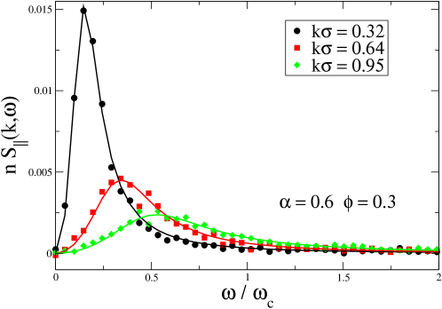
Figure 5: Dynamical structure factor $nS_{\parallel}(k,\omega)$ at fixed packing fractions $\phi$ and different momenta. Identifying a characteristic time $\tau_{peak}$ with the frequency of the maximum of the curve we see that $\tau_{c}/\tau_{peak}=\omega/\omega_{c}$ grows with the wave-vector, namely longitudinal modes of higher momentum decay faster. Continuous lines show the best fit results via Eq. (41), with $D_{T}$ and $\nu_{l}$ as fitting parameters and all other coefficients fixed with the dense EHS predictions.

In order to obtain the longitudinal viscosity and the thermal diffusion coefficient, we fit our numerical data for the longitudinal modes using Eq. (41), where all parameters but $\nu_{l}$ and $D_{T}$ are fixed to the dense EHS values and $T_{g}$ is the one measured in simulations. In Fig. 5 $S_{\parallel}(k,\omega)$ is shown for different values of $k$ and fixed $\phi=0.5$, together with the best fit curves. The values of $\nu_{l}$ and $D_{T}$ so obtained, together with those computed within the dense EHS approximation, for different values of $\phi$ and $\alpha$, are reported in Table 3 and within errors are found independent of $k$. This fact represents an a-posteriori check that we are in the regime of validity of linearized hydrodynamics. Indeed, in Eqs. (41) and (3.2.2) $\nu_{l}$ appears as $k$-independent variable. Only at low packing fraction we observe a dependence on $k$. This is perhaps due to diluteness, which implies too large mean free path or mean free time with respect to mesoscopic scales.

In Fig. 6 we also show the time decay of the dynamical structure factor. It can be appreciated, in the time domain, the superposition of different real and imaginary exponentials, which determines a mix of damping and propagation.

The dynamical structure factor at fixed $k$ and different packing fractions is reported in Fig. 7: it is remarkable the observation of a time-scale, individuated by the peak frequency of $S_{\parallel}(k,\omega)$, which increases as the packing fraction is increased. Such behaviour is consistent with the observation, discussed in details below, of a growth of the correlation lengths defined above, together with the packing fraction.

$\phi=0.5$
	$\alpha=0.6$		$\alpha=0.8$
	$D_{T}$	$\nu_{l}$	$D_{T}$	$\nu_{l}$
Fit Results: $k\sigma=0.5$	0.019	0.0053	0.020	0.011
$k\sigma=0.6$	0.020	0.0046	0.018	0.011
$k\sigma=0.8$	0.021	0.0055	0.019	0.0076
dense EHS	0.018	0.0081	0.021	0.0090
$\phi=0.3$
	$\alpha=0.6$		$\alpha=0.8$
	$D_{T}$	$\nu_{\rm l}$	$D_{T}$	$\nu_{\rm l}$
Fit Results: $k\sigma=0.4$	0.017	0.0052	0.013	0.0098
$k\sigma=0.5$	0.020	0.0058	0.013	0.0091
$k\sigma=0.6$	0.017	0.0058	0.015	0.0079
dense EHS	0.018	0.0057	0.021	0.0066
$\phi=0.1$
	$\alpha=0.6$		$\alpha=0.8$
	$D_{T}$	$\nu_{\rm l}$	$D_{T}$	$\nu_{\rm l}$
Fit Results: $k\sigma=0.2$	0.039	0.016	0.021	0.023
$k\sigma=0.3$	0.028	0.016	0.019	0.018
$k\sigma=0.4$	0.018	0.013	0.0096	0.016
dense EHS	0.048	0.012	0.056	0.014

Table 3: Comparison of theoretical predictions of Eqs. (46-50) and fit results via Eqs. (41) for $D_{T}$ and $\nu_{l}$.

We conclude this section by stressing the remarkable agreement between numerical $S_{\parallel}(k)$ data and the expression of Eq. (32), see Fig. 4, with $\nu_{l}$ measured from dynamics and the renormalization term entering the definition of $\nu_{l}^{*}$ (see Eq. (31)) calculated within the dense EHS approximation and reported in Table 3.

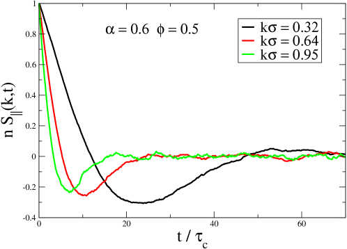
Figure 6: Dynamical structure factor $nS_{\parallel}(k,t)$ at fixed packing fraction $\phi$ and different momenta. The observed oscillations are in agreement with the eigenvalues spectrum in the interval of momenta considered: the eigenvalues of sound modes are complex conjugate, thus producing an oscillatory relaxation.

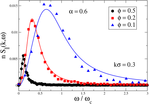
Figure 7: Dynamical structure factor $nS_{\parallel}(k,\omega)$ at fixed momentum $k$ and different packing fractions. Identifying a characteristic time $\tau_{peak}$ with the frequency of the maximum of the curve we see that $\tau_{c}/\tau_{peak}=\omega/\omega_{c}$ grows when the packing fraction is lowered, namely sound modes decays faster compared to the microscopic time-scale. Continuous lines show the best fit results via Eq. (41), with $D_{T}$ and $\nu_{l}$ as fitting parameters and all other coefficients fixed with the dense EHS predictions.

4 Summary and conclusions: transport coefficients and non-equilibrium correlation lengths

In conclusion, we have studied both static and dynamical correlations for hydrodynamic fluctuations of the velocity and density fields: indeed we recall Eq. (41) which gives a direct relation between density and longitudinal velocity structure factors. A main comment concerns the good success of analytical predictions: comparison with simulations shows a fair agreement up to $\phi=0.5$, with values for most of the parameters directly given in the dense EHS approximation. This signals a success of the three main ingredients: 1) dense EHS theory for transport coefficients, working even at quite high densities, 2) scale separation and granular hydrodynamics, and 3) prescription of Eqs. (12-14) for the hydrodynamic noise. The last ingredient is perhaps the most interesting, if one considers how hard is the characterization in simple terms of non-equilibrium systems. Moreover, the assumption of white internal noise is less obvious than in the case of simple random kicks without drag [37]: in that case, the absence of drag ($\gamma_{b}=0$) implies a relaxation time at large scales, $k\to 0$, which diverges, making a solid base for assuming fast the relaxation of noise due to microscopic degrees of freedom. In our model, in principle, the drag could be large enough to make even large scales fast, making difficult to define hydrodynamic fields. Recent experiments show that, even if that could be a realistic situation, this does not change dramatically the qualitative behavior of structure factors [32].

One of the main results of our study is the presence of spatial order in the form of non-equilibrium velocity correlations. This should be related to the slowing-down of the dynamics with increasing packing fraction in granular systems [39, 20], and with the existence of a time-scale growing with the density, as observed in [11]. As discussed in Sec. 3, in our model the competition between different relaxation mechanisms given by the kinematic and longitudinal viscosities $\nu$ and $\nu_{l}$ and the thermostat damping $\gamma_{b}$ give place to a couple of length-scales characterizing non-equilibrium structure factors: $\xi=\sqrt{\nu/\gamma_{b}}$ and $\xi_{l}=\sqrt{\nu_{l}^{*}/\gamma_{b}}$. The first trivial observation is that allowing $\gamma_{b}\rightarrow 0$ such lengths diverge. It means that, according to the prediction of [18], the largest-scale correlations are always equal to the size of the system, which is the largest size available. In our model there is a cut-off on such correlations imposed by the viscous drag $\gamma_{b}>0$ due to the interaction with the thermal bath. The existence of such a cut-off, which represents a fixed parameter at different packing fractions, allows us to show that by increasing the packing fraction the extent of correlations is effectively increased. While the absolute value of $\xi$ is only slightly enhanced when $\phi$ is increased, as also observed in experiments in [38], we stress that, in order to appreciate the physical meaning of such length at different densities, one has to compare it with the microscopic relevant spatial scale in the system, which is given by the mean free path of the particles $\lambda_{0}=\sqrt{\pi}\sigma/(8\phi\chi(\phi))$ and which also changes with the packing fraction. Then one finds that $\xi/\lambda_{0}$ is remarkably increased at high densities, as can be seen in Fig. 8, and also in recent experiments [32]. We may summarize the observed phenomenon saying that the higher is the packing fraction the higher must be the number of intermediate scattering events between two different particles in order to decorrelate their velocities. This scenario could be reflected in transitions of dynamical origin, at higher packing fractions [40, 41, 42, 39].

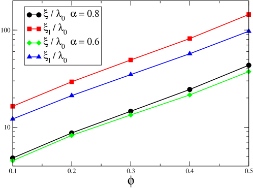
Figure 8: Correlation lengths $\xi$ and $\xi_{l}$ rescaled with the mean free path $\lambda_{0}$, for different packing fractions and several values of the restitution coefficient. The extent of correlations grows exponentially with the packing fraction. Notice also that, at fixed $\phi$, $\xi$ and $\xi_{l}$ are larger for higher values of $\alpha$. However the amplitude of correlations, ruled by $T_{b}-T_{g}$, is smaller, see Eqs. (21) and (30).

Appendix A Dense EHS formulas for hydrodynamic coefficients

The definitions of the parameters entering the matrix ${\bf M}$ are

$$v_{T}^{2} = \left[\frac{\partial p}{\partial\rho}\right]_{T},$$ (42)

$$\omega_{c} = \Omega_{d}\chi(\phi)n\sigma^{d-1}\sqrt{\frac{T_{g}}{\pi m}}$$ (43)

$$g(\phi) = 2\left(1+\frac{\phi}{\chi(\phi)}\frac{\partial\chi(\phi)}{\partial\phi}\right).$$ (44)

In the dense EHS approximation the pressure $p$ can be written as

$$p(n)=nT_{g}\left(1+\frac{\Omega_{d}\chi n\sigma^{d}}{2d}\frac{1+\alpha}{2}\right),\\$$

which in $d=2$ reads as

$$p(\phi)=\frac{4}{\pi\sigma^{2}}\phi~{}T_{g}(1+\phi\chi(\phi)(1+\alpha)),$$ (45)

where has been made use of the relation between packing fraction and density $n=4\phi/(\pi\sigma^{2})$, and of the definition $\Omega_{d}=2\pi^{d/2}/\Gamma(d/2)$ with $d=2$. Notice also that we have taken into account the correction due to the inelasticity, as given in [43]. There are dense EHS formulas also for the dependence of the diffusion coefficients on the packing fraction and the granular temperature. In the following such formulas are written for a 2d system. In this case, we use the Verlet-Levesque approximation for the pair correlation function at contact: $\chi(\phi)=(1-7\phi/16)/(1-\phi)^{2}$.

Shear viscosity:

$$\eta_{E}=\nu_{0}\left[\frac{1}{\chi(\phi)}+2\phi+\left(1+\frac{8}{\pi}\right)\chi(\phi)\phi^{2}\right],$$ (46)

with

$$\nu_{0}=\frac{1}{2\sigma}\left(\frac{mT_{g}}{\pi}\right)^{1/2}.$$ (47)

Bulk viscosity:

$$\zeta_{E}=\frac{8\phi^{2}\chi(\phi)}{\pi\sigma}\left(\frac{mT_{g}}{\pi}\right)^{1/2}.$$ (48)

Thermal diffusivity:

$$\kappa_{E}=\kappa_{0}\left[\frac{1}{\chi(\phi)}+3\phi+\left(\frac{9}{4}+\frac{4}{\pi}\right)\chi(\phi)\phi^{2}\right],$$ (49)

with

$$\kappa_{0}=\frac{2}{\sigma}\left(\frac{T_{g}}{\pi m}\right)^{1/2}.$$ (50)

Appendix B Noises

In this appendix we present a detailed discussion of the noise terms appearing in the fluctuating hydrodynamic equations (10). Let us start from the external noises, which can be simply obtained from Eqs. (2) and (4). We find that the noise contributions to the equations for the velocity and temperature fields are, respectively

$$\boldsymbol{\xi}^{ex}({\bf r},t) = \frac{1}{n}\sum_{i}\boldsymbol{\xi}_{b,i}(t)\delta({\bf r}-{\bf r}_{i}(t))$$ (51)

$$\theta^{ex}({\bf r},t) = \frac{2m}{dn}\sum_{i}{\bf v}_{i}(t)\cdot\boldsymbol{\xi}_{b,i}(t)\delta({\bf r}-{\bf r}_{i}(t)).$$ (52)

These are Gaussian noises with variances

$$\langle\xi^{ex}_{\alpha}({\bf r},t)\xi^{ex}_{\beta}({\bf r^{\prime}},t^{\prime})\rangle = \frac{1}{n}\frac{2\gamma_{b}T_{b}}{m}\delta_{\alpha\beta}\delta(t-t^{\prime})\delta({\bf r}-{\bf r^{\prime}})$$

$$\langle\theta^{ex}({\bf r},t)\theta^{ex}({\bf r^{\prime}},t^{\prime})\rangle = \frac{4mT_{g}}{dn}\frac{2\gamma_{b}T_{b}}{m}\delta(t-t^{\prime})\delta({\bf r}-{\bf r^{\prime}}).$$ (53)

In order to describe the local spontaneous microscopic fluctuations of the fluid, we also include in our description internal conserved Gaussian noises $\boldsymbol{\theta}^{in}$ and $\boldsymbol{\xi}^{in}$, which enter the constitutive equations for ${\bf J}$ and $\boldsymbol{\Pi}$, respectively

$${\bf J} = -\kappa\boldsymbol{\nabla}T+\boldsymbol{\theta}^{in}$$ (54)

$$\boldsymbol{\Pi} = p{\bf 1}-\eta\left[\boldsymbol{\nabla}{\bf u}+\left(\boldsymbol{\nabla}{\bf u}\right)^{{\dagger}}\right]+\left(\frac{2}{d}\eta-\zeta\right){\bf 1}\boldsymbol{\nabla}\cdot{\bf u}+\boldsymbol{\xi}^{in},$$ (55)

where $\kappa$ is the heat conductivity, $p$ is the local pressure, ${\bf 1}$ the unit tensor, $\eta$ the shear viscosity and $\zeta$ the bulk viscosity. The amplitudes of such noises are obtained from the fluctuation-dissipation theorem [4, 5, 44]

$$\langle\xi^{in}_{\alpha\beta}({\bf r},t)\xi^{in}_{\gamma\delta}({\bf r^{\prime}},t^{\prime})\rangle = 2T_{g}[\eta(\delta_{\alpha\gamma}\delta_{\beta\delta}+\delta_{\alpha\delta}\delta_{\beta\gamma})+\left(\zeta-\frac{2}{d}\eta\right)\delta_{\alpha\beta}\delta_{\gamma\delta}]\delta(t-t^{\prime})\delta({\bf r}-{\bf r^{\prime}})$$

$$\langle\theta^{in}_{\alpha}({\bf r},t)\theta^{in}_{\beta}({\bf r^{\prime}},t^{\prime})\rangle = 2\kappa T_{g}^{2}\delta_{\alpha\beta}\delta(t-t^{\prime})\delta({\bf r}-{\bf r^{\prime}}).$$ (56)

Notice that, for granular systems, Eq. (54) should be modified, adding the term $-\mu\nabla n$ on the rhs, which takes into account the contribution to the heat current due to density gradients [45]. However, the transport coefficient $\mu$ is very small for driven systems [46], and therefore we have neglected this contribution.

Linearization

In order to obtain the linear approximation of the hydrodynamic equations, we consider how a homogeneous fluctuation of the temperature relaxes around its stationary value $T_{g}$. Therefore we start by linearizing Eq. (5) around $T_{g}$, with $n({\bf r},t)=n,{\bf u}=0,T({\bf r},t)=T(t)$, and obtain

$$\delta\dot{T}(t)=-(2\gamma_{b}/m+3\gamma_{0}\omega_{c})\delta T(t).$$ (57)

Notice that the quantity $-(2\gamma_{b}/m+3\gamma_{0}\omega_{c})$ coincides with the heat mode eigenvalue $\lambda_{H}(k=0)$.

Next, taking the linear terms around the non-equilibrium steady state in Eqs. (5), introducing the external noises (51) and (52), and using Eqs. (54) and (55), we obtain

$$\partial_{t}\delta n({\bf r},t) = -n\boldsymbol{\nabla}\cdot{\bf u}({\bf r},t)$$

$$\partial_{t}{\bf u}({\bf r},t) = -\frac{1}{\rho}\boldsymbol{\nabla}p({\bf r},t)+\nu\nabla^{2}{\bf u}({\bf r},t)+(\nu_{l}-\nu)\boldsymbol{\nabla}\boldsymbol{\nabla}\cdot{\bf u}({\bf r},t)$$ (58)

$$- \frac{\gamma_{b}}{m}{\bf u}({\bf r},t)-\frac{1}{\rho}\boldsymbol{\nabla}\cdot\boldsymbol{\xi}^{in}({\bf r},t)+\boldsymbol{\xi}^{ex}({\bf r},t)$$

$$\partial_{t}\delta T({\bf r},t) = \frac{2\kappa}{nd}\nabla^{2}\delta T({\bf r},t)-\frac{2p}{nd}\boldsymbol{\nabla}\cdot{\bf u}({\bf r},t)-\frac{\gamma_{0}\omega_{c}g(n)T_{g}}{n}\delta n$$

$$- 2\frac{\gamma_{b}}{m}\delta T({\bf r},t)-3\gamma_{0}\omega_{c}~{}\delta T({\bf r},t)-\frac{2}{nd}\boldsymbol{\nabla}\cdot\boldsymbol{\theta}^{in}({\bf r},t)+{\theta}^{ex}({\bf r},t),$$

with $\rho\nu=\eta$ and $\rho\nu_{l}=2\eta(d-1)/d+\zeta$.

The velocity field ${\bf u}$ can be split in longitudinal and transverse components ${\bf u}={\bf u}_{l}+{\bf u}_{\perp}$, where ${\bf\nabla}\cdot{\bf u}_{\perp}=0$ and ${\bf\nabla}\wedge{\bf u}_{\parallel}=0$. With such a decomposition Eqs. (58) can be written

$$\partial_{t}\delta n({\bf r},t) = -n\boldsymbol{\nabla}\cdot{\bf u}({\bf r},t)$$

$$\partial_{t}{\bf u}_{l}({\bf r},t) = -\frac{1}{\rho}\boldsymbol{\nabla}p({\bf r},t)+\nu_{l}\boldsymbol{\nabla}\boldsymbol{\nabla}\cdot{\bf u}_{l}({\bf r},t)-\frac{\gamma_{b}}{m}{\bf u}_{l}({\bf r},t)-\frac{1}{\rho}\boldsymbol{\nabla}\cdot\boldsymbol{\xi}_{l}^{in}({\bf r},t)+\boldsymbol{\xi}_{l}^{ex}({\bf r},t)$$

$$\partial_{t}{\bf u}_{\perp}({\bf r},t) = \nu\nabla^{2}{\bf u}_{\perp}({\bf r},t)-\frac{\gamma_{b}}{m}{\bf u}_{\perp}({\bf r},t)-\frac{1}{\rho}\boldsymbol{\nabla}\cdot\boldsymbol{\xi}_{\perp}^{in}({\bf r},t)+\boldsymbol{\xi}_{\perp}^{ex}({\bf r},t)$$ (59)

$$\partial_{t}\delta T({\bf r},t) = \frac{2\kappa}{nd}\nabla^{2}\delta T({\bf r},t)-\frac{2p}{nd}\boldsymbol{\nabla}\cdot{\bf u}({\bf r},t)-2\frac{\gamma_{b}}{m}\delta T({\bf r},t)-3\gamma_{0}\omega_{c}~{}\delta T({\bf r},t)$$

$$- \frac{\gamma_{0}\omega_{c}g(n)T_{g}}{n}\delta n-\frac{2}{nd}\boldsymbol{\nabla}\cdot\boldsymbol{\theta}^{in}({\bf r},t)+{\theta}^{ex}({\bf r},t),$$

where

$$\langle\xi^{in}_{\perp,\alpha\beta}({\bf r},t)\xi^{in}_{\perp,\gamma\delta}({\bf r^{\prime}},t^{\prime})\rangle = 2T_{g}\eta(\delta_{\alpha\gamma}\delta_{\beta\delta}+\delta_{\alpha\delta}\delta_{\beta\gamma}-2\delta_{\alpha\beta}\delta_{\gamma\delta})\delta(t-t^{\prime})\delta({\bf r}-{\bf r^{\prime}})$$

$$\langle\xi^{in}_{l,\alpha\beta}({\bf r},t)\xi^{in}_{l,\gamma\delta}({\bf r^{\prime}},t^{\prime})\rangle = 2T_{g}\left[\zeta+\frac{2\eta(d-1)}{d}\right]\delta_{\alpha\beta}\delta_{\gamma\delta}\delta(t-t^{\prime})\delta({\bf r}-{\bf r^{\prime}}),$$

and

$$\langle\xi^{ex}_{\perp}({\bf r},t)\xi^{ex}_{\perp}({\bf r^{\prime}},t^{\prime})\rangle=\langle\xi^{ex}_{l}({\bf r},t)\xi^{ex}_{l}({\bf r^{\prime}},t^{\prime})\rangle=\frac{1}{n}\frac{2\gamma_{b}T_{b}}{m}\delta(t-t^{\prime})\delta({\bf r}-{\bf r^{\prime}}).$$ (61)

Finally, taking the Fourier transform of Eqs. (59, LABEL:a.7, 61) we obtain Eq. (10) and followings.

References

References

- [1] H. M. Jaeger, S. R. Nagel, and R. P. Behringer. Granular solids, liquids, and gases. Rev. Mod. Phys., 68:1259, 1996.
- [2] T. Pöschel and S. Luding, editors. Granular Gases, Berlin, 2001. Springer. Lecture Notes in Physics 564.
- [3] T Pöschel and T Schwager. Computational Granular Dynamics. Springer-Verlag, 2005.
- [4] L D Landau and E M Lifchitz. Physique Statistique. Éditions MIR, 1967.
- [5] R F Fox and G E Uhlenbeck. Contributions to Non-Equilibrium Thermodynamics. I. Theory of Hydrodynamical Fluctuations. Phys. Fluids, 13:1893, 1970.
- [6] J M Ortiz de Zárate and J V Sengers. Hydrodynamic Fluctuations in Fluids and Fluid Mixtures. Elsevier, Amsterdam, 2006.
- [7] J V Sengers and J M Ortiz de Zárate. Velocity fluctuations in laminar fluid flow. Journal of Non-Newtonian Fluid Mechanics, 165:925, 2010.
- [8] A Puglisi, A Baldassarri, and A Vulpiani. Violations of the Einstein relation in granular fluids: the role of correlations. J. Stat. Mech., page P08016, 2007.
- [9] J J Brey, M I Garcia de Soria, and P Maynar. Breakdown of the fluctuation-dissipation relations in granular gases. Europhys. Lett., 84:24002, 2008.
- [10] D Villamaina, A Puglisi, and A Vulpiani. The fluctuation-dissipation relation in sub-diffusive systems: the case of granular single-file diffusion. J. Stat. Mech., page L10001, 2008.
- [11] A Sarracino, D Villamaina, G Gradenigo, and A Puglisi. Irreversible dynamics of a massive intruder in dense granular fluids. Europhys. Lett., 92:34001, 2010.
- [12] A Puglisi, A Baldassarri, and V Loreto. Fluctuation-dissipation relations in driven granular gases. Physical Review E, 66:061305, 2002.
- [13] V Garzó. On the Einstein relation in a heated granular gas. Physica A, 343:105, 2004.
- [14] A Sarracino, D Villamaina, G Costantini, and A Puglisi. Granular brownian motion. J. Stat. Mech., page P04013, 2010.
- [15] G. D’Anna, P. Mayor, G. Gremaud, A. Barrat, V. Loreto, and F. Nori. Observing brownian motion in vibration-fluidized granular matter. Nature, 424:909, 2003.
- [16] A Baldassarri, A Barrat, G D’Anna, V Loreto, P Mayor, and A Puglisi. What is the temperature of a granular medium? Journal of Physics: Condensed Matter, 17:S2405, 2005.
- [17] D R M Williams and F C MacKintosh. Driven granular media in one dimension: Correlations and equation of state. Phys. Rev. E, 54:R9, 1996.
- [18] T P C van Noije, M H Ernst, E Trizac, and I Pagonabarraga. Randomly driven granular fluids: Large-scale structure. Phys. Rev. E, 59:4326, 1999.
- [19] A Puglisi, V Loreto, U M B Marconi, A Petri, and A Vulpiani. Clustering and non-gaussian behavior in granular matter. Phys. Rev. Lett., 81:3848, 1998.
- [20] K. Vollmayr-Lee, T. Aspelmeier, and A. Zippelius. Hydrodynamic Correlation Functions of a Driven Granular Fluid in Steady State. Phys. Rev. E, 83:001301, gen 2011.
- [21] S Luding. Molecular dynamics simulations of granular materials, in the physics of granular media. In H Hinrichsen and D E Wolf, editors, The Physics of Granular Media, Weinheim, FRG, 2005. Wiley-VCH Verlag GmbH & Co. KGaA.
- [22] D. Foster. Hydrodynamic Fluctuations, Broken Symmetry, and Correlation Functions. Perseus Books, 1975.
- [23] E. L. Grossman, T. Zhou, and E. Ben-Naim. Towards granular hydrodynamics in two-dimensions. Phys. Rev. E, 55:4200, 1997.
- [24] J J Brey, J W Dufty, C S Kim, and A Santos. Hydrodynamics for granular flow at low density. Phys. Rev. E, 58(4):4638, 1998.
- [25] T P C van Noije, M H Ernst, R Brito, and J A G Orza. Mesoscopic Theory of Granular Fluids. Phys. Rev. Lett., 79:411, 1997.
- [26] I Goldhirsch. Scales and kinetics of granular flows. Chaos, 9:659, 1999.
- [27] L P Kadanoff. Built upon sand: Theoretical ideas inspired by granular flows. Rev. Mod. Phys., 71:435, 1999.
- [28] A Puglisi, F Cecconi, and A Vulpiani. Models of fluidized granular materials: examples of non-equilibrium stationary states. J. Phys.: Condens. Matter, 17:S2715, 2005.
- [29] X He, B Meerson, and G Doolen. Hydrodynamics of thermal granular convection. Phys. Rev. E, 65:030301(R), 2002.
- [30] Nikolai V. Brilliantov and Thorsten Poschel. Self-diffusion in granular gases: Green–Kubo versus Chapman–Enskog. Chaos, 15:026108, 2005.
- [31] A Puglisi, M Assaf, I Fouxon, and B Meerson. Attempted density blowup in a freely cooling dilute granular gas: Hydrodynamics versus molecular dynamics. Phys. Rev. E, 77:021305, 2008.
- [32] G Gradenigo, A Sarracino, D Villamaina, and A Puglisi. Non-equilibrium length in granular fluids: from experiment to fluctuating hydrodynamics. arXiv:1103.0166.
- [33] S Chapman and T G Cowling. The Mathematical Theory of Non-uniform Gases. Cambridge University Press, Cambridge, 1970.
- [34] R García-Rojo, S Luding, and J J Brey. Transport coefficients for dense hard-disk systems. Phys. Rev. E, 74:061305, 2006.
- [35] J J Brey, P Maynar, and M I Garcia de Soria. Fluctuating hydrodynamics for dilute granular gases. Phys. Rev. E, 79:051305, 2009.
- [36] J J Brey, P Maynar, and M I Garcia de Soria. Fluctuating navier-stokes equations for inelastic hard spheres or disks. Phsy. Rev. E, 83:041303, 2011.
- [37] P Maynar, M I G de Soria, and E Trizac. Fluctuating hydrodynamics for driven granular gases. Eur. Phys. J. Special Topics, 179:123, 2009.
- [38] A Prevost, D A Egolf, and J S Urbach. Forcing and velocity correlations in a vibrated granular monolayer. Phys. Rev. Lett., 89:084301, 2002.
- [39] W T Kranz, M Sperl, and A Zippelius. Glass transition for driven granular fluids. Phys. Rev. Lett., 104:225701, 2010.
- [40] J S Olafsen and J S Urbach. Two-dimensional melting far from equilibrium in a granular monolayer. Phys. Rev. Lett., 95:098002, 2005.
- [41] P M Reis, R A Ingale, and M D Shattuck. Crystallization of a quasi-two-dimensional granular fluid. Phys. Rev. Lett., 96:258001, 2006.
- [42] K Watanabe and H Tanaka. Direct observation of medium-range crystalline order in granular liquids near the glass transition. Phys. Rev. Lett., 100:158002, 2008.
- [43] I Pagonabarraga, E Trizac, T P C van Noije, and M H Ernst. Randomly driven granular fluids: Collisional statistics and short scale structure. Phys. Rev. E, 65:011303, 2001.
- [44] U Marini Bettolo Marconi, A Puglisi, L Rondoni, and A Vulpiani. Fluctuation-dissipation: Response theory in statistical physics. Phys. Rep., 461:111, 2008.
- [45] J T Jenkins and M W Richman. Kinetic theory for plane flows of a dense gas of identical, rough, inelastic, circular disks. Phys. Fluids, 28:3485, 1985.
- [46] V Garzó and José María Montanero. Transport coefficients of a heated granular gas. Physica A, 313:336, 2002.