A numerical method for determining the interface free energy

Abstract

We propose a general method (based on the Wang-Landau algorithm) to compute numerically free energies that are obtained from the logarithm of the ratio of suitable partition functions. As an application, we determine with high accuracy the order-order interface tension of the four-state Potts model in three dimensions on cubic lattices of linear extension up to $L=56$. The infinite volume interface tension is then extracted at each $\beta$ from a fit of the finite volume interface tension to a known universal behavior. A comparison of the order-order and order-disorder interface tension at $\beta_{c}$ provides a clear numerical evidence of perfect wetting.

I Introduction

Interfaces play a major role in various physical phenomena in, e.g., Statistical Mechanics, Soft Condensed Matter, Particle Physics and Biology. Of particular interest are fine (or rough) interfaces, whose long range fluctuations are determined by massless modes. For those systems, the infrared properties are universal and can be described by general models like the capillary wave model Privman:1992zv or the Nambu-Goto string Goto:1971ce ; Nambu:1974zg .

An interesting class of interfaces are those related to the free energy of topological excitations. This is the case, e.g., for the order-order interface in the Potts model or for the tension of the ’t Hooft loop in SU($N$) gauge theories. The free energy of the topological object for a system on a (hyper)cubic domain of linear size $L$ can be extracted from the ratio of the partition function of the system in the presence of the topological excitation (which can be enforced using suitable boundary conditions) over the partition function of the system with periodic boundary conditions. In more detail, if $\widetilde{Z}(L)$ is the partition function in the presence of a topological excitation and $Z(L)$ the partition function with periodic boundary conditions, $F_{I}$ , the free energy of the interface (which we assume to be translationally invariant in one direction) is given by

$$F_{I}(L)=-\log\frac{\widetilde{Z}(L)}{Z(L)}+\log(L)\ .$$ (1)

The interface tension $\sigma$ is then obtained as

$$\sigma=\lim_{L\to\infty}\frac{F_{I}(L)}{L^{D-1}}\ ,$$ (2)

with $D$ the dimensionality of the system.

With some noticeable exceptions, it is not known how to determine from first principles the analytical behavior of interfaces as a function of the couplings of the system. Moreover, it is a notoriously hard problem to access directly partition functions in Monte Carlo simulations, since these quantities have exponential fluctuations in the volume (see e.g. deForcrand:2000fi ; deForcrand:2005rg ). Most of the solutions adopted in the literature (e.g. Kajantie:1988hn ; Kajantie:1989iy ; KorthalsAltes:1996xp ) consist in relating the interface tension (or its derivative) to quantities that can be reliably determined via Monte Carlo simulations. However, these methods generally introduce large systematic and/or statistical errors. Hence, a direct determination of the interface free energy as ratio of partition functions is desirable.

II The Model

The partition function $Z$ of a system at a temperature $T=1/(k_{B}\beta)$, with $k_{B}$ the Boltzmann constant, is obtained as the integral (or the sum for discrete levels) over the energy $E$ of the density of states $g(E)$ weighted with the Boltzmann factor $e^{-\beta E}$:

$$Z=\int g(E)e^{-\beta E}\mbox{d}E\ .$$ (3)

Monte Carlo methods sample efficiently the distribution $g(E)e^{-\beta E}$, and are best suited for determining statistical averages of observables with Gaussian fluctuations. An independent strategy for studying statistical properties of a system consists in the numerical determination of $g(E)$. This can be achieved using the Wang-Landau algorithm Wang:2001ab . In this article, we propose a method to extract the interface tension using Eqs. (1) and (2) based on the Wang-Landau algorithm. The method is tested on the four-state Potts model in three dimensions.

In the $q$-state Potts model the fundamental degrees of freedom are spin variables that can take the integer values $0,\dots,q-1$. The Hamiltonian of the model computed on a configuration $\hat{q}$ is given by

$$H(\hat{q})=2J\sum_{\langle ij\rangle}\left(\frac{1}{q}-\delta_{q_{i},q_{j}}\right),$$ (4)

where $J$ is the strength of the interaction, $\delta_{q_{i},q_{j}}$ is the Kronecker delta function of the spin variables $q_{i},q_{j}$ on neighbor sites $i,j$ and the sum $\langle ij\rangle$ is over nearest neighbors. For a system of finite size, periodic boundary conditions in all directions are imposed. The partition function is then given by

$$Z=\sum_{\{\hat{q}\}}e^{-\beta H(q)}=\sum_{E}g(E)e^{-\beta E}\ ,$$ (5)

where the first sum is over all possible configurations $\hat{q}$ and the second over all allowed energies (from now on, we redefine $\beta$ as $J/(k_{B}T)$). At zero temperature, there are $q$ stable vacua . In two and three spatial dimensions, the system transitions from the low temperature ordered phase, in which the spins are predominantly in one of the $q$ values, to the high temperature disordered phase at the critical temperature $T_{c}$.

For simplicity, we now specialize to the three-dimensional case. At zero temperature, it is possible to enforce an interface separating two regions with two different vacua by imposing twisted boundary conditions in one direction (e.g. the third direction). We consider here only twists of one unit, i.e. twists for which spins $q_{i}$ at points $i$ with coordinates $(x_{1},x_{2},L)$ are replaced by $(q_{j}+1)$ mod $q$, where $j=(x_{1},x_{2},0)$ . We call $\widetilde{H}(\hat{q})$ the corresponding Hamiltonian. The configuration that minimizes the energy has a misalignement of the spins by one unit on a plane orthogonal to the third direction. At finite temperature, this rigid interface between the two vacua can fluctuate and near the phase transition becomes dominated by massless modes (rough phase). The partition function for the system with an interface is given by

$$\widetilde{Z}=\sum_{\{\hat{q}\}}e^{-\beta\widetilde{H}(q)}=\sum_{\widetilde{E}}\widetilde{g}(\widetilde{E})e^{-\beta\widetilde{E}}\ ,$$ (6)

where the tilde indicates that those quantities have to be computed for the system with Hamiltonian $\widetilde{H}$. With these definitions, for a system on a cubic lattice of size $L$, the free energy and the tension of the interface between two ordered states (order-order interface) are given respectively by Eq. (1) and Eq. (2).

III The numerical density of states

To access directly the partition functions (5) and (6), we use the Wang-Landau algorithm Wang:2001ab . This algorithm modifies directly the density of states by performing a random walk in energy space. A random update of a spin is accepted with a probability $\min\left\{1,g(E)/g(E^{\prime})\right\}$, where $E$ and $E^{\prime}$ are respectively the energies before and after the update. After the update, $g(E)$ is modified, s.t. $g(E)\rightarrow kg(E)$, where now $E$ is the energy of the configuration after the update. The update satisfies the detailed balance in the limit $k\rightarrow 1$. However, starting from a $k\neq 1$ is important to obtain a first rough approximation of $g(E)$. For this reason, we begin the simulation with a relatively large value of $k$, namely $k=3$. Then, when $g(E)$ has converged, we reduce $k\rightarrow\sqrt{k}$ and repeat the cycle until $k$ is small enough for the systematic errors to be significantly smaller than the statistical errors. Each cycle defines one iteration of the algorithm. We study cubic lattices of size $L=16,20,24,28,32,40,48,56$. For each volume, we perform 20 independent simulations for both periodic and twisted boundary conditions. For the smallest lattice, we start from a constant density of states. For the other lattices, we use as an input an interpolation of the density of states determined on the system with the closest smaller size. After the simulation, $g(E)$ is normalised so that $g(E_{\rm min})=\log(4)$ and $\widetilde{g}(\widetilde{E}_{\rm min})=\log(4L)$.

In a Wang-Landau-type simulation, the convergence of the density of the states and the saturation of the error present potential issues Yan:2003 ; Zhou:2005aa ; Belardinelli:2007 ; Morozov:2007 ; Morozov:2009 . The original implementation Wang:2001ab used a flatness criterion for the histogram of the visits to the various energy levels: when the histogram is flat within some tolerance, we assume that $g(E)$ at that level of iteration has converged. However, the tolerance is somewhat arbitrary. In Zhou:2005aa , it was proposed that the density of state converges when each energy value is visited at least $1/\sqrt{\log k}$ times. Increasing the number of visits will not decrease the statistical error. We will refer to this proposal as the Zhou-Bhatt convergence criterion. This criterion however does not address the convergence of the measured density of state to the true density of state. In Morozov:2007 ; Morozov:2009 it was shown that possible systematic errors due to the convergence to the wrong density of states can be eliminated if we require a number of visits at least equal to $1/\log k$ for each energy level (Morozov-Lin convergence criterion).

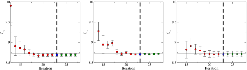
Figure 1: (Color online) Comparison between three different criteria to assess the convergence of the density of states, for the specific heat $C_{V}$ at $\beta=0.316$. The horizontal line is the central value obtained with the Morozov-Lin criterion (middle plot) at the 27th iteration. The left plot has been obtained with the Wang-Landau flat histogram method, while the right plot shows the data obtained with the Zhou-Bhatt criterion. The vertical line marks the 23rd iteration.

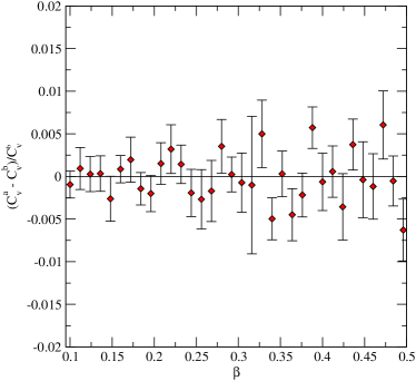
Figure 2: (Color online) The difference between the specific heat determined with the Zhou-Bhatt ($C_{V}^{a}$) and the Morozov-Lin criterion ($C_{V}^{b}$) divided by $C_{V}^{b}$ (both taken after 23 iterations), on a wide range of $\beta$ for the $16^{3}$ lattice.

In Fig. 1, we provide a comparison of the flat histogram criterion, the criterion proposed in Zhou:2005aa and the criterion introduced in Morozov:2007 for the specific heat

$$C=\frac{\beta^{2}}{L^{3}}\left(\big{\langle}E^{2}\big{\rangle}-\big{\langle}E\big{\rangle}^{2}\right)$$ (7)

at $\beta=0.316$ on a $16^{3}$ lattice. The figure shows that after 20 iterations all the three criteria are at convergence. Moreover, the three estimates for the specific heat are the same within errors, the typical size of the errors being a few percent. This general feature is independent from $\beta$. An explicit comparison of the Zhou-Bhatt criterion with the Morozov-Lin criterion focusing again on the specific heat is provided in Fig. 2 for a wide range of $\beta$. This suggests that for observables that are accurate to the level of the percent, among which are interface tensions, the three criteria yield compatible results. In terms of statistical errors, the Zhou-Bhatt criterion seems to yield the largest error bars. However, the Zhou-Bhatt algorithm converges to the density of the states in a CPU time that is a factor of 16 smaller than the original Wang-Landau and a factor of 64 smaller than the Morozov-Lin criterion. This study suggests that for our application the Zhou-Bhat criterion (i.e. number of visits $\propto 1/\sqrt{\log k}$) is adequate from the numerical point of view for the level of precision requested by our study. Hence, we used this criterion to decide when a given iteration had converged. Based on the study of Fig. 1, we performed 23 iterations, which is a conservative estimate of the number of iterations needed for the convergence of the algorithm.

To perform further tests of our implementation, we calculated some thermodynamical quantities like the critical temperature, the latent heat and the entropy density, and compared our results with Refs. MartinMayor:2006gx ; Bazavov:2008qg . Following Bazavov:2008qg , we use three different estimators for the transition temperature on lattices with finite extension. The first, $\beta^{1}_{c}$, is defined to be the value for which the canonical distribution $P(E,\beta)=g(E)e^{-\beta E}$ has two equal maxima. The second ($\beta^{2}_{c}$) is the position of the central energy of the latent heath, i.e. the value of $\beta$ satisfying the equation

$$e(\beta^{2}_{c})=\frac{1}{2}\left[e^{+}(\beta^{2})+e^{-}(\beta^{2})\right]\ ,$$ (8)

where $e^{\pm}$ ($e=E/N$, with $N=L^{3}$) are the locations of the maxima of the probability distribution at $\beta_{c}^{2}$. The third ($\beta^{3}_{c}$) is the location of the maximum of the specific heat 7. All the critical temperatures are extrapolated to the infinite volume limit using the ansatz

$$\beta^{i}_{c}(L)=\beta^{i}_{c}+\frac{c^{i}}{L^{3}}\ .$$ (9)

We perform the extrapolation by using the six largest lattices. The extrapolated values agree in the infinite-volume limit (see Fig. 3). Averaging over the three determinations gives $\beta_{c}=0.3143103(9)$.

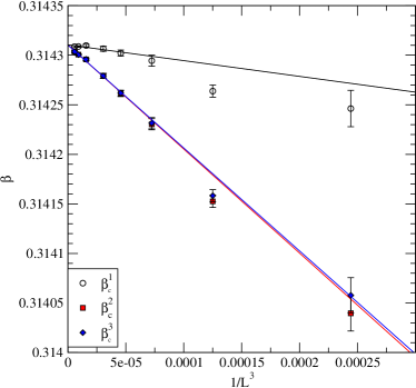
Figure 3: (Color online) Three different estimators for the critical temperature on finite lattices.

The latent heat per site $\Delta e$ can be calculated from the maxima of the specific heat Challa:1986sk :

$$C_{\rm max}(L)=c+\frac{1}{4}(\beta_{c})^{2}(\Delta e)^{2}L^{3}\ .$$ (10)

Our estimate is $\Delta e=1.16454(16)$. Finally, the numerically determined entropy density

$$s=\beta(e-f)\ ,$$ (11)

with $f=-\log Z/(\beta N)$ the free energy density, is plotted in Fig. 4.

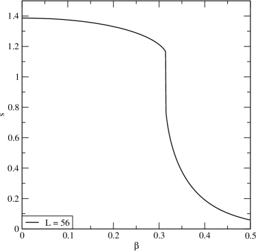
Figure 4: Entropy density as a function of $\beta$ for $L=56$.

All those quantities are always less than two standard deviations from the corresponding determinations of MartinMayor:2006gx , which have been obtained on larger lattices.

IV Interface tensions

We now move to the discussion of our results for the interface tension. In the ordered phase, an interface can form between two regions of space that are in two different vacua. This interface is called the order-oder interface. Near the critical temperature, the dynamics of the order-order interface $\sigma_{oo}$ is dominated by massless modes and its infrared properties are universal (see e.g. Luscher:1980fr ; Privman:1992zv ). The asymptotic interface tension can then be extracted using the ansatz (see e.g. billo:2006zg ; Caselle:2007yc )

$$\sigma_{oo}(L)=\sigma_{oo}+\frac{c_{2}}{L^{2}}+\frac{c_{4}}{L^{4}}+\dots\ ,$$ (12)

where the order of the truncation of the expansion in $1/L^{2}$ is determined by the accuracy of the data. As a consequence, a reliable extraction of $\sigma$ requires accurate data. From our simulations, we have extracted $F_{I}$ using Eq. (1) and then the interface tension fitting the data according to Eq. (12) truncated to ${\cal O}(L^{-4})$. To reduce finite size effects, we included in the fit only points for which $L\sqrt{\sigma}\geq 6$. Since the ansatz (12) is expected to hold only at large distances, our analysis was limited to values of $\beta$ for which $\sigma_{oo}^{-1/2}\geq 3$. An example of the quality of our data is given in Fig. 5.

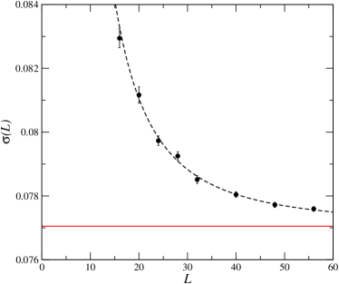
Figure 5: (Color online) The order-order interface tension $\sigma(L)$ at $\beta=0.318$ for different lattice sizes. The dashed line is a fit of the data according to Eq. (12), with fit parameters $\sigma_{oo}$, $c_{2}$ and $c_{4}$; the horizontal line indicates the extracted value for $\sigma_{oo}$.

The values of $\sigma_{oo}$ extracted from our fits are plotted in Fig. 6. The relative error on this quantity is at most $3\times 10^{-3}$, and is invisible on the scale of the figure. Near $\beta_{c}$, the behavior of $\sigma_{oo}(\beta)$ can be parametrized as

$$\sigma_{oo}(\beta)=\sigma_{oo}(\beta_{c})+a\left(\beta-\beta_{c}\right)^{\rho}\ .$$ (13)

Fitting this functional form to our results, we found that this provides an excellent description of the data (a fit with 9 degrees of freedom has $\chi^{2}/9=0.11$). We find $\sigma_{oo}(\beta_{c})=0.0249(6)$ and $\rho=0.76(4)$. The quality of the fit is shown by the dashed line in Fig. 6.

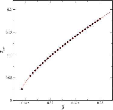
Figure 6: (Color online) The infinite volume order-order interface tension as a function of $\beta$. The fit (dashed line) is in excellent agreement with the hypothesis of perfect wetting (open triangle).

At $\beta_{c}$, the order-disorder interface separates a region in an ordered state from one in the disordered state. The interface tension between an ordered and the disordered phase, $\sigma_{od}$, can be determined by looking at the probability distribution of the energy at the critical temperature. In particular, if $P_{\rm max}$ is the peak of the histogram when the two maxima have equal eight and $P_{\rm min}$ is the minimal height of the valley between the two peaks Lee:1990ti ; Berg:1992qua ,

$$2\sigma_{\rm od}(L)=\frac{1}{L^{2}}\log\left(\frac{P_{\rm max}}{P_{\rm min}}\right)\ .$$ (14)

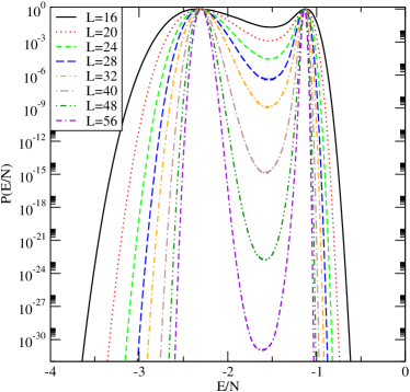
Figure 7: (Color online) The probability distribution at the critical temperature. The maxima are normalized to one.

Our data for $P(E/N)$ as a function of $E/N$ are shown in Fig. 7. We use a fitting function of the form

$$2\sigma_{\rm od}(L)=-\frac{\log L}{2L^{2}}+2\sigma_{\rm od}+\frac{c_{2}}{L^{2}}+\frac{c_{3}}{L^{3}}+\frac{c_{4}}{L^{4}}\ .$$ (15)

Universality arguments Luscher:2004ib ; Aharony:2009gg suggest that $c_{3}=0$. Nevertheless, a correction at this order is due to the fact that we use the finite-volume estimator (14), as it can be shown with a simple saddle point argument . A fit of the data according to Eq. (15) performed excluding the two smallest volumes yields $2\sigma_{\rm od}=0.0252(4)$, with $c_{3}$ and $c_{4}$ both compatible with zero. Note that the obtained value of $\sigma_{\rm od}$ is fully compatible with the perfect wetting relationship

$$2\sigma_{\rm od}=\sigma_{\rm oo}\ ,$$ (16)

which has been argued in Borgs:1992qd for the two-dimensional Potts model. Our result is a clear indication that perfect wetting also holds for the Potts model in three dimensions. This is shown in Fig. 6.

V Conclusions

We have proposed a method for determining numerically free energies of interfaces or topological objects when the partition function with given boundary conditions is required. The range of applicability of our method includes not only statistical systems ($XY$ model, Heisenberg ferromagnet etc.), but also gauge theories (e.g. the ’t Hooft loop tension in SU($N$) Yang-Mills). We have successfully tested this method on the 3D four-state Potts model, for which we have provided a very accurate determination of the order-order interface below the critical temperature. This has enabled us to give clear numerical evidence for perfect wetting in this model.

References

- (1) V. Privman, Int.J.Mod.Phys. C3, 857 (1992), arXiv:cond-mat/9207003.
- (2) T. Goto, Prog.Theor.Phys. 46, 1560 (1971).
- (3) Y. Nambu, Phys.Rev. D10, 4262 (1974).
- (4) P. de Forcrand, M. D’Elia, and M. Pepe, Phys.Rev.Lett. 86, 1438 (2001), arXiv:hep-lat/0007034.
- (5) P. de Forcrand, B. Lucini, and D. Noth, PoS LAT2005, 323 (2006), arXiv:hep-lat/0510081.
- (6) K. Kajantie and L. Karkkainen, Phys.Lett. B214, 595 (1988).
- (7) K. Kajantie, L. Karkkainen, and K. Rummukainen, Phys.Lett. B223, 213 (1989).
- (8) C. Korthals Altes, A. Michels, M. A. Stephanov, and M. Teper, Phys.Rev. D55, 1047 (1997), arXiv:hep-lat/9606021.
- (9) F. Wang and D. P. Landau, Phys. Rev. Lett. 86, 2050 (2001).
- (10) C. Zhou and R. N. Bhatt, Phys. Rev. E72, 025701 (2005).
- (11) Q. Yan and J. de Pablo, Phys. Rev. Lett. 90, 035701 (2003).
- (12) R. Belardinelli and V. Pereyra, J.Chem.Phys. 127, 184105 (2007).
- (13) A. Morozov and S. Lin, Phys. Rev. E 76, 026701 (2007).
- (14) A. Morozov and S. Lin, J.Chem.Phys. 130, 074903 (2009).
- (15) V. Martin-Mayor, Phys. Rev. Lett. 98, 137207 (2007), arXiv:cond-mat/0611543.
- (16) A. Bazavov, B. A. Berg, and S. Dubey, Nucl.Phys. B802, 421 (2008), arXiv:0804.1402.
- (17) M. S. Challa, D. Landau, and K. Binder, Phys.Rev. B34, 1841 (1986).
- (18) M. Luscher, K. Symanzik, and P. Weisz, Nucl.Phys. B173, 365 (1980).
- (19) M. Billò, M. Caselle, and L. Ferro, JHEP 0602, 070 (2006), arXiv:hep-th/0601191.
- (20) M. Caselle, M. Hasenbusch, and M. Panero, JHEP 09, 117 (2007), arXiv:0707.0055.
- (21) J. Lee and J. Kosterlitz, Phys.Rev.Lett. 65, 137 (1990).
- (22) B. Berg and T. Neuhaus, Phys.Rev.Lett. 68, 9 (1992), arXiv:hep-lat/9202004.
- (23) M. Luscher and P. Weisz, JHEP 0407, 014 (2004), arXiv:hep-th/0406205.
- (24) O. Aharony and E. Karzbrun, JHEP 0906, 012 (2009), arXiv:0903.1927.
- (25) C. Borgs and W. Janke, J.Phys.IFrance 2, 2011 (1992).