Weighted algorithms for compressed sensing and matrix completion

Abstract

This paper is about iteratively reweighted basis-pursuit algorithms for compressed sensing and matrix completion problems. In a first part, we give a theoretical explanation of the fact that reweighted basis pursuit can improve a lot upon basis pursuit for exact recovery in compressed sensing. We exhibit a condition that links the accuracy of the weights to the RIP and incoherency constants, which ensures exact recovery. In a second part, we introduce a new algorithm for matrix completion, based on the idea of iterative reweighting. Since a weighted nuclear “norm” is typically non-convex, it cannot be used easily as an objective function. So, we define a new estimator based on a fixed-point equation. We give empirical evidences of the fact that this new algorithm leads to strong improvements over nuclear norm minimization on simulated and real matrix completion problems.

Keywords. Compressed Sensing; Weighted Basis-Pursuit; Matrix Completion

1 Introduction

In this paper, we consider the statistical analysis of high dimensional structured data in two close setups: vectors with small support and matrices with low rank. In the first setup, known as Compressed Sensing (CS) [20, 15, 7, 6, 21, 9], the aim is to reconstruct a high dimensional vector with only few non-zero coefficients, based on a small number of linear measurements. In the second setup, called Matrix Completion [10, 23, 5, 26], we aim at reconstructing a small rank matrix from the observations of only a few entries. Both problems are motivated by many practical applications in many different domains (medical [22], imaging [12], seismology [16], recommending systems such as the Netflix Prize, etc.) as well as theoretical challenges in many different fields of mathematics (random matrices, geometry of Banach spaces, harmonic analysis, empirical processes theory, etc.). From an algorithmic viewpoint, one central idea is the convex relaxation of the $\ell_{0}$-functional (the function giving the number of non-zero coefficients of a vector) and of the rank function. This idea gave birth to two well-known algorithms: the Basis Pursuit algorithm [15]  and nuclear norm minimization [5]. Many results have been obtained for these two algorithms and we refer the reader to the next sections for more details. Here we will be interested in weighted versions of these algorithms, see [11] in the CS setup. In particular, we will be interested in finding theoretical explanation underlying the fact that, empirically, it is observed that weighted Basis pursuit outperforms classical Basis Pursuit. We will also propose a way to export the idea of reweighting into the Matrix Completion problem.

2 Weighted basis-pursuit in Compressed Sensing

One way of setting the CS problem is to ask the following question. Starting with a $m\times N$ matrix $A$, called a sensing or measurement matrix, and with a vector $x$ in $\mathbb{R}^{N}$, is it possible to reconstruct $x$ from the linear measurements $Ax$? Classical linear algebra theory tells that we need at least $m\geq N$ to recover $x$ from $Ax$ in order to find a unique solution to the linear system. But, if more is known on $x$, then, hopefully, a smaller number $m$ of measurements may be enough.

In the theory of CS, it is now well-understood that it is indeed possible to recover sparse signals (signals with a small support, the support being the set of non-zeros entries) from a small number of linear measurements. If $x$ is a sparse vector and $A$ a “good” measurement matrix (in a sense to be clarified later), then looking for a vector $y$ with the smallest support and satisfying $Ay=Ax$ can recover $x$ exactly. This procedure, called the $\ell_{0}$ or support minimization procedure, is known to be the best theoretical procedure to recover any $s$-sparse vector $x$ (vectors with a support size smaller than $s$) from $Ax$ as long as $A$ is injective on the set of all $s$-sparse vectors. However, this problem is NP-hard, and alternatives are suitable in practice, in part because the function $x\mapsto|x|_{0}$ ($|x|_{0}$ stands for the cardinality of the support of $x$) is not convex.

A natural remedy to this problem is convex relaxation. In [15], the authors propose to minimize the $\ell_{1}$-norm as the convex envelope of this non-convex function, leading to the so-called Basis-Pursuit algorithm (BP). The BP algorithm minimizes the $\ell_{1}$ norm on the affine space $x+\ker A$. Namely, consider, for any $y\in\mathbb{R}^{m}$:

$$\Delta_{1}(y)\in\operatorname*{argmin}_{t\in\mathbb{R}^{N}}\Big{(}|t|_{1}:At=y\Big{)},$$ (2.1)

so that $\Delta_{1}(Ax)$ is a candidate for the reconstruction of $x$ based on $Ax$. We say that $x$ is exactly reconstructed by $\Delta_{1}$, namely $\Delta_{1}(Ax)=x$, when $x$ is the unique solution of the minimization problem (2.1) when $y=Ax$.

Note that other algorithms have been introduced in the CS literature. For instance, $\ell_{p}$-minimization algorithms for $0<p<1$ are considered in [13, 24, 46, 14]. Some greedy algorithms based on the ideas of the Matching Pursuit algorithm of [19, 35] have been used in CS, see [38, 39, 49] for instance.

In the present paper, we consider weighted-$\ell_{1}$ minimization over $x+\ker A$. This algorithm was introduced in [11]. Since then, it has drawn a particular attention because it is now acknowledged, although mainly only empirically observed, that a proper weighted basis-pursuit algorithm can improve a lot upon basic basis-pursuit. This is illustrated in Figure 1, and many other numerical experiments can be found in [11]. However, theoretical explanations of this fact are still lacking. Some results that go in this direction are given in [31, 51, 32], [14], [31]. But, the results given in these papers are of a different nature than ours, since they are using a random model for the unknown vector $x$, such as a vector with i.i.d $N(0,1)$ non-zero entries, with a distribution support which is uniform conditionally on the sparsity. In the statement of our results, $x$ is an arbitrary deterministic sparse vector. In [18] an iteratively reweighted least-squares procedure is studied, as an approximation of basis-pursuit.

We introduce the weighted algorithm: for any $y\in\mathbb{R}^{m}$ and any sequence $w=(w_{1},\ldots,w_{N})\in\mathbb{R}^{N}$ of non-negative weights,

$$\Delta_{w}(y)\in\operatorname*{argmin}_{t\in\mathbb{R}^{N}}\Big{(}\sum_{i=1}^{N}\frac{|t_{i}|}{w_{i}}:At=y\Big{)}.$$ (2.2)

We use the convention $t/0=\infty$ when $t>0$ and $0/0=0$. Note that, under this convention, the algorithm (2.2) is defined according to the support $I_{w}$ of $w$ by

$$\big{(}\Delta_{w}(y)\big{)}_{I_{w}^{c}}=0\;\text{ and }\;\big{(}\Delta_{w}(y)\big{)}_{I_{w}}\in\operatorname*{argmin}_{t\in\mathbb{R}^{I_{w}}}\Big{(}\sum_{i\in I_{w}}\frac{|t_{i}|}{w_{i}}:A_{I_{w}}t=y\Big{)},$$ (2.3)

where if $t\in\mathbb{R}^{N}$ and $I\subset\{1,\ldots,N\}$, we denote by $t_{I}$ the vector such that $(t_{I})_{i}=t_{i}$ if $i\in I$ and $(t_{I})_{i}=0$ if $i\notin I$. Once again, we say that $x$ is exactly reconstructed by $\Delta_{w}$, namely $\Delta_{w}(Ax)=x$, when $x$ is the unique solution of the minimization problem (2.2) when $y=Ax$. In particular, this requires that the support of $x$ is included in the support of $w$.

2.1 No-loss property

Note that when the weight vector $w$ is close to $x$, then $\sum_{i=1}^{N}|x_{i}|/w_{i}$ is close to $|x|_{0}$. Moreover, for “reasonable” matrices $A$, the vector $x$ is the one with the shortest support in the affine space $x+\ker A$. So, a natural choice for $w$ in (2.2) is $w=|\Delta_{1}(Ax)|$. We denote this decoder by $\Delta_{2}$:

$$\Delta_{2}(y)\in\operatorname*{argmin}_{t\in\mathbb{R}^{N}}\Big{(}\sum_{i=1}^{N}\frac{|t_{i}|}{|\Delta_{1}(y)_{i}|}:At=y\Big{)}.$$ (2.4)

The next Theorem proves that $\Delta_{2}$ is at least as good as the Basis Pursuit algorithm $\Delta_{1}$.

Theorem 1.

Let $x\in\mathbb{R}^{N}$. If $\Delta_{1}(Ax)=x$, then $\Delta_{2}(Ax)=x$.

The proof of Theorem 1 is based on the well-known null space property and dual characterization of [6], see Section 4 below. However, it was observed empirically in [11] that it is better to consider positive weights, and thus, to consider, for some $\varepsilon>0$, the weights $w_{i}=|\Delta_{1}(y)_{i}|+\varepsilon$ for $i=1,\ldots,N$. This is easily understood: if for some $i\in\{1,\ldots,N\}$, $\Delta_{1}(Ax)_{i}=0$ while $x_{i}\neq 0$, then $\Delta_{2}(Ax)_{i}$ is also equal to $0$ and there is no hope to recover $x$ using $\Delta_{2}$ as well. By adding an extra $\varepsilon$ term to each weights, the necessary support condition $\operatorname{supp}(x)\subset\operatorname{supp}(w)$ to reconstruct $x$ from $\Delta_{w}(Ax)$ is satisfied (see for instance Proposition 1 in Section 4). The choice of $\varepsilon>0$ can be done in a data-driven way, see [11].

2.2 An empirical evidence

In Figure 1, we give a simple illustration of the fact that weighted basis-pursuit can improve a lot upon basic basis-pursuit, using a simple numerical experiment. For many combinations of $m$ ($y$-axis) and $s$ ($x$-axis), we repeat the following experiment 50 times: draw at random a sensing matrix $A$ with i.i.d $N(0,1/m)$ entries and draw at random a vector with $s$ non-zero coordinates chosen uniformly, with i.i.d $N(0,1)$ non-zero entries. Then, compute $\hat{x}_{1}=\Delta_{1}(Ax)$ and $\hat{x}_{w}=\Delta_{20}^{\varepsilon}(Ax)$ (here we take $\varepsilon=0.01$ without further investigation), where $\Delta_{k}^{\varepsilon}(Ax)$ is computed iteratively, using

$$\Delta_{k+1}^{\varepsilon}(Ax)\in\operatorname*{argmin}_{t\in\mathbb{R}^{N}}\Big{(}\sum_{i=1}^{N}\frac{|t_{i}|}{|\Delta_{k}^{\varepsilon}(Ax)_{i}|+\varepsilon}:At=Ax\Big{)}.$$ (2.5)

Then, we count the number of exact reconstructions achieved by $\hat{x}_{1}$ and $\hat{x}_{w}$ over the 50 repetitions. The plots on the left are the exact recovery counts of $\hat{x}_{1}$ (black means exact recovery over the 50 repetitions) while the plots on the right are the exact recovery counts of $\hat{x}_{w}$. In these figures, exact recovery is declared exact when $|\hat{x}-x|_{2}/|x|_{2}<\eta$, where we take $\eta=10^{-5}$ on the first line and $\eta=10^{-6}$ on the second line. The red curve is a theoretical “phase-transition” threshold $s\mapsto s\log(em/s)$. We observe in these figures that $\hat{x}_{w}$ improves a lot upon $\hat{x}_{1}$, in particular when $\eta=10^{-6}$.

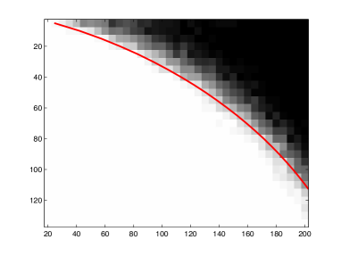
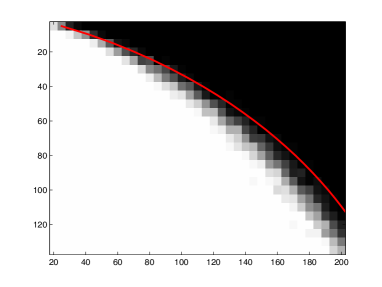
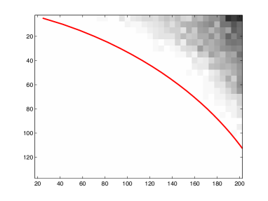
Figure 1: Exact recovery counts (black means exact recovery) of basis-pursuit (left column) and weighted basis-pursuit (right column), where the $x$-axis is the sparsity ($s$) and the $y$-axis is the number of measurements ($m$). Exact recovery is declared with a tolerance equal to $10^{-5}$ on the first line, and equal to $10^{-6}$ on the second line. The red curve is a theoretical phase-transition threshold $s\mapsto s\log(em/s)$

2.3 A theoretical explanation

Now, we want to understand if $\Delta_{2}$ can do better than $\Delta_{1}$, and why. In particular, if $\Delta_{1}(Ax)$ is close to $x$ (but fails to reconstruct exactly $x$), under which condition do we get $\Delta_{2}(Ax)=x$? In general, given a weight vector $w\in\mathbb{R}^{N}$, what conditions on $w$ can insure that $\Delta_{w}(Ax)=x$? In Theorem 2 below, we use the duality argument of [6] to prove that the condition

$$(A0)(I,C)\hskip 28.45274pt|w_{I^{c}}|_{\infty}\big{|}(1/w)_{I}\big{|}_{2}\leq C,$$ (2.6)

where $I$ is the support of $x$ and $C\geq 0$ is such that

$$C\leq\frac{1-\delta}{\mu},$$

where $\delta$ and $\mu$ are, respectively, the restricted isometry and incoherency constants [8, 6, 7] of the matrix $A$, ensure that the $w$-weighted algorithm $\Delta_{w}$ recovers exactly $x$ given $Ax$.

It is interesting to note that, so far, only random matrices are able to satisfy the incoherency and isometry properties for small values of $m$. Thus, if one wants the number $m$ of measurements to be of the order (up to some logarithmic factor) of the sparsity of the vector to recover, one has to consider random matrices. This leads to results in Compressed Sensing that hold with a large probability, with respect to the randomness involved in the construction of the sensing matrix. In practice, however, the most interesting sensing matrices are structured matrices, like the Fourier or the Walsh matrices (see [8, 45]), since these matrices can be stored and constructed by efficient algorithms. A lot of research go in this direction, and we don’t consider this problem here, but rather focus on weighted algorithms. Therefore, we will state our probabilistic results for a simple (and somehow universal) sensing matrix $A$ with entries being i.i.d. centered Gaussian variables with variance $1/m$.

Theorem 2.

Let $x\in\mathbb{R}^{N}$ and denote by $I$ its support and by $s$ the cardinality of $I$. Let $C,\mu>0$ and $0<\delta<1$. Assume that

$$m\geq c_{0}\max\Big{[}\frac{s}{\delta^{2}},\frac{s\log N}{\mu^{2}}\Big{]}\;\mbox{ and }\;C\leq\frac{1-\delta}{\mu},$$

where $c_{0}$ is a purely numerical constant. Consider the event $\Omega(I,C)=\{|w_{I^{c}}|_{\infty}\big{|}(1/w)_{I}\big{|}_{2}\leq C\}$ and let $A$ be a $m\times N$ matrix with entries being i.i.d. centered Gaussian random variables with variance $1/m$. Then, with probability larger than

$$1-2\exp(-c_{1}m\delta^{2})-\exp\big{(}-c_{2}\mu^{2}m/s\big{)}-\mathbb{P}\Big{[}\Omega(I,C)^{\complement}\Big{]},$$

the vector $x$ is exactly reconstructed by $\Delta_{w}(Ax)$.

Theorem 2 gives an explicit condition, linking the incoherency constant $\mu$, the restricted isometry constant $\delta$, and the constant $C$ from condition $A0(I,C)$ on the weights $w$ that ensures the exact reconstruction of $x$ using $\Delta_{w}$. This is the first result of this nature for weighted basis pursuit.

When $w_{I^{c}}=0$ then $(A0)(I,C)$ holds with $C=0$, so that one can take $\delta=1$ and $\mu=+\infty$. This is the case for $w=(|\Delta_{1}(Ax)_{i}|)_{i=1}^{N}$ when $\Delta_{1}(Ax)=x$. This condition is also satisfied when the weights vector $w$ is close enough to $|x|$ and when the absolute value of the non-zero coordinates of $|x|$ are sufficiently large. For instance, $(A0)(I,C)$ holds when

$$\min_{i\in I}|x_{i}|\geq\Big{(}1+\frac{\sqrt{|I|}}{C}\Big{)}|w-|x||_{\infty}.$$ (2.7)

Indeed, if we denote $\varepsilon=|w-|x||_{\infty}$ then $(A0)(I,C)$ follows from (2.7) since $\max_{i\in I^{c}}w_{i}\leq\varepsilon$ and

$$\Big{|}\Big{(}\frac{1}{w}\Big{)}_{I}\Big{|}\leq\frac{\sqrt{|I|}}{\min_{i\in I}w_{i}}\leq\frac{\sqrt{|I|}}{\min_{i\in I}|x_{i}|-\varepsilon}.$$

In particular, if $A0(I,C)$ is satisfied with $C=c_{1}/\sqrt{\log N}$, for some constant $0<c_{1}<1$, then a proportional to $s$ number of Gaussian measurements will be enough to get $\Delta_{w}(Ax)=x$ with a large probability.

In Figure 2 below, we give an empirical illustration of the fact that $A0(I,C)$ is indeed a relevant condition for exact reconstruction of weighted basis-pursuit. We consider exactly the same experiment as what we did in Section 2.2, but this time we fix the number of measurements to $m=110$ and the sparsity of $x$ to $s=45$. For this combination of $m$ and $s$, the phase transition occurs, namely basis pursuit can either work or not, see Figure 1, so we can expect for these values a strong improvement of weighted basis-pursuit over non-weighted one. On the left-side of Figure 2, we show the value of the constant $C$ over the reweighting iterations. Namely, if $I$ is the support of the true unknown vector $x$, we compute for $k=1,\ldots,K$ the values of

$$C^{k}=|w_{I^{c}}^{(k)}|_{\infty}\big{|}(1/w^{(k)})_{I}\big{|}_{2},$$

where

$$w^{(k)}=|\Delta_{k}^{\varepsilon}(Ax)|+\varepsilon$$

over the 10 repetitions (differentiated by different colors), where we recall that $\Delta_{k}^{\varepsilon}(Ax)$ is given by (2.5) and where we choose $K=30$. On the right-side of Figure 2, we show the logarithm of relative reconstruction errors over the iterations, namely

$$\mathrm{err_{k}}=\log\Big{(}\frac{|\Delta_{k}^{\varepsilon}(Ax)-x|_{2}}{|x|_{2}}\Big{)}$$

(we take the logarithm only for illustrational purpose, so that we can see the cases when exact reconstructions occurs). Each repetition of the experiment is represented with a different color.

What we observe is a direct correspondence between the constant $C$ from Assumption $A0(I,C)$ and the quality of reconstruction of weighted basis pursuit along the iterations. This tells that Assumption $A0(I,C)$ indeed explains (at least in the considered configuration) when exact reconstruction can or cannot happen using weighted basis pursuit.

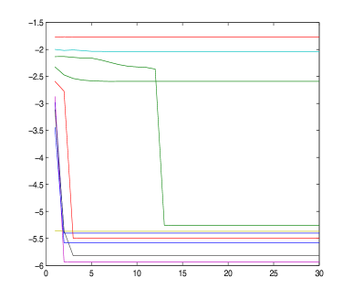
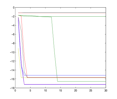
Figure 2: Logarithm of the value of the constant $C$ from Assumption $A0(I,C)$ (left) and logarithm of the relative reconstruction error of weighted basis pursuit over the iterations (right).

Remark 1.

Note that uniform results can also be derived for the weighted-$\ell_{1}$ algorithm. Indeed, by using classical machinery, it can be proved that 1) implies 2) implies 3) where:

1. for all $x\in\Sigma_{s}$, $A\operatorname{diag}(w)$ satisfies $\mathrm{RIP}(\delta,8s)$ and $I_{x}\subset I_{w}$,

2. $\sup_{x\in\ker(A\operatorname{diag}(w))\cap B_{1}^{N}}\left|x\right|_{2}<\frac{1}{2\sqrt{s}}$ and $\forall x\in\Sigma_{s},I_{x}\subset I_{w}$,

3. for any $x\in\Sigma_{s},\Delta_{w}(Ax)=x$.

But, it is not clear why, for instance when $w=\Delta_{1}(Ax)$, it would be easier for the matrix $A\operatorname{diag}(\Delta_{1}(Ax))$ to satisfy $\mathrm{RIP}$ than for $A$ itself. The same remark also holds for the euclidean section of $B_{1}^{N}$ by the kernel of $A\operatorname{diag}(\Delta_{1}(Ax))$ or $A$. These approaches look too crude to perform a study of $\ell_{1}$-weighted algorithms, where most of the gain can be done only on the absolute multiplying constant in front of the minimal number of measurements $m$ needed for exact reconstruction.

2.4 Verifying exact reconstruction

Thanks to Theorem 1, it is easy to test if we were able to reconstruct exactly a vector $x$ given $Ax$. So far, we have to rely on the theory to insure that with a high probability, we have $\Delta_{1}(Ax)=x$. Using (2.4), we can verify this belief. Indeed, Theorem 1 entails that $\Delta_{2}(Ax)=x$ when $\Delta_{1}(Ax)=x$. In particular, if $\Delta_{1}(Ax)\neq\Delta_{2}(Ax)$, then we are sure that we didn’t perform the exact reconstruction of $x$ using $\Delta_{1}(Ax)$. Then, we can iterate the mechanism and define for any $k\geq 1$

$$\Delta_{k+1}(Ax)\in\operatorname*{argmin}_{t\in\mathbb{R}^{N}}\Big{(}\sum_{i=1}^{N}\frac{|t_{i}|}{|\Delta_{k}(Ax)_{i}|}:At=Ax\Big{)},$$

leading to a sequence

$$\Delta_{1}(Ax),\Delta_{2}(Ax),\cdots,\Delta_{r}(Ax).$$ (2.8)

If the sequence (2.8) does not become constant after a certain number of iterations, then it is very likely that none of the algorithm $\Delta_{k}(Ax)$ reconstructed exactly $x$. We also have the following reverse statement. Denote by $\Sigma_{k}$ the set of all $k$-sparse vectors in $\mathbb{R}^{N}$.

Theorem 3.

Let $A$ be a $m\times N$ injective matrix on $\Sigma_{m}$ and let $x\in\Sigma_{\lfloor m/2\rfloor}$. The following statements are equivalent:

1. There exists an integer $r$ such that $\Delta_{r}(Ax)=x$,

2. The sequence $\Delta_{1}(Ax),\Delta_{2}(Ax),\ldots,$ becomes constantly equal to a $\lfloor m/2\rfloor$-sparse vector after a certain number of iterations.

Note that the matrix with i.i.d. standard Gaussian entries is injective on $\Sigma_{m}$ with probability one. Thus, we propose to compute the sequence (2.8) as an empirical test for the exact reconstruction of a vector $x$ from $Ax$.

3 Iteratively weighted soft-thresholding for matrix completion

In many applications, data can be represented as a database with missing entries. The problem is then to fill the missing values of the database, leading to the so-called matrix completion problem. For instance, collaborative filtering aims at doing automatic predictions of the taste of users, using the collected tastes of every users at the same time [25]. The popular Netflix prize is a popular application of this problem. Other applications include machine-learning [1], control [37], quantum state tomography [27], structure from motion [48], among many others. This problem can be understood as a non-commutative extension of the compressed sensing problem. So, a natural question is the following: Does the principle of iterative weighting of the $\ell_{1}$-norm work also for matrix completion? In this Section, we prove empirically that the answer to this question is yes. We prove that one can improve the convex relaxation principle for matrices, which is based on the nuclear norm [10], [26], by using a weighted nuclear norm, in the same way as we did for vectors in Section 2. However, note that there is, as explained below, a major difference between the vectors and matrices cases at this point, since a weighted nuclear norm is not convex in general, while a weighted $\ell_{1}$-norm is.

Let us first recall standard definitions and notations. Let $A_{0}\in\mathbb{R}^{n_{1}\times n_{2}}$ be a matrix with $n_{1}$ rows and $n_{2}$ columns. The matrix $A_{0}$ is not fully observed. What we observe is a given subset $\Omega\subset\{1,\ldots,n_{1}\}\times\{1,\ldots,n_{2}\}$ of cardinality $m$ of the entries of $A_{0}$, where $m\ll n_{1}n_{2}$. For any matrix $A\in\mathbb{R}^{n_{1}\times n_{2}}$, we define the masking operator ${\mathcal{P}}_{\Omega}(A)\in\mathbb{R}^{n_{1}\times n_{2}}$ such that $({\mathcal{P}}_{\Omega}(A))_{j,k}=A_{j,k}$ when $(j,k)\in\Omega$ and $({\mathcal{P}}_{\Omega}(A))_{j,k}=0$ when $(j,k)\notin\Omega$. We define also ${\mathcal{P}}_{\Omega}^{\perp}(A)=A-{\mathcal{P}}_{\Omega}(A)$.

Since we consider the case where $m\ll n_{1}n_{2}$, the matrix completion problem is in general severely ill-posed. So, one needs to impose a complexity or sparsity assumption on the unknown matrix $A_{0}$. This is done by assuming that $A_{0}$ has low rank, which is the natural extension of the sparsity assumption for vectors to the spectrum of a matrix. For the problem of exact reconstruction, other geometrical assumptions are necessary (such as the incoherency assumption, see [5, 10, 31]). Under such assumptions, it is now well-understood that the principle of convex relaxation of the rank function is able to reconstruct exactly the unknown matrix from few measurements, see [5, 10, 26, 43]. Indeed, a natural approach would be to solve the problem

$$\begin{split}&\text{ minimize }\operatorname*{rank}{A}\\ &\text{ subject to }{\mathcal{P}}_{\Omega}(A)={\mathcal{P}}_{\Omega}(A_{0}),\end{split}$$ (3.1)

but this minimization problem is known to be very hard to solve in practice even for small matrices, see for instance [5, 10]. The convex envelope of the rank function over the unit ball of the operator norm is the nuclear norm, see [23], which is given by

$$\|A\|_{1}=\sum_{j=1}^{n_{1}\wedge n_{2}}\sigma_{j}(A),$$

(it is the bi-conjugate of the rank function over the unit ball of the operator norm), where $\sigma_{1}(A)\geq\cdots\geq\sigma_{n_{1}\wedge n_{2}}(A)$ are the singular values of $A$ in decreasing order. So, the convex relaxation of (3.1) is

$$\begin{split}&\text{ minimize }\|A\|_{1}\\ &\text{ subject to }{\mathcal{P}}_{\Omega}(A)={\mathcal{P}}_{\Omega}(A_{0}).\end{split}$$ (3.2)

This problem has received a lot of attention quite recently, see [5, 10, 26, 30, 43], among many others. The point is that, in the same way as the basis pursuit for vectors, (3.2) is able to recover exactly $A_{0}$ with a large probability, based on an almost minimal number of samples (under some geometrical assumption).

In literature concerned about computational problems [34], [36], [47, 33], among others, the relaxed version of (3.2) is considered, since it is easier to construct a solver for it (one can apply generic first-order optimal methods, such as proximal forward-backward splitting [17], among many other methods) and since it is more stable in the presence of noise. Note that the SVT algorithm of [4] gives a solution under equality constraints for an objective function with an extra ridge term $\|A\|_{1}+\tau\|A\|_{2}^{2}$. The relaxed problem is simply formulated as penalized least-squares:

$$\hat{A}_{\lambda}\in\operatorname*{argmin}_{A\in\mathbb{R}^{n_{1}\times n_{2}}}\Big{\{}\frac{1}{2}\|{\mathcal{P}}_{\Omega}(A)-{\mathcal{P}}_{\Omega}(A_{0})\|_{2}^{2}+\lambda\|A\|_{1}\Big{\}},$$ (3.3)

where $\lambda>0$ is a parameter balancing goodness-of-fit and complexity, measured by the nuclear norm.

Before we go on, we need some notations. The vector of singular values of $A$ is denoted by $\sigma(A)=(\sigma_{1}(A),\ldots,\sigma_{r}(A))$, sorted in non-increasing order, where $r$ is the rank of $A$. We define, for $p\geq 1$, the $p$-Schatten norm by

$$\|A\|_{p}=|\sigma(A)|_{p},$$

which is the $\ell_{p}$ norm of $\sigma(A)$. We shall denote also by $\|A\|=\|A\|_{\infty}=\sigma_{1}(A)$ the operator norm of $A$, and note that $\|A\|_{2}$ is the Frobenius norm, associated to the Euclidean inner product $\bigl{<}A,B\bigr{>}=\operatorname*{tr}(A^{\top}B)$, where $\operatorname*{tr}(A)$ stands for the trace of $A$. For any matrix $A$ its singular values decomposition (SVD) writes as $A=U\operatorname{diag}(\sigma(X))V^{\top}$, where $\operatorname{diag}(\sigma(X))$ is the diagonal matrix with $\sigma(A)$ on its diagonal, and $U$ and $V$ are, respectively $n_{1}\times r$ and $n_{2}\times r$ orthonormal matrices.

3.1 A new algorithm for matrix completion

We have in mind to do the same as we did in Section 2 for the reconstruction of sparse vectors. For a given weight vector $w=(w_{1},\ldots,w_{n_{1}\wedge n_{2}})$, with $w_{1}\geq\cdots\geq w_{n_{1}\wedge n_{2}}\geq 0$, we consider

$$\tilde{A}_{\lambda}^{w}\in\operatorname*{argmin}_{A\in\mathbb{R}^{n_{1}\times n_{2}}}\Big{\{}\frac{1}{2}\|{\mathcal{P}}_{\Omega}(A)-{\mathcal{P}}_{\Omega}(A_{0})\|_{2}^{2}+\lambda\|A\|_{1,w}\Big{\}},$$ (3.4)

where $\|A\|_{1,w}$ is the weighted nuclear-norm

$$\|A\|_{1,w}=\sum_{j=1}^{n_{1}\wedge n_{2}}\frac{\sigma_{j}(A)}{w_{j}},$$ (3.5)

with the convention $1/0=+\infty$. Now, we would like to use the idea of reweighting using previous estimates, in the same as we did in Section 2: if $\hat{A}_{\lambda}$ is a solution to (3.3), we want to use for instance

$$w_{j}=\sigma_{j}(\hat{A}_{\lambda}),$$

and find a solution to the problem (3.4) for this choice of weights. But, let us stress the fact that, while we call $\|\cdot\|_{1,w}$ the weighted nuclear norm, it is not a norm, since it is not a convex function in general! A simple counter-example is as follows. If $w_{1}>w_{2}$ (which is usually the case since singular values are taken in a non-increasing order) then for $A=\operatorname{diag}(1,0,\ldots,0)$ and $B=\operatorname{diag}(0,1,0,\ldots,0)$, we have

$$\frac{\|A\|_{1,w}+\|B\|_{1,w}}{2}=\frac{s_{1}(A)+s_{1}(B)}{2w_{1}}=\frac{1}{w_{1}}<\frac{1}{2}\Big{(}\frac{1}{w_{1}}+\frac{1}{w_{2}}\Big{)}=\Big{\|}\frac{A+B}{2}\Big{\|}_{1,w},$$

hence $\|\cdot\|_{1,w}$ is not convex. Moreover, since the aim of $\|\cdot\|_{1,w}$ is to promote low-rank matrices, the weight vector $w$ should be chosen non-increasing, corresponding precisely to the case where $\|\cdot\|_{1,w}$ is non-convex (note that when $0<w_{1}\leq w_{2}\leq\cdots\leq w_{n_{1}\wedge n_{2}}$, it is easy to prove that $\|\cdot\|_{1,w}$ is a norm). Consequently, (3.4) is not a convex minimization problem in general, and a minimization algorithm is very likely to be stuck at a local minimum. But we would like to stick to the idea of reweighting, since it worked well for CS.

The first idea that may come to mind is to use a convex relaxation of the non-convex function $\|\cdot\|_{1,w}$ (just as convex relaxation of the rank function led to the nuclear norm), but it simply leads back to the nuclear norm itself! Indeed, it can be proved that if $w_{1}\geq w_{2}\geq\cdots\geq w_{n_{1}\wedge n_{2}}>0$, the convex envelope of $\|\cdot\|_{1,w}$ on the ball $\{A:\|A\|_{1}\leq 1\}$ is simply $A\mapsto\|A\|_{1}/w_{1}$.

Let us go back to the original problem (3.3). It turns out that (3.3) is equivalent to the fact that $\hat{A}_{\lambda}$ satisfies the following fixed-point equation:

$$\hat{A}_{\lambda}=S_{\lambda}({\mathcal{P}}_{\Omega}^{\perp}(\hat{A}_{\lambda})+{\mathcal{P}}_{\Omega}(A_{0})),$$ (3.6)

where $S_{\lambda}$ is the spectral soft-thresholding operator defined for every $B\in\mathbb{R}^{n_{1}\times n_{2}}$ by

$$S_{\lambda}(B)=U_{B}\operatorname{diag}\Big{(}(\sigma_{1}(B)-\lambda)_{+},\ldots,(\sigma_{\operatorname*{rank}(B)}(B)-\lambda)_{+}\Big{)}V_{B}^{\top},$$

where $B=U_{B}\Sigma_{B}V_{B}^{\top}$ is the SVD of $B$, with $\Sigma_{B}=\operatorname{diag}(\sigma_{1}(B),\ldots,\sigma_{\operatorname*{rank}(B)}(B))$. This fact is easily explained. Indeed, define $f_{2}(A)=\frac{1}{2}\|{\mathcal{P}}_{\Omega}(A)-{\mathcal{P}}_{\Omega}(A_{0})\|_{2}^{2}$, which is a differentiable function with gradient $\nabla f_{2}(A)={\mathcal{P}}_{\Omega}(A)-{\mathcal{P}}_{\Omega}(A_{0})$ and $f_{1}(A)=\lambda\|A\|_{1}$, which is a non-differentiable convex function. We will denote by $\partial f_{1}(A)$ the subdifferential of $f_{1}$ at $A$. The fact that $\hat{A}_{\lambda}\in\operatorname*{argmin}_{A}\{f_{2}(A)+f_{1}(A)\}$ is equivalent to the fact that $0\in\partial(f_{1}+f_{2})(\hat{A}_{\lambda})=\{\nabla f_{2}(\hat{A}_{\lambda})\}+\partial f_{1}(\hat{A}_{\lambda})$ (for the Minkowskii’s addition of sets), that we rewrite in the following way:

$$\hat{A}_{\lambda}-\nabla f_{2}(\hat{A}_{\lambda})-\hat{A}_{\lambda}\in\partial f_{1}(\hat{A}_{\lambda}).$$ (3.7)

On the other hand, a standard tool in convex analysis is the proximal operator, [17], [44]. The proximal operator of a convex function, for instance $f_{1}$, is given, for every $B\in\mathbb{R}^{n_{1}\times n_{2}}$, by

$$\operatorname{prox}_{f_{1}}(B)=\operatorname*{argmin}_{A\in\mathbb{R}^{n_{1}\times n_{2}}}\Big{\{}\frac{1}{2}\|A-B\|_{2}^{2}+f_{1}(A)\Big{\}},$$

the minimizer being unique since $A\mapsto\frac{1}{2}\|A-B\|_{2}^{2}+f_{1}(A)$ is strongly convex. But, since $\partial(\frac{1}{2}\|\cdot-B\|_{2}^{2}+f_{1}(\cdot))(A)=\{A-B\}+\partial f_{1}(A)$, the point $\operatorname{prox}_{f_{1}}(B)$ is uniquely determined by the inclusion

$$B-\operatorname{prox}_{f_{1}}(B)\in\partial f_{1}(\operatorname{prox}_{f_{1}}(B)).$$ (3.8)

So, choosing $B=\hat{A}_{\lambda}-\nabla f_{2}(\hat{A}_{\lambda})$ in (3.8) and identifying with (3.7) leads to the fact that $\hat{A}_{\lambda}$ satisfies the fixed-point equation

$$\hat{A}_{\lambda}=\operatorname{prox}_{f_{1}}(\hat{A}_{\lambda}-\nabla f_{2}(\hat{A}_{\lambda})),$$

which leads to (3.6) on this particular case, since we know that $\operatorname{prox}_{f_{1}}(B)=S_{\lambda}(B)$ (see Proposition 2 below). Note that the same argument proves that, if we add a ridge term to the nuclear norm penalization, namely

$$\hat{A}_{\lambda,\tau}=\operatorname*{argmin}_{A\in\mathbb{R}^{n_{1}\times n_{2}}}\Big{\{}\|{\mathcal{P}}_{\Omega}(A)-{\mathcal{P}}_{\Omega}(A_{0})\|_{2}^{2}+2\lambda\|A\|_{1}+\tau\|A\|_{2}^{2}\Big{\}}$$ (3.9)

for any $\tau\geq 0$, then and equivalent formulation is the fixed point equation

$$\hat{A}_{\lambda,\tau}=\frac{1}{1+\tau}S_{\lambda}({\mathcal{P}}_{\Omega}^{\perp}(\hat{A}_{\lambda,\tau})+{\mathcal{P}}_{\Omega}(A_{0})),$$ (3.10)

and the minimizer is unique this time, since the objective function is now strongly convex.

The argument given above is at the core of the proximal operator theory, and leads to the so-called proximal forward-backward splitting algorithms, see [17, 40] and [3]. Since these algorithm are optimal among the class of first-order algorithms, they drawn a large attention in the machine learning community, see for instance the survey [2]. Another advantage in the case of matrix completion is that such an algorithm can handle large scale matrices, see Remark 2 below.

So, we have seen that (3.3) and (3.6), or (3.9) and (3.10) are equivalent formulations of the same problem. So, instead of considering (3.4), we could consider the corresponding fixed-point problem. Unfortunately, since $\|\cdot\|_{1,w}$ is non-convex, the above arguments based on the subdifferential does not make sense anymore. But still, we can consider an estimator defined as a fixed point equation for the weighted soft-thresholding operator.

Theorem 4.

Assume that $\tau>0$ and $w_{1}\geq\cdots\geq w_{n_{1}\wedge n_{2}}\geq 0$. Let us define the matrix $\hat{A}_{\lambda}^{w}$ as the solution of the fixed-point equation

$$\hat{A}_{\lambda}^{w}=\frac{1}{1+\tau}S_{\lambda}^{w}({\mathcal{P}}_{\Omega}^{\perp}(\hat{A}_{\lambda}^{w})+{\mathcal{P}}_{\Omega}(A_{0})),$$ (3.11)

where $S_{\lambda}^{w}$ is the weighted soft-thresholding operator given by

$$S_{\lambda}^{w}(B)=U_{B}\operatorname{diag}\Big{(}\Big{(}\sigma_{1}(B)-\frac{\lambda}{w_{1}}\Big{)}_{+},\ldots,\Big{(}\sigma_{\operatorname*{rank}(B)}(B)-\frac{\lambda}{w_{\operatorname*{rank}(B)}}\Big{)}_{+}\Big{)}V_{B}^{\top},$$ (3.12)

where $B=U_{B}\operatorname{diag}(\sigma(B))V_{B}^{\top}$ is the SVD of $B$. Then, the solution to (3.11) exists and is unique.

Theorem 4 is proved in Section 4.2 below, and is a by-product of our analysis of the iterative scheme to approximate the solution of (3.11). The parameter $\tau>0$ can be arbitrarily small (in our numerical experiments we take it equal to zero, see Section 3.2), but it ensures unicity and convergence of the iterative scheme proposed below. Once again, let us stress the fact that (3.11) (with $\tau=0$) is not equivalent to (3.4) in general, since $A\mapsto\|A\|_{1,w}$ is not convex.

The consideration of (3.11) has several advantages: we guarantee unicity of the solution, while the problem (3.4) may have several solutions, and it is easy to solve the fixed-point problem (3.11) using iterations. Even further, from a numerical point of view, it can be easily used together with a continuation algorithm, as explained in Section 3.2 below, to compute a set of solutions for several values of the smoothing parameter $\lambda$.

The next Theorem proves that iterates of the fixed-point Equation (3.11) converges exponentially fast to the solution.

Theorem 5.

Take $A^{0}$ as the matrix with zero entries and define for any $k\geq 0$:

$$A^{k+1}=\displaystyle\frac{1}{1+\tau}S_{\lambda}^{w}({\mathcal{P}}_{\Omega}^{\perp}(A^{k})+{\mathcal{P}}_{\Omega}(A_{0})).$$ (3.13)

Then, for any $n\geq 1$, one has:

$$\|\hat{A}_{\lambda}^{w}-A^{n}\|_{2}\leq\frac{1}{\tau(1+\tau)^{n}}\|{\mathcal{P}}_{\Omega}(A_{0})\|_{2},$$

where $\hat{A}_{\lambda}^{w}$ is the solution of (3.11).

The proof of Theorem 5 is given in Section 4.2. The main step of the proof is to establish the Lipshitz property of the weighted soft-thresholding operator, see Proposition 3. Since $S_{\lambda}^{w}$ is not a proximal operator (the objective function is not convex), we cannot use directly the property of firm-expansivity, which is a direct consequence of the definition of a proximal operator, see the discussion in Section 4.2.

3.2 Numerical study

3.2.1 Algorithms

In this Section we compare empirically the quality of reconstruction using nuclear norm minimization (3.3) (NNM), or equivalently (3.6), and weighted spectral soft-thresholding (3.11) (WSST). To compute the NNM we use the Accelerated Proximal Gradient (APG) algorithm of [47] using the MATLAB package NNLS, which is a state-of-the-art solver for the minimization problem (3.3). This algorithm is based on an accelerated proximal gradient algorithm, itself based on the accelerated gradient of Nesterov, see [40, 41] and the FISTA algorithm, see [3] and see also [29] for a similar algorithm. In the APG algorithm, we use the linesearch and the continuation techniques, see [47], but we don’t use truncation, since it led to poor results in the problems considered here. The target value of $\lambda$ for NNM and WSST (see (3.3) and (3.11)) is simply taken as $\lambda_{\mathrm{target}}=\varepsilon\times\|{\mathcal{P}}_{\Omega}(A_{0})\|_{\infty}$, with $\varepsilon=10^{-4}$ or $\varepsilon=10^{-3}$ depending on the problem, see below. The solution coming out of the APG algorithm is denoted by $\hat{A}_{\lambda}^{(0)}$. Note that we could have used the FPC [34] or SVT [4] algorithms instead, but it led in our experiments to poorer results compared to the APG (in particular when looking for solutions with a rank of order, say, 100 on “real” matrices, like in the inpainting or recommanding systems, see below).

The WSST is computed following the Algorithm 1 below. The first while loop is a continuation loop, that goes progressively to $\lambda_{\mathrm{target}}$. Doing this instead of using $\lambda_{\mathrm{target}}$ directly is known to improve stability and rate of convergence of the algorithm. It does not take more time than using $\lambda_{\mathrm{target}}$ directly (actually, it usually takes less time), since we use warm starts: when taking a smaller $\lambda$, we use the previous value $A_{\mathrm{new}}$ (the solution with the previous $\lambda$) as a starting point. Once we reached $\lambda_{\mathrm{target}}$, we obtain a first solution of the fixed point problem (3.11), denoted by $\hat{A}_{\lambda}^{(1)}$. Then, we update the weights by taking $w_{j}=\sigma_{j}(\hat{A}_{\lambda}^{(1)})$, and we start all over. We don’t use a continuation loop again, since we are already at the desired value of $\lambda$. We keep the parameter $\lambda$ fixed, we only repeat the process of updating the weights and finding the solution to the fixed point (3.11) $K$ times. By doing this, we are typically going to decrease (eventually a lot) the final rank of the WSST, while keeping a good reconstruction accuracy. This process of updating the weights is usually not long. Typically, after a small number of iterations, two fixed-point solutions before and after an update are very close, so that our choice $K=50$ is typically too large, but we keep it this way to ensure a good stability of the final solution.

Note that in Algorithm 1 we use the iterations (3.13) with $\tau=0$, since it gives satisfactory results. We use a simple stopping rule $\|A_{\mathrm{new}}-A_{\mathrm{old}}\|_{2}/\|A_{\mathrm{old}}\|_{2}\leq\text{tol}$ with $\text{tol}=5\times 10^{-4}$ or $\text{tol}=10^{-3}$ depending on the scaling of the problem, see below. We used in all our computations $q=0.7$ and $K=50$. For a fair comparison, we always use, for a reconstruction problem, the same parameters $\varepsilon,\mathrm{tol}$ and $\lambda$ for both NNM and WSST. Of course, for the WSST we need to rescale $\lambda$ by multiplying it by $w_{1}$ (the first coordinate of the weights vector, which is equal to $\sigma_{1}(\hat{A}^{(0)})$ at the first iteration).

Remark 2.

A good point with WSST is that it can handle large scale matrices, since at each iteration one only needs to store $A_{\mathrm{old}}$, which is a low rank matrix (coming out of a previous spectral soft-thresholding) and ${\mathcal{P}}_{\Omega}(A_{\mathrm{old}}+A_{0})$, which is a sparse matrix.

Remark 3.

The overall computational cost of WSST is obviously much longer than the one of NNM, since we use $K$ iterations, and since we don’t use accelerated gradient, linesearch and other accelerating recipes in our implementation of WSST. This is done purposely: we want to compare the quality of reconstruction of the “pure” WSST, without helping computational tricks, that usually improves rate of convergence, but accuracy of reconstruction as well (this is the case if one compares NNM with and without these tools).

Input: The observed entries ${\mathcal{P}}_{\Omega}(A_{0})$, a preliminary reconstruction $\hat{A}_{\lambda}^{(0)}$ and parameters $\lambda_{1}>\lambda_{\text{target}}>0$, $0<q,\mathrm{tol}<1$, $K\geq 1$

Output: The WSST reconstruction $\hat{A}_{\lambda}^{(K)}$

Put $A_{\text{new}}=0$, $\lambda=\lambda_{1}$ and take $w_{j}=\sigma_{j}(\hat{A}_{\lambda}^{(0)})$

while $\lambda>\lambda_{\mathrm{target}}$ do

      

      Put $\delta=+\infty$

      while $\delta>\mathrm{tol}$ do

            

            $A_{\text{old}}=A_{\text{new}}$

            $A_{\text{new}}=S_{\lambda}^{w}(A_{\text{old}}-{\mathcal{P}}_{\Omega}(A_{\text{old}})+{\mathcal{P}}_{\Omega}(A_{0}))$

            $\delta=\|A_{\mathrm{new}}-A_{\mathrm{old}}\|_{2}/\|A_{\mathrm{old}}\|_{2}$

       end while

      

      $\lambda=\lambda\times q$

end while

Put $\hat{A}_{\lambda}^{(1)}=A_{\mathrm{new}}$

for $k=1,\ldots,K$ do

      

      Put $w_{j}=\sigma_{j}(\hat{A}_{\lambda}^{(k)})$ and $\delta=+\infty$

      while $\delta>\mathrm{tol}$ do

            

            $A_{\text{old}}=A_{\text{new}}$

            $A_{\text{new}}=S_{\lambda}^{w}(A_{\text{old}}-{\mathcal{P}}_{\Omega}(A_{\text{old}})+{\mathcal{P}}_{\Omega}(A_{0}))$

            $\delta=\|A_{\mathrm{new}}-A_{\mathrm{old}}\|_{2}/\|A_{\mathrm{old}}\|_{2}$

       end while

      

end for

return $\hat{A}_{\lambda}^{(K)}$

Algorithm 1 Computation of the iteratively weighted spectral soft-thresholding.

3.2.2 Phase transition

In Figure 3, we give a first empirical evidence of the fact that WSST improves a lot upon NNM. For each $r\in\{5,10,15,\ldots,80\}$, we repeat the following experiment 50 times. We draw at random $U$ and $V$ as $500\times r$ matrices with $N(0,1)$ i.i.d entries, and put $A_{0}=UV^{\top}$ (which is rank $r$ a.s.). Then, we choose uniformly at random $30\%$ of the entries of $A_{0}$, and compute the NNM and the WSST based on this matrix. In Figure 3, we show, for each $r$ (x-axis), the boxplots of the relative reconstruction errors $\|\hat{A}-A_{0}\|_{2}/\|A_{0}\|_{2}$ over the 50 repetitions for $\hat{A}=$ NNM (top-left) and $\hat{A}$ = WSST (top-right). On this example, we observe that NNM is not able to recover matrices with a rank larger than 35, while WSST can recover matrices with a rank up to 70. The boxplots of the ranks recovered by NNM and WSST are on the second line, where we observe that WSST always recovers the true rank up to a rank of order $70$, while NNM correctly recovers the rank (only most of the time) up to a rank $35$, and overestimates it a lot for larger ranks. So, on this simulated example, we observe a serious improvement of NNM using WSST, since the latter has the exact reconstruction property for matrices with twice a larger rank ($70$ instead of $35$).

Figure 3: Boxplots of the recovery errors (first line) and recovered ranks (second line) using NNM (left) and WSST (right) of a $500\times 500$ rank $r$ matrix with $r$ between $5$ and $80$ (x-axis)

3.2.3 Image inpainting

In Figure 4, we consider the reconstruction of four test images (“lenna”, “fingerprint”, “flinstones” and “boat”). Each test image has $512\times 512$ pixels, and is of rank $50$. We only observe $30\%$ of the pixels, picked uniformly at random, with no noise. The observations are given in the first line of Figure 4, where non-observed pixels are represented by white. The second line gives the reconstruction obtained using NNM. The third line shows the difference between the true image and the recovery by NNM, where blue is perfect recovery and red is bad recovery. The fourth line shows the reconstruction using WSST and the fifth shows the difference between the true image and recovery by WSST.

On all four images, the recovery is much better using WSST, in particular on the fingerprint and flinstones images. This can be understood form the fact that these two are very structured images. The most surprising fact is that all the four reconstructions using NNM have rank 150 (because of the way we choose $\lambda$, see above), while the rank of the reconstructions obtained with WSST is never more than 90 (with the same choice of $\lambda$). So, WSST leads to simpler (with a lower rank, which is better in terms of compression/description) and more accurate reconstructions. In particular, we observe that WSST is able to recover in a more precise way the underlying geometry of the true images (for instance, on the third line, first column, we can recognize the shape of lenna, while this is not the case with WSST).

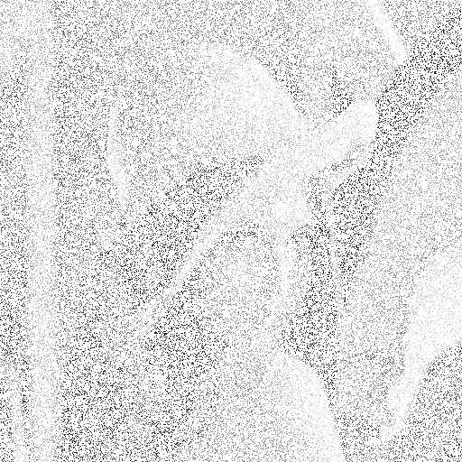
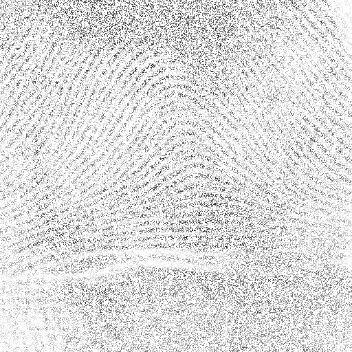
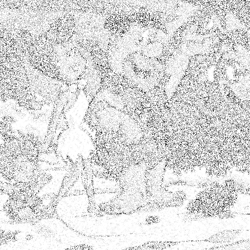
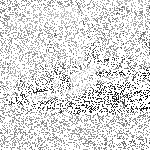
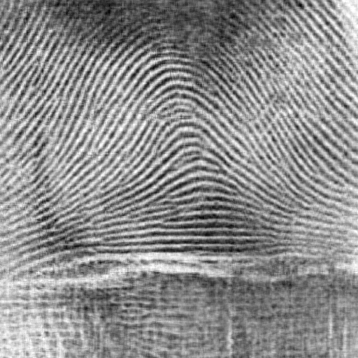
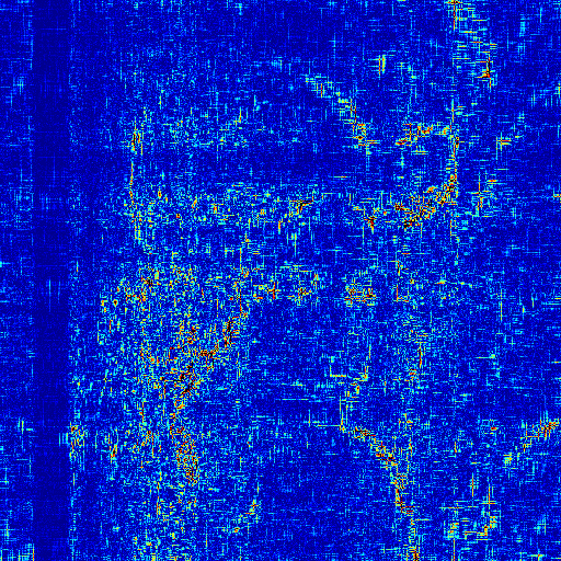
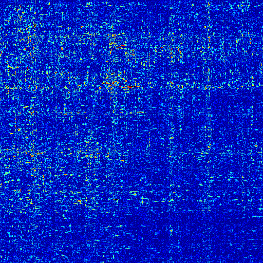
Figure 4: Image reconstruction using NNM and WSST. First line: observed pixels (white means non-observed). Second line: reconstruction using NNM. Third line: difference between truth and NNM (red is bad, blue is good). Fourth line: recovery using WSST. Fifth line: difference between truth and WSST.

3.2.4 Collaborative filtering

Now, we consider matrix completion for a real dataset: the MovieLens data. It contains 3 datasets, available on http://www.grouplens.org/:

• movie-100K: 100,000 ratings for 1682 movies by 943 users

• movie-1M: 1 million ratings for 3900 movies by 6040 users

• movie-10M: 10 million ratings and 100,000 tags for 10681 movies by 71567 users

The ranks of the users are integers between $1$ and $5$. In each 3 datasets, each user has rated at least $20$ movies. For our experiments, we simply choose uniformly at random half of the ratings of each user to form a subset $\Gamma$ of the entire subset $\Omega$ or ratings. Then, based on the ratings in $\Gamma$, we try to predict the ratings in $\Omega-\Gamma$. Since many entries are missing, we measure the accuracy of completion by computing the relative error in $\Omega-\Gamma$. If $\hat{A}$ is a reconstruction matrix, we reproduce in Table 1 below the values of

$$\mathrm{err}=\|{\mathcal{P}}_{\Omega-\Gamma}(\hat{A})-{\mathcal{P}}_{\Omega-\Gamma}(A_{0})\|_{2}/\|{\mathcal{P}}_{\Omega-\Gamma}(A_{0})\|_{2},$$ (3.14)

together with the rank used for the reconstruction. We observe in Table 1 that WSST improves a lot upon NNM on each datasets. The most surprising fact is that the rank used by WSST is much smaller than the one used by NNM, while leading at the same time to strong prediction improvements. For movie-1M for instance, the prediction error of WSST is $30\%$ better than NNM, while NNM solution has rank 200 and the WSST has rank 40. Once again, we can conclude on this example that WSST gives both much simpler reconstructions, and better prediction accuracy. Note that we considered a maximum rank equal to 200 for the movie-100K and movie-1M datasets, and equal to 50 for movie-10M (to make this problem computationally tractable on a normal computer).

			relative error		rank
	$n_{1}/n_{2}$	$m$
			NNM	WSST	NNM	WSST
movie-100K:	943/1682	1.00e+5	3.92e-01	3.30e-01	128	33
movie-1M:	6040/3702	1.00e+6	3.83e-01	2.70e-01	200	40
movie-10M:	71567/10674	9.91e+6	2.76e-01	2.36e-01	50	5

Table 1: Relative reconstruction errors for the MovieLens datasets.

4 Proofs

4.1 Proofs for Section 2

We denote by $\ell_{p}^{M}$ the space $\mathbb{R}^{M}$ endowed with the $\ell_{p}$ norm. The unit ball there is denoted by $B_{p}^{M}$. We also denote the unit Euclidean sphere in $\mathbb{R}^{M}$ by ${\cal S}^{M-1}$. We denote by $(e_{1},\ldots,e_{N})$ the canonical basis of $\mathbb{R}^{N}$ and for any $I\subset\{1,\ldots,N\}$ denote by $\mathbb{R}^{I}$ the subspace of $\mathbb{R}^{N}$ spanned by $(e_{i}:i\in I)$. Let $A=[A_{\{1\}},\ldots,A_{\{N\}}]$ be a matrix from $\mathbb{R}^{N}$ to $\mathbb{R}^{m}$, where $A_{\{i\}}$ denotes the $i$-th column vector of $A$. Let $x\in\mathbb{R}^{N}$ and $I$ an arbitrary subset of $\{1,\ldots,N\}$. We define $A_{I}=[A_{\{i\}}:i\in I]$ the matrix from $\mathbb{R}^{I}$ to $\mathbb{R}^{m}$ with columns vectors $A_{\{i\}}$ for $i\in I$. We denote by $x_{I}$ the vector in $\mathbb{R}^{I}$ with coordinates $x_{i}$ for $i\in I$, where $x_{i}$ is the $i$-th coordinate of $x$. We denote by $x^{I}$ the vector of $\mathbb{R}^{N}$ such that $x_{i}^{I}=0$ when $i\notin I$ and $x_{i}^{I}=x_{i}$ when $i\in I$. If $w\in\mathbb{R}^{N}$ has non negative coordinates, we denote by $wx$ the vector $(w_{1}x_{1},\ldots,w_{N}x_{N})$ and by $x/w$ the vector $(x_{1}/w_{1},\ldots,x_{N}/w_{N})$ with the previous convention in case where $w_{i}=0$ for some $i$. We denote by $|x|$ the vector $(|x_{1}|,\ldots,|x_{N}|)$. The support of $x$ is denoted by $I_{x}$, this is the set of all $i\in\{1,\ldots,N\}$ such that $x_{i}\neq 0$. We also consider the $w$-weighted $\ell_{1}^{N}$-norm

$$|x|_{1,w}=\sum_{i=1}^{N}\frac{|x_{i}|}{w_{i}}.$$ (4.1)

Note that $|\cdot|_{1,w}$ is a norm only when restricted to $\mathbb{R}^{I_{w}}$, where $I_{w}$ is the support of $w$.

We start with the well-known null space property and dual characterization [6] of exact reconstruction of a vector by $\ell_{1}$-based algorithms.

Proposition 1.

Let $x,w\in\mathbb{R}^{N}$ and denote by $I_{x}$ (resp. $I_{w}$) the support of $x$ (resp. $w$). The following points are equivalent:

1. $\Delta_{w}(Ax)=x$,

2. $I_{x}\subset I_{w}$ and for any $h\in\ker A_{I_{w}}$ such that $h\neq 0$ then

   $$\left|\Big{(}\frac{h}{w_{I_{w}}}\Big{)}_{I_{x}^{\complement}}\right|_{1}+\left\langle{\rm sgn}(x_{I_{x}}),\Big{(}\frac{h}{w_{I_{w}}}\Big{)}_{I_{x}}\right\rangle>0,$$

3. $I_{x}\subset I_{w}$ and there exists $Y\in(\ker A_{I_{w}})^{\bot}$ such that $(w_{I_{w}}Y)_{I_{x}}={\rm sign}(x_{I_{x}})$ and $|(w_{I_{w}}Y)_{I_{x}^{\complement}}|_{\infty}<1$.

Proof.

It follows from (2.3) that, under each one of the three conditions, we have $I_{x}\subset I_{w}$. Therefore, to simply notations, we can work as if the ambient space were $\mathbb{R}^{I_{w}}$. Hence, without loss of generality, we assume that $\mathbb{R}^{I_{w}}=\mathbb{R}^{N}$. We also denote by $I=I_{x}$ the support of $x$.

[Point 2. entails Point 1.] Using standard arguments (see for instance [44]), we can see that the subgradient of $|\cdot|_{1,w}$ at $x\in\mathbb{R}^{N}$ is the set

$$\begin{split}\partial|x|_{1,w}=\big{\{}t\in\mathbb{R}^{N}:t_{i}&={\rm sgn}(x_{i})/w_{i}\text{ when }x_{i}\neq 0\\ &\text{ and }|t_{i}|\leq 1/w_{i}\text{ when }x_{i}=0\big{\}}.\end{split}$$ (4.2)

Using the definition of the subgradient of $|\cdot|_{1,w}$ at $x$, it follows that for any $h\in\mathbb{R}^{N}$,

$$|x+h|_{1,w}\geq|x|_{1,w}+|(h/w)_{I^{\complement}}|_{1}+\bigl{<}{\rm sgn}(x_{I}),(h/w)_{I}\bigr{>}.$$

Thus, if Point 2 holds then for any $h\in\ker A$ such that $h\neq 0$,

$$|x+h|_{1,w}>|x|_{1,w}$$

and thus Point 1 is satisfied.

[Point 3. entails Point 2.] Let $Y\in(\ker A)^{\bot}$ such that $(wY)_{I}={\rm sgn}(x_{I})$ and $|(wY)_{I^{\complement}}|_{\infty}<1$. For any $h\neq 0$ in $\ker A$, we have

$$|(h/w)_{I^{\complement}}|_{1} +\bigl{<}{\rm sgn}(x_{I}),(h/w)_{I}\bigr{>}=\bigl{<}{\rm sgn}(x)^{I}+{\rm sgn}(h)^{I^{\complement}},h/w\bigr{>}$$

$$=\bigl{<}({\rm sgn}(x)/w)^{I}+({\rm sgn}(h)/w)^{I^{\complement}},h\bigr{>}$$

$$=\bigl{<}({\rm sgn}(x)/w)^{I}+({\rm sgn}(h)/w)^{I^{\complement}}-Y,h\bigr{>}$$

$$=\bigl{<}({\rm sgn}(h)/w)_{I^{\complement}}-Y_{I^{\complement}},h_{I^{\complement}}\bigr{>}=\sum_{i\in I^{\complement}}\frac{h_{i}}{w_{i}}\big{(}{\rm sgn}(h_{i})-w_{i}Y_{i}\big{)}>0,$$

where we used Point 3 in the fourth inequality.

[Point 1. entails Point 3.] This follows from classical results on the minimization of a convex function over a convex set (cf. [44]). Nevertheless, we provide a direct proof following the argument of [6]. Denote by $\{e_{1},\ldots,e_{N}\}$ the canonical basis in $\mathbb{R}^{N}$ and by $B_{1,w}^{N}$ the unit ball associated to the $w$-weighted $\ell_{1}^{N}$-norm:

$$B^{N}_{1,w}=\{t\in\mathbb{R}^{N}:|t|_{1,w}\leq 1\}.$$ (4.3)

If $x$ is the unique solution of (2.2) then $|x|_{1,w}B_{1,w}^{N}\cap(x+\ker A)=\{x\}$. Then by a duality argument (for instance Hahn-Banach Theorem for the separation of convex sets), there exists $Y\in\mathbb{R}^{N}$ such that $x+\ker A\subset\Gamma_{1}$, where $\Gamma_{1}=\{t:\bigl{<}t,Y\bigr{>}=1\}$ and $|x|_{1,w}B_{1,w}^{N}\subset\Gamma_{\leq 1}$, where $\Gamma_{\leq 1}=\{t:\bigl{<}t,Y\bigr{>}\leq 1\}$. Introduce $F_{1,w}(x)=|x|_{1,w}\mathop{\rm conv}(w_{i}e_{i}:x_{i}\neq 0)$, the face of $|x|_{1,w}B_{1,w}^{N}$ containing $x$. By moving the hyperplan $\Gamma_{1}$, we can assume that $|x|_{1,w}B_{1,w}^{N}\cap\Gamma_{1}\subset F_{1,w}(x)$. Since $|x|_{1,w}B_{1,w}^{N}\subset\Gamma_{\leq 1}$, we have $\sup_{t\in|x|_{1,w}B_{1,w}^{N}}\bigl{<}t,Y\bigr{>}\leq 1$ thus $|(wY)|_{\infty}\leq 1/|x|_{1,w}$. Moreover, $x\in\Gamma_{1}$ so $1=\bigl{<}x,Y\bigr{>}\leq|x|_{1,w}|(wY)|_{\infty}\leq 1$ because $|(wY)|_{\infty}\leq 1/|x|_{1,w}$. This is the equality case in Hölder’s inequality, so it follows that $(wY)_{I}={\rm sgn}(x_{I})/|x|_{1,w}$. Then, for any $i\notin I$, $|x|_{1,w}w_{i}e_{i}\in|x|_{1,w}B^{N}_{1,w}$, thus $\bigl{<}|x|_{1,w}w_{i}e_{i},Y\bigr{>}\leq 1$ and $|x|_{1,w}w_{i}e_{i}\notin F_{1,w}(x)$, so $|x|_{1,w}w_{i}e_{i}\notin\Gamma_{1}$ thus $\bigl{<}|x|_{1,w}w_{i}e_{i},Y\bigr{>}<1$. That is, $|(wY)_{I^{\complement}}|_{\infty}<1/|x|_{1,w}$. Finally, for any $h\in\ker A$, $1=\bigl{<}x+h,Y\bigr{>}=\bigl{<}x,Y\bigr{>}+\bigl{<}h,Y\bigr{>}=1+\bigl{<}h,Y\bigr{>}$, thus $\bigl{<}h,Y\bigr{>}=0$ and $Y\in(\ker A)^{\bot}$. Then, we normalize $Y$ by $|x|_{1,w}$ to obtain Point 3. ∎

Both Criterions 2 and 3 in Proposition 1 can be used to characterize the exact reconstruction of a vector $x$ by the $\ell_{1}$-weighted algorithm. The vector $Y$ of Criterion 3 is now called an exact dual certificate (cf. [6, 26]). We will use Criterion 3 and the construction of an exact dual certificate from [6] to prove Theorems 1 and 2. Note that Criterion 2 together with the construction of an inexact dual certificate (cf. [26]) can also be used. Nevertheless, we do not present this construction here since it does not improve the statement of Theorem 2.

4.1.1 Proof of Theorem 1

In the same way as we did in the proof of Proposition 1, we can work as if the ambient space were $\mathbb{R}^{I_{w}}$ and assume, without loss of generality, that $\mathbb{R}^{I_{w}}=\mathbb{R}^{N}$. We denote by $I$ the support of $x$. We prove first that when $\Delta_{1}(Ax)=x$, then $A_{I}$ is injective. Indeed, suppose that there exists some $h\in\mathbb{R}^{I}$ such that $h\neq 0$ and $A_{I}h=0$. Denote by $h^{0}\in\mathbb{R}^{N}$ the vector such that $h^{0}_{I}=h$ and $h^{0}_{I^{\complement}}=0$. We have $h^{0}\neq 0$ and $Ah^{0}=A_{I}h_{I}=0$. In particular, for any $\lambda\neq 0$, $\lambda h\in\ker A-\{0\}$. Therefore, since $x$ is the unique solution of the Basis Pursuit algorithm, it follows from Point 2 of Proposition 1 (applied to the weight vector $w=(1,\ldots,1)$), that, for every $\lambda\neq 0$, $\bigl{<}{\rm sgn}(x_{I}),\lambda h^{0}_{I}\bigr{>}>0.$ This is not possible, so $A_{I}$ is injective.

Since $\Delta_{1}(Ax)=x$, the decoder $\Delta_{2}$ is given here by

$$\Delta_{2}(Ax)\in\operatorname*{argmin}_{t\in\mathbb{R}^{N}}\Big{(}\sum_{i=1}^{N}\frac{|t_{i}|}{|x_{i}|}:At=Ax\Big{)}.$$

Therefore, according to (2.3), we have $\Delta_{2}(Ax)_{i}=0$ for any $i\notin I$, that is ${\rm supp}(\Delta_{2}(Ax))\subset I$. As a consequence $A_{I}x_{I}=Ax=A\Delta_{2}(Ax)=A_{I}\Delta_{2}(Ax)_{I}$ and $A_{I}$ is injective thus, $x_{I}=\Delta_{2}(Ax)_{I}$. Since $x_{I^{\complement}}=0=\Delta_{2}(Ax)_{I^{\complement}}$, we have $x=\Delta_{2}(Ax)$.

4.1.2 Proof of Theorem 2

We adapt to our setup the “dual certificate” introduced in [6] and consider

$$Y^{0}=A^{\top}A_{I}(A_{I}^{\top}A_{I})^{-1}\Big{(}\frac{{\rm sgn}(x)}{w}\Big{)}_{I}.$$ (4.4)

In particular, we have $Y^{0}\in\operatorname{im}(A^{\top})=(\ker A)^{\bot}$ and

$$Y_{I}^{0}=A^{\top}_{I}A_{I}(A_{I}^{\top}A_{I})^{-1}\Big{(}\frac{{\rm sgn}(x)}{w}\Big{)}_{I}=\Big{(}\frac{{\rm sgn}(x)}{w}\Big{)}_{I}.$$

Thus, we have $(wY^{0})_{I}={\rm sgn}(x_{I})$. In view of Proposition 1, it only remains to prove that $|(wY^{0})_{I^{\complement}}|<1$ with high probability. For $0<\delta<1$ and $\mu>0$, we consider the events

$$\Omega_{0}(I,\delta)=\big{\{}(1-\delta)|y|_{2}^{2}\leq|A_{I}y|_{2}^{2}\leq(1+\delta)|y|_{2}^{2},\quad\forall y\in\mathbb{R}^{I}\big{\}}$$ (4.5)

and

$$\Omega_{1}(I,\mu)=\big{\{}\max_{i\in I^{\complement}}|A_{I}^{\top}A_{\{i\}}|_{2}<\mu\big{\}}.$$ (4.6)

First, note that since $A_{I}^{\top}A_{I}-Id$ is Hermitian, we have

$$\|A_{I}^{\top}A_{I}-Id\|_{2\rightarrow 2}=\sup_{|y|_{2}=1}\big{|}|A_{I}y|_{2}^{2}-1\big{|}.$$

Thus, on $\Omega_{0}(I,\delta)$, we have $\|A_{I}^{\top}A_{I}-Id\|_{2\rightarrow 2}\leq\delta$ and so for any $y\in\mathbb{R}^{I}$, $\big{|}(A_{I}^{\top}A_{I})^{-1}y\big{|}_{2}\leq(1-\delta)^{-1}|y|_{2}$. In particular,

$$\Big{|}(A_{I}^{\top}A_{I})^{-1}\Big{(}\frac{{\rm sgn}(x)}{w}\Big{)}_{I}\Big{|}_{2}\leq\frac{1}{1-\delta}\Big{|}\Big{(}\frac{{\rm sgn}(x)}{w}\Big{)}_{I}\Big{|}_{2}=\frac{1}{1-\delta}\big{|}\big{(}1/w\big{)}_{I}\big{|}_{2}.$$

Then, it follows that, on $\Omega_{0}(I,\delta)\cap\Omega_{1}(I,x)$ and under condition $(A0)(I,(1-\delta)/\mu)$,

$$|(wY^{0})_{I^{\complement}}|_{\infty} =\max_{i\in I^{\complement}}\Big{|}w_{i}A_{\{i\}}^{\top}A_{I}(A_{I}^{\top}A_{I})^{-1}\Big{(}\frac{{\rm sgn}(x)}{w}\Big{)}_{I}\Big{|}$$

$$\leq\max_{i\in I^{\complement}}w_{i}\max_{i\in I^{\complement}}\Big{|}\bigl{<}A_{I}^{\top}A_{\{i\}},(A_{I}^{\top}A_{I})^{-1}\Big{(}\frac{{\rm sgn}(x)}{w}\Big{)}_{I}\bigr{>}\Big{|}$$

$$\leq\max_{i\in I^{\complement}}w_{i}\max_{i\in I^{\complement}}\big{|}A_{I}^{\top}A_{\{i\}}\big{|}_{2}\Big{|}(A_{I}^{\top}A_{I})^{-1}\Big{(}\frac{{\rm sgn}(x)}{w}\Big{)}_{I}\Big{|}_{2}$$

$$<\frac{\mu}{1-\delta}\max_{i\in I^{\complement}}w_{i}\big{|}\big{(}1/w\big{)}_{I}\big{|}_{2}\leq 1.$$

Then, Theorem 2 follows from the probability estimates of $\Omega_{0}(I,\delta)\cap\Omega_{1}(I,\mu)$ provided in the next lemma.

Lemma 4.1.

Let $A=m^{-1/2}\big{(}g_{i,j}\big{)}$ be a $m\times N$ matrix where the $g_{i,j}$’s are i.i.d. standard Gaussian variables. Assume that

$$m\geq c_{0}\max\Big{[}\frac{s}{\delta^{2}},\frac{s\log N}{\mu^{2}}\Big{]}.$$

With probability larger than $1-2\exp(-c_{1}m\delta^{2})-\exp(-c_{2}\mu^{2}m/s)$, we have

$$(1-\delta)|y|_{2}^{2}\leq|A_{I}y|_{2}^{2}\leq(1+\delta)|y|_{2}^{2},\quad\forall y\in\mathbb{R}^{I}$$

and $\max_{i\in I^{\complement}}|A_{I}^{\top}A_{\{i\}}|_{2}<\mu.$

Proof.

For the sake of completeness, we recall here the classical $\varepsilon$-net argument to prove the first statement of Lemma 4.1. It is enough to prove that $\sup_{y\in{\cal S}^{I}}||A_{I}y|_{2}^{2}-1|\leq\delta$, where ${\cal S}^{I}$ is the set of unit vectors of $\ell_{2}^{N}$ supported on $I$. First, note that

$$\sup_{y\in{\cal S}^{I}}\big{|}|A_{I}y|_{2}^{2}-1\big{|}=\sup_{y\in{\cal S}^{I}}|\bigl{<}Ty,y\bigr{>}|=\|T\|_{2\rightarrow 2},$$

where $T:\mathbb{R}^{I}\rightarrow\mathbb{R}^{I}$ is the symmetric operator $A^{\top}A-I_{d}$. Let $\Lambda\subset{\cal S}^{I}$ be a $1/4$-net of ${\cal S}^{I}$ for the $\ell_{2}$ metric with a cardinality smaller than $9^{s}$ (the existence of such a net follows from a volumetric argument, see [42]). For any $y\in{\cal S}^{I}$, there exists $z\in\Lambda$ such that $y=z+u$ with $\left|u\right|_{2}\leq 1/4$ and therefore,

$$|\bigl{<}Ty,y\bigr{>}|\leq|\bigl{<}Tz,z\bigr{>}|+|\bigl{<}Tu,u\bigr{>}|+2|\bigl{<}Tz,u\bigr{>}|\leq\max_{z\in\Lambda}|\bigl{<}Tz,z\bigr{>}|+\frac{9\|T\|_{2\rightarrow 2}}{16}.$$

Hence, $\|T\|_{2\rightarrow 2}\leq(16/7)\max_{z\in\Lambda}|\bigl{<}Tz,z\bigr{>}|$, and it is enough to control the supremum of $y\rightarrow|\bigl{<}Ty,y\bigr{>}|$ over $\Lambda$ instead of ${\cal S}^{I}$.

Let $y\in\Lambda$. We denote by $G_{1}/\sqrt{m},\ldots,G_{m}/\sqrt{m}$ the row vectors of $A$ where $G_{1},\ldots,G_{m}$ are $m$ independent standard Gaussian vectors of $\mathbb{R}^{N}$. We have $\bigl{<}Ty,y\bigr{>}=m^{-1}\sum_{i=1}^{m}\bigl{<}G_{i},y\bigr{>}^{2}-1$. Since $\|\bigl{<}G,y\bigr{>}^{2}\|_{\psi_{1}}=\|\bigl{<}G,y\bigr{>}\|_{\psi_{2}}^{2}$, it follows from Bernstein inequality for $\psi_{1}$ random variables [50] that

$$\mathbb{P}\big{[}|\bigl{<}Ty,y\bigr{>}|\leq\delta\big{]}\geq 1-2\exp(-c_{1}m\delta^{2}),$$

and a union bound yields

$$\mathbb{P}\big{[}|\bigl{<}Ty,y\bigr{>}|\leq\delta\;,\;\forall y\in\Lambda\big{]}\geq 1-2\exp(s\log 9-c_{1}m\delta^{2}).$$

Combining the $\varepsilon$-net argument with this probability estimate we obtain that when $m\geq c_{2}s/\delta^{2}$ then $\|T\|_{2\rightarrow 2}\leq\delta$ with probability at least $1-2\exp\big{(}-c_{3}m\delta^{2}\big{)}$.

Now, we turn to the second part of the statement. Let $i\in I^{\complement}$. The $i$-th column vector of $A$ is $A_{\{i\}}=G_{i}/\sqrt{m}=(g_{i1},\ldots,g_{im})^{\top}/\sqrt{m}$ where the $G_{i}$’s are independent standard Gaussian vectors of $\mathbb{R}^{m}$. Let $q\geq 2$ to be chosen later. By Markov inequality,

$$\mathbb{P}\Big{[}\Big{|}A_{I}^{\top}A_{\{i\}}\Big{|}_{2}\geq\mu\Big{]}=\mathbb{P}\Big{[}\Big{|}\sum_{j=1}^{m}g_{ij}G_{jI}\Big{|}_{2}\geq m\mu\big{]}\leq(m\mu)^{-q}\mathbb{E}\Big{|}\sum_{j=1}^{m}g_{ij}G_{jI}\Big{|}_{2}^{q}.$$ (4.7)

Now, we use the vectorial version of Khintchine inequality conditionally to $G_{1J},\ldots,G_{mJ}$, to obtain, for some absolute constant $c_{4}$,

$$\Big{(}\mathbb{E}_{g}\Big{|}\sum_{j=1}^{m}g_{ij}G_{jI}\Big{|}_{2}^{q}\Big{)}^{1/q}\leq c_{4}\sqrt{q}\Big{(}\mathbb{E}_{g}\Big{|}\sum_{j=1}^{m}g_{ij}G_{jI}\Big{|}_{2}^{2}\Big{)}^{1/2}=c_{4}\sqrt{q}\Big{(}\sum_{j=1}^{m}\big{|}G_{jI}\big{|}_{2}^{2}\Big{)}^{1/2}.$$

It follows that

$$\mathbb{E}\Big{|}\sum_{j=1}^{m}g_{ij}G_{jI}\Big{|}_{2}^{q}\leq\big{(}c_{4}^{2}qms\big{)}^{q/2}.$$

Hence, in (4.7) for $q=\big{(}\mu/(2c_{4}^{2})\big{)}^{2}(m/s)$, we obtain

$$\mathbb{P}\Big{[}\Big{|}A_{I}^{\top}A_{\{i\}}\Big{|}_{2}\geq\mu\Big{]}\leq\exp\Big{(}-\frac{\mu^{2}m\log 2}{s(2c_{4}^{2})^{2}}\Big{)}.$$

The result follows now from an union bound. ∎

4.1.3 Proof of Theorem 3

Proof.

Assume that $\Delta_{r}(Ax)=x$ and define $y=\Delta_{r+1}(Ax)$. By construction of $y$, we have $\operatorname{supp}(y)\subset\operatorname{supp}(x)$ and $Ax=Ay$. So, since $A$ is injective on $\Sigma_{m}$ and $x-y\in\Sigma_{m}$, we have $x=y$. This proves that $\Delta_{r+1}(Ax)=x$, and that the sequence $(\Delta_{n}(Ax))_{n}$ is constant and equal to a $\lfloor m/2\rfloor$-sparse vector starting from the $r$-th iteration.

Now, assume that there exists an integer $r$ and $y\in\Sigma_{\lfloor m/2\rfloor}$ such that $\Delta_{r}(Ax)=\Delta_{r+1}(Ax)=\cdots=y$. In particular, we have $Ay=Ax$, so since $A$ is injective on $\Sigma_{m}$ and $x-y\in\Sigma_{m}$, we have $x=y$. ∎

4.2 Proofs for Section 3

The next proposition shows that weighted spectral soft-thresholding achieves the minimum of the weighted nuclear norm plus a proximity term. Note that, however, weighted spectral soft-thresholding is not a proximal operator, since the weighted nuclear norm is not convex. This entails in particular that the proofs below use a direct analysis, since we cannot use arguments based on subdifferential computations here.

Proposition 2.

Let $B\in\mathbb{R}^{n_{1}\times n_{2}}$, $\tau,\lambda\geq 0$ and $w_{1}\geq\cdots\geq w_{n_{1}\wedge n_{2}}\geq 0$. Then the minimization problem

$$\min_{A\in\mathbb{R}^{n_{1}\times n_{2}}}\Big{\{}\frac{1}{2}\|A-B\|_{2}^{2}+\lambda\sum_{j=1}^{n_{1}\wedge n_{2}}\frac{\sigma_{j}(A)}{w_{j}}+\frac{\tau}{2}\|A\|_{2}^{2}\Big{\}}$$

has a unique solution, given by $\frac{1}{1+\tau}S_{\lambda}^{w}(B)$, where $S_{\lambda}^{w}(B)$ is the weighted soft-thresholding operator (3.12).

Proof of Proposition 2.

Denote for short $q=n_{1}\wedge n_{2}$ and write the SVD of $A$ as $A=U\Sigma V^{\top}=\sum_{j=1}^{q}\sigma_{j}u_{j}v_{j}^{\top}$ where $U=[u_{1},\ldots,u_{q}]$, $V=[v_{1},\ldots,v_{q}]$ and $\Sigma=\operatorname{diag}(\sigma_{1},\ldots,\sigma_{q})$. We have

$$\|A-B\|_{2}^{2}=\|B\|_{2}^{2}-2\sum_{j=1}^{q}\sigma_{j}u_{j}^{\top}Bv_{j}+(1+\tau)\sum_{j=1}^{q}\sigma_{j}^{2}$$

so that we want to minimize the function

$$\phi(U,V,\Sigma)=\frac{1}{2}\sum_{j=1}^{q}\Big{(}-2\sigma_{j}u_{j}^{\top}Bv_{j}+(1+\tau)\sigma_{j}^{2}\Big{)}+\lambda\sum_{j=1}^{q}\frac{\sigma_{j}}{w_{j}}$$

over $U,V,\Sigma$ with the constraints $U^{\top}U=I$, $V^{\top}V=I$ and $\sigma_{1}\geq\ldots\geq\sigma_{q}\geq 0$. Using the variational characterization of singular values, if $B=U^{\prime}\Sigma^{\prime}V^{\prime\top}$ is the SVD of $B$, where $U^{\prime}=[u_{1}^{\prime},\ldots,u_{q}^{\prime}]$, $V^{\prime}=[v_{1}^{\prime},\ldots,v_{q}^{\prime}]$, $\Sigma^{\prime}=\operatorname{diag}(\sigma_{1}^{\prime},\ldots,\sigma_{q}^{\prime})$, we know that the maximum of $u^{\top}Bv$ over all vectors $u$ and $v$ subject to $|u|_{2}=|v|_{2}=1$ and $u$ orthogonal to $u_{1}^{\prime},\ldots,u_{j-1}^{\prime}$ and $v$ orthogonal to $v_{1}^{\prime},\ldots,v_{j-1}^{\prime}$ is achieved at $u_{j}^{\prime}$ and $v_{j}^{\prime}$, and is equal to $\sigma_{j}^{\prime}$. So the maximum of $\phi(U,V,\Sigma)$ is achieved at $U=U^{\prime}$ and $V=V^{\prime}$, and

$$\phi(U^{\prime},V^{\prime},\Sigma)=\frac{1}{2}\sum_{j=1}^{q}\Big{(}-2\sigma_{j}\sigma_{j}^{\prime}+(1+\tau)\sigma_{j}^{2}+2\lambda\frac{\sigma_{j}}{w_{j}}\Big{)}.$$

It is easy to see that for each $j$ the the minimum over $\sigma_{j}$ is achieved at $\sigma_{j}=\frac{1}{1+\tau}(\sigma_{j}^{\prime}-\frac{\lambda}{w_{j}})_{+}$, which is non-increasing. ∎

As mentioned before, $S_{\lambda}^{w}$ is not a proximal operator. A nice property about proximal operators is that they are firmly non-expansive, see [44]. Namely, if $T$ is the proximal operator of some convex function over an Hilbert space $H$, then we have

$$\|Tx-Ty\|^{2}\leq\|x-y\|^{2}-\|x-y-(Tx-Ty)\|^{2}$$

for any $x,y\in H$. However, it turns out that we can prove, using a direct analysis, that $S_{\lambda}^{w}$ is non-expansive. Once again, the proof uses a direct and technical analysis (since we cannot use arguments based on subdifferential computations), while the property of firm-nonexpansivity of proximal operators is an easy consequence of their definition.

Proposition 3.

Let $w_{1}\geq\cdots\geq w_{n_{1}\wedge n_{2}}\geq 0,\lambda\geq 0$. Then, for any $A,B\in\mathbb{R}^{n_{1}\times n_{2}}$, we have

$$\|S_{\lambda}^{w}(A)-S_{\lambda}^{w}(B)\|_{2}\leq\|A-B\|_{2}.$$

Proof of Proposition 3.

Let us assume without loss of generality that $\lambda=1$. Write the SVD of $A$ and $B$ as $A=U_{1}\Sigma_{1}V_{1}^{\top}$ and $B=U_{2}\Sigma_{2}V_{2}^{\top}$ where $\Sigma_{1}=\operatorname{diag}[\sigma_{1,1},\ldots,\sigma_{1,r_{1}}]$, $\Sigma_{2}=\operatorname{diag}[\sigma_{2,1},\ldots,\sigma_{2,r_{2}}]$ and $r_{1}$ (resp. $r_{2}$) stands for the rank of $A$ (resp. $B$). We also write for short $\bar{A}=S_{1}^{w}(A)=U_{1}\bar{\Sigma}_{1}V_{1}^{\top}$ and $\bar{B}=S_{1}^{w}(B)=U_{2}\bar{\Sigma}_{2}V_{2}^{\top}$ where $\bar{\Sigma}_{1}=\operatorname{diag}[(\sigma_{1,1}-1/w_{1})_{+},\ldots,(\sigma_{1,r_{1}}-1/w_{r_{1}})_{+}]$ and $\bar{\Sigma}_{2}=\operatorname{diag}[(\sigma_{2,1}-1/w_{1})_{+},\ldots,(\sigma_{2,r_{1}}-1/w_{r_{2}})_{+}]$. We want to prove that $\|A-B\|_{2}^{2}-\|\bar{A}-\bar{B}\|_{2}^{2}\geq 0$. First use the decomposition

$$\|A-B\|_{2}^{2}- \|\bar{A}-\bar{B}\|_{2}^{2}=\|A\|_{2}^{2}-\|\bar{A}\|_{2}^{2}+\|B\|_{2}^{2}-\|\bar{B}\|_{2}^{2}-2\bigl{<}A,B\bigr{>}+2\bigl{<}\bar{A},\bar{B}\bigr{>}$$

$$=\sum_{j=1}^{r_{1}}\sigma_{1,j}^{2}-\sum_{j=1}^{\bar{r}_{1}}\Big{(}\sigma_{1,j}-\frac{1}{w_{j}}\Big{)}^{2}+\sum_{j=1}^{r_{2}}\sigma_{2,j}^{2}-\sum_{j=1}^{\bar{r}_{2}}\Big{(}\sigma_{2,j}^{2}-\frac{1}{w_{j}}\Big{)}^{2}$$

$$\quad-2\big{(}\bigl{<}A,B\bigr{>}-\bigl{<}\bar{A},\bar{B}\bigr{>}\big{)},$$

where we take $\bar{r}_{1}$ such that $\sigma_{1,j}>1/w_{j}$ for $j\leq\bar{r}_{1}$ and $\sigma_{1,j}\leq 1/w_{j}$ for $j\geq\bar{r}_{1}+1$, and similarly for $\bar{r}_{2}$. We decompose

$$\bigl{<}A,B\bigr{>}-\bigl{<}\bar{A},\bar{B}\bigr{>}=\bigl{<}A-\bar{A},B-\bar{B}\bigr{>}+\bigl{<}\bar{A},B-\bar{B}\bigr{>}+\bigl{<}A-\bar{A},\bar{B}\bigr{>}$$ (4.8)

Using von Neumann’s trace inequality $\bigl{<}X,Y\bigr{>}\leq\sum_{j}\sigma_{j}(X)\sigma_{j}(Y)$ (see for instance [28], Section 7.4.13), it follows for the first term of (4.8) that

$$\bigl{<}A-\bar{A},B-\bar{B}\bigr{>}\leq\sum_{j=1}^{r_{1}\wedge r_{2}}(\Sigma_{1}-\bar{\Sigma}_{1})_{j,j}(\Sigma_{2}-\bar{\Sigma}_{2})_{j,j}.$$

Using the same argument for the two other terms of (4.8), we obtain

$$\bigl{<}A,B\bigr{>}-\bigl{<}\bar{A},\bar{B}\bigr{>} \leq\sum_{j=1}^{r_{1}\wedge r_{2}}\Big{(}(\Sigma_{1}-\bar{\Sigma}_{1})_{j,j}(\Sigma_{2}-\bar{\Sigma}_{2})_{j,j}+(\bar{\Sigma}_{1})_{j,j}(\Sigma_{2}-\bar{\Sigma}_{2})_{j,j}$$

$$+(\Sigma_{1}-\bar{\Sigma}_{1})_{j,j}(\bar{\Sigma}_{2})_{j,j}\Big{)},$$

We explore the case $r_{1}\leq r_{2}$ and $\bar{r}_{1}\leq\bar{r}_{2}$; the other cases follow the same argument. We have

$$\bigl{<}A,B\bigr{>}-\bigl{<}\bar{A},\bar{B}\bigr{>}\leq\sum_{j=1}^{\bar{r}_{1}}\frac{\sigma_{1,j}}{w_{j}}+\Big{(}\sigma_{2,j}-\frac{1}{w_{j}}\Big{)}\frac{1}{w_{j}}+\sum_{j=\bar{r}_{1}+1}^{r_{1}}\sigma_{1,j}\sigma_{2,j},$$

so, an easy computation leads to

$$\|A-B\|_{2}^{2}-\|\bar{A}-\bar{B}\|_{2}^{2} \geq\sum_{j=\bar{r}_{2}+1}^{r_{1}}\sigma_{1,j}^{2}+\sum_{j=\bar{r}_{2}+1}^{r_{2}}\sigma_{2,j}^{2}-2\sum_{j=\bar{r}_{2}+1}^{r_{1}}\sigma_{1,j}\sigma_{2,j}$$

$$\quad+\sum_{j=\bar{r}_{1}+1}^{\bar{r}_{2}}\Big{(}\sigma_{1,j}^{2}-2\sigma_{1,j}\sigma_{2,j}+\frac{2\sigma_{2,j}}{w_{j}}-\frac{1}{w_{j}^{2}}\Big{)}.$$

We obviously have $\sum_{j=\bar{r}_{2}+1}^{r_{1}}\sigma_{1,j}^{2}+\sum_{j=\bar{r}_{2}+1}^{r_{2}}\sigma_{2,j}^{2}-2\sum_{j=\bar{r}_{2}+1}^{r_{1}}\sigma_{1,j}\sigma_{2,j}\geq 0$. By definition of $\bar{r}_{2}$ and $\bar{r}_{1}$, we have $\sigma_{1,j}\leq 1/w_{j}<\sigma_{2,j}$ for any $j=\bar{r}_{1}+1,\ldots,\bar{r}_{2}$. Hence, we have

$$\sigma_{1,j}^{2}-2\sigma_{1,j}\sigma_{2,j}+\frac{2\sigma_{2,j}}{w_{j}}-\frac{1}{w_{j}^{2}}=(\sigma_{1,j}-2\sigma_{2,j}+1/w_{j})(\sigma_{1,j}-1/w_{j})\geq 0,$$

which concludes the proof of Proposition 3. ∎

Proof of Theorem 4.

Consider the sequence $(A^{k})_{k\geq 0}$ defined in (3.13). Using Proposition 3 we have for any $k\geq 1$

$$\|A^{k+1}-A^{k}\|_{2} =\frac{1}{(1+\tau)}\|S_{\lambda}^{w}({\mathcal{P}}_{\Omega}(A_{0})+{\mathcal{P}}_{\Omega}^{\perp}(A^{k}))-S_{\lambda}^{w}({\mathcal{P}}_{\Omega}(A_{0})+{\mathcal{P}}_{\Omega}^{\perp}(A^{k-1}))\|_{2}$$

$$\leq\frac{1}{(1+\tau)}\|{\mathcal{P}}_{\Omega}^{\perp}(A^{k})-{\mathcal{P}}_{\Omega}^{\perp}(A^{k-1})\|_{2}\leq\frac{1}{(1+\tau)}\|A^{k}-A^{k-1}\|_{2},$$

so that $\|A^{k+1}-A^{k}\|_{2}\leq(1+\tau)^{-k}\|A^{1}-A^{0}\|_{2}.$ This proves that $\sum_{k\geq 0}\|A^{k+1}-A^{k}\|_{2}<+\infty$, so the limit of $(A^{k})_{k\geq 0}$ exists and is given by

$$A^{\infty}=\sum_{k\geq 0}(A^{k+1}-A^{k})+A^{0}.$$

Now, by continuity of $S_{\lambda}^{w}$ and ${\mathcal{P}}_{\Omega}^{\perp}$, taking the limit on both sides of (3.13), we obtain that $A^{\infty}$ satisfies the fixed-point equation

$$A^{\infty}=\frac{1}{1+\tau}S_{\lambda}^{w}({\mathcal{P}}_{\Omega}^{\perp}(A^{\infty})+{\mathcal{P}}_{\Omega}(A_{0})),$$

so we have found at least one solution. Let us show now that it is unique, so that $\hat{A}_{\lambda}^{w}=A^{\infty}$: consider a matrix $B$ satisfying the same fixed point equation. We have

$$\|B-A^{\infty}\|_{2} =\frac{1}{(1+\tau)^{2}}\|S_{\lambda}^{w}({\mathcal{P}}_{\Omega}(A_{0})+{\mathcal{P}}_{\Omega}^{\perp}(B))-S_{\lambda}^{w}({\mathcal{P}}_{\Omega}(A_{0})+{\mathcal{P}}_{\Omega}^{\perp}(A^{\infty}))\|_{2}$$

$$\leq\frac{1}{(1+\tau)}\|{\mathcal{P}}_{\Omega}^{\perp}(B)-{\mathcal{P}}_{\Omega}^{\perp}(A^{\infty})\|_{2}\leq\frac{1}{(1+\tau)}\|B-A^{\infty}\|_{2},$$

therefore $B=A^{\infty}$. ∎

Proof of Theorem 5.

We know from the proof of Theorem 4 that

$$\|\hat{A}_{\lambda}^{w}-A^{n}\|_{2}=\|\sum_{k\geq n}(A^{k+1}-A^{k})\|_{2}\leq\sum_{k\geq n}\frac{1}{(1+\tau)^{k}}\|A^{1}-A^{0}\|_{2},$$

leading to the conclusion. ∎

References

• [1] Jacob Abernethy, Francis Bach, Theodoros Evgeniou, and Jean-Phillipe Vert. Low-rank matrix factorization with attributes. Arxiv preprint cs/0611124, 2006.
• [2] Francis Bach, Rodolphe Jenatton, Mairal Julien, and Obozinski Guillaume. Convex optimization with sparsity-inducing norms, chapter 1. Optimization for Machine Learning,. MIT Press, 2011.
• [3] Amir Beck and Marc Teboulle. A fast iterative shrinkage-thresholding algorithm for linear inverse problems. SIAM J. Imaging Sci., 2(1):183–202, 2009.
• [4] Jian-Feng Cai, Emmanuel J. Candès, and Zuowei Shen. A singular value thresholding algorithm for matrix completion. SIAM J. Optim., 20(4):1956–1982, 2010.
• [5] Emmanuel J. Candès and Benjamin Recht. Exact matrix completion via convex optimization. Found. Comput. Math., 9(6):717–772, 2009.
• [6] Emmanuel J. Candès, Justin Romberg, and Terence Tao. Robust uncertainty principles: exact signal reconstruction from highly incomplete frequency information. IEEE Trans. Inform. Theory, 52(2):489–509, 2006.
• [7] Emmanuel J. Candès and Terence Tao. Decoding by linear programming. IEEE Trans. Inform. Theory, 51(12):4203–4215, 2005.
• [8] Emmanuel J. Candès and Terence Tao. Near-optimal signal recovery from random projections: universal encoding strategies? IEEE Trans. Inform. Theory, 52(12):5406–5425, 2006.
• [9] Emmanuel J. Candès and Terence Tao. Reflections on compressed sensing. IEEE Information Theory Society Newsletter, 58(4):14–17, 2008.
• [10] Emmanuel J. Candès and Terence Tao. The power of convex relaxation: near-optimal matrix completion. IEEE Trans. Inform. Theory, 56(5):2053–2080, 2010.
• [11] Emmanuel J. Candès, Michael B. Wakin, and Stephen P. Boyd. Enhancing sparsity by reweighted $l_{1}$ minimization. J. Fourier Anal. Appl., 14(5-6):877–905, 2008.
• [12] Antonin Chambolle and Pierre-Louis Lions. Image recovery via total variation minimization and related problems. Numer. Math., 76(2):167–188, 1997.
• [13] Rick Chartrand and Valentina Staneva. Restricted isometry properties and nonconvex compressive sensing. Inverse Problems, 24(3):035020, 14, 2008.
• [14] Rick Chartrand and Wotao Yin. Iteratively reweighted algorithms for compressive sensing. In Acoustics, Speech and Signal Processing, 2008. ICASSP 2008. IEEE International Conference on, pages 3869–3872. IEEE, 2008.
• [15] Scott Shaobing Chen, David L. Donoho, and Michael A. Saunders. Atomic decomposition by basis pursuit. SIAM J. Sci. Comput., 20(1):33–61, 1998.
• [16] Jon F. Claerbout and Francis Muir. Robust modeling of erratic data. Geophysics, 38:826–844, 1973.
• [17] Patrick L. Combettes and Valérie R. Wajs. Signal recovery by proximal forward-backward splitting. Multiscale Model. Simul., 4(4):1168–1200 (electronic), 2005.
• [18] Ingrid Daubechies, Ronald DeVore, Massimo Fornasier, and C. Sinan Güntürk. Iteratively reweighted least squares minimization for sparse recovery. Comm. Pure Appl. Math., 63(1):1–38, 2010.
• [19] Geoffrey Davis, Stephane Mallat, and Zhifeng Zhang. Adaptive time-frequency approximations with matching pursuits. In Wavelets: theory, algorithms, and applications (Taormina, 1993), volume 5 of Wavelet Anal. Appl., pages 271–293. Academic Press, San Diego, CA, 1994.
• [20] David L. Donoho. Compressed sensing. IEEE Trans. Inform. Theory, 52(4):1289–1306, 2006.
• [21] David L. Dononho. Reflections on compressed sensing. IEEE Information Theory Society Newsletter, 58(4):18–23, 2008.
• [22] Jordan Ellenberg. Fill in the blanks: Using math to turn lo-res datasets into hi-res samples. Wired, March 2010.
• [23] Maryam Fazel. Matrix rank minimization with applications. Elec Eng Dept Stanford University, 54:1–130, 2002.
• [24] Simon Foucart and Ming-Jun Lai. Sparsest solutions of underdetermined linear systems via $l_{q}$-minimization for $0<q\leq 1$. Appl. Comput. Harmon. Anal., 26(3):395–407, 2009.
• [25] Davis Goldberg, David Nichols, Brian M. Oki, and Douglas Terry. Using collaborative filtering to weave an information tapestry. Communications of the ACM, 35(12):61–70, 1992.
• [26] David Gross. Recovering low-rank matrices from few coefficients in any basis. Information Theory, IEEE Transactions on, 57(3):1548–1566, 2011.
• [27] David Gross, Yi Kai Liu, Steven T. Flammia, Stephen Becker, and Jens Eisert. Quantum state tomography via compressed sensing. Physical review letters, 105(15):150401, 2010.
• [28] Roger A. Horn and Charles R. Johnson. Matrix analysis. Cambridge University Press, Cambridge, 1985.
• [29] Shuiwang Ji and Jieping Ye. An accelerated gradient method for trace norm minimization. In Proceedings of the 26th Annual International Conference on Machine Learning, ICML ’09, pages 457–464, New York, NY, USA, 2009. ACM.
• [30] Raghunandan H. Keshavan, Andrea Montanari, and Sewoong Oh. Matrix completion from a few entries. IEEE Trans. Inform. Theory, 56(6):2980–2998, 2010.
• [31] Amin M. Khajehnejad, Weiyu Xu, Salman A. Avestimehr, and Babak Hassibi. Weighted $\ell_{1}$ Minimization for Sparse Recovery with Prior Information. ArXiv e-prints, January 2009.
• [32] Amin M. Khajehnejad, Weiyu Xu, Salman A. Avestimehr, and Babak Hassibi. Analyzing Weighted l1 Minimization for Sparse Recovery with Nonuniform Sparse Models. Signal Processing, IEEE Transactions on, pages 1–1, 2010.
• [33] Yong-Jin Liu, Defeng Sun, and Kim-Chuan Toh. An implementable proximal point algorithmic framework for nuclear norm minimization. Preprint, July, 2009.
• [34] Shiqian Ma, Donald Goldfarb, and Lifeng Chen. Fixed point and bregman iterative methods for matrix rank minimization. Mathematical Programming, pages 1–33, 2009. 10.1007/s10107-009-0306-5.
• [35] Stéphane G. Mallat and Zhifeng Zhang. Matching pursuits with time-frequency dictionaries. IEEE, Transactions on Signal Processing, 41(12):3397–3415, December 1993.
• [36] Rahul Mazumder, Trevor Hastie, and Robert Tibshirani. Spectral regularization algorithms for learning large incomplete matrices. Submitted to JMLR, 2009.
• [37] Mehran Mesbahi and G. P. Papavassilopoulos. On the rank minimization problem over a positive semidefinite linear matrix inequality. IEEE Trans. Automat. Control, 42(2):239–243, 1997.
• [38] Deanna Needell and Joel A. Tropp. CoSaMP: iterative signal recovery from incomplete and inaccurate samples. Appl. Comput. Harmon. Anal., 26(3):301–321, 2009.
• [39] Deanna Needell and Roman Vershynin. Uniform uncertainty principle and signal recovery via regularized orthogonal matching pursuit. Found. Comput. Math., 9(3):317–334, 2009.
• [40] Yurii E. Nesterov. A method for solving the convex programming problem with convergence rate $O(1/k^{2})$. Dokl. Akad. Nauk SSSR, 269(3):543–547, 1983.
• [41] Yurii E. Nesterov. Gradient methods for minimizing composite objective function. ReCALL, 76(2007076), 2007.
• [42] Gilles Pisier. The volume of convex bodies and Banach space geometry, volume 94 of Cambridge Tracts in Mathematics. Cambridge University Press, Cambridge, 1989.
• [43] Benjamin Recht. A simpler approach to matrix completion. CoRR, abs/0910.0651, 2009.
• [44] R. Tyrrell Rockafellar. Convex analysis. Princeton Mathematical Series, No. 28. Princeton University Press, Princeton, N.J., 1970.
• [45] Mark Rudelson and Roman Vershynin. On sparse reconstruction from Fourier and Gaussian measurements. Comm. Pure Appl. Math., 61(8):1025–1045, 2008.
• [46] Rayan Saab and Özgür Yılmaz. Sparse recovery by non-convex optimization—instance optimality. Appl. Comput. Harmon. Anal., 29(1):30–48, 2010.
• [47] Kim-Chuan Toh and Sangwoon Yun. An accelerated proximal gradient algorithm for nuclear norm regularized least squares problems. Pacific Journal of Optimization, 6(3):615–640, 2009.
• [48] Carlo Tomasi and Takeo Kanade. Shape and motion from image streams under orthography: a factorization method. International Journal of Computer Vision, 9(2):137–154, 1992.
• [49] Joel A. Tropp and Anna C. Gilbert. Signal recovery from random measurements via orthogonal matching pursuit. IEEE Trans. Inform. Theory, 53(12):4655–4666, 2007.
• [50] Aad W. van der Vaart and Jon A. Wellner. Weak convergence and empirical processes. Springer Series in Statistics. Springer-Verlag, New York, 1996. With applications to statistics.
• [51] Weiyu Xu, Amin M. Khajehnejad, Salman A. Avestimehr, and Babak Hassibi. Breaking through the Thresholds: an Analysis for Iterative Reweighted $\ell_{1}$ Minimization via the Grassmann Angle Framework. ArXiv e-prints, April 2009.