An MCMC Approach
to Universal Lossy Compression
of Analog Sources

Abstract

Motivated by the Markov chain Monte Carlo (MCMC) approach to the compression of discrete sources developed by Jalali and Weissman, we propose a lossy compression algorithm for analog sources that relies on a finite reproduction alphabet, which grows with the input length. The algorithm achieves, in an appropriate asymptotic sense, the optimum Shannon theoretic tradeoff between rate and distortion, universally for stationary ergodic continuous amplitude sources. We further propose an MCMC-based algorithm that resorts to a reduced reproduction alphabet when such reduction does not prevent achieving the Shannon limit. The latter algorithm is advantageous due to its reduced complexity and improved rates of convergence when employed on sources with a finite and small optimum reproduction alphabet.

I Introduction

Lossy compression of analog sources is a pillar of modern communication systems. Despite numerous applications such as image compression [2, 3], video compression [4], and speech coding [5, 6, 7], there is a significant gap between theory and practice.

I-A Entropy coding

Many practical lossy compression algorithms employ entropy coding, where scalar quantization is followed by lossless compression (ECSQ). ECSQ has motivated much work into optimization of scalar quantizers [8, 9, 10], whereas the translation to bits can use Huffman [11] or arithmetic [12, 13] codes. Despite the simplicity and elegance of ECSQ, even for independent and identically distributed (iid) sources the rate distortion (RD) function [14, 13], which characterizes the fundamental limit for lossy compression, suggests that ECSQ-based coding can be highly suboptimal (cf. Figure 1 for an example). For non-iid sources, ECSQ may compare even less favorably with the fundamental RD limit.

In order to bridge part of the gap between ECSQ and the RD function, vector quantization (VQ) converts an entire vector to a codeword [15, 7, 16], in contrast to scalar quantization, which compresses individual scalar input elements. VQ provides a better trade-off between rate and distortion as the vector dimension increases, but increased complexity is required [17]. The significant computation required by VQ necessitates developing computationally feasible alternatives.

I-B Related work

For finite alphabet sources, recent advances have demonstrated that the RD limit can be approached asymptotically [18, 19, 20] by partitioning an input into sub-blocks, where a Shannon-style codebook [13, 14] is applied to each sub-block. Some of these schemes can compress universally without knowing the source statistics beforehand, but it is challenging to generate a codebook distribution whose statistics differ from those of the input statistics [21].

Lossy compression over a finite alphabet can also be performed by directly mapping the entire input to an output sequence while accounting for the trade-off between the compressibility of the output and the distortion between the input and output sequences. This optimization can be deterministic [22] or stochastic [23] in nature. Directly mapping to the output sequence effectively quantizes the entire input – a long sequence – into a large output codebook, and achieves the RD limit for stationary ergodic finite alphabet sources universally. Another promising recent approach to (non-universal) lossy compression relies on algebraic codes [24].

For analog sources, less progress has been made in developing theoretically-justified compression algorithms. Some results have been derived specifically for the high-rate regime, where the Shannon lower bound is asymptotically tight [25]. In particular, in the limit of low distortions the RD limit has been characterized for mixtures of probability distribution functions (pdf’s) where one distribution is discrete and the other continuous [26, 27]. For example, the sparse Gaussian source is a mixture pdf; bounds on its RD function have been provided [28, 29, 30, 31].

Despite the theoretical insights in the high-rate regime, compression of analog sources at low-to-medium rates is of interest in many applications [2, 3, 4, 5]. There do exist special input pdf’s for which entropy coding approaches the RD function [32] in the low-rate limit, but the low-rate regime is challenging in general. We aspire to develop results of general applicability and not be limited to specific pdf’s with fortuitous properties.

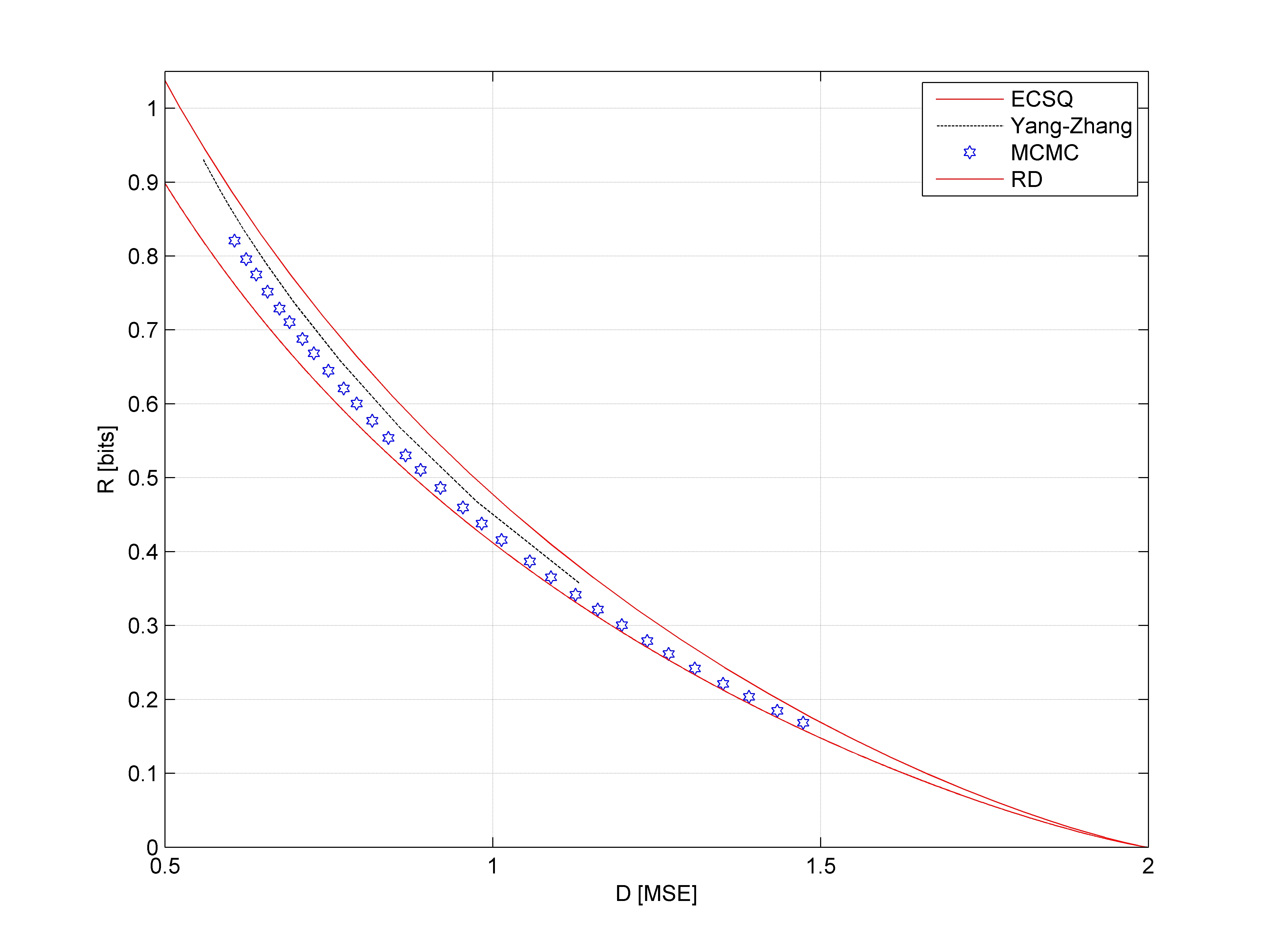
Figure 1: Laplace source: Comparison of entropy coding (ECSQ), results by Yang and Zhang [33], average rate and distortion of Algorithm 2 (MCMC) over 10 simulations, and the RD function. ($n=1.5\cdot 10^{4}$, $|{\cal{Z}}|=9$, $r=50$, $k\approx\frac{1}{2}\log_{|{\cal{Z}}|}(n)$.)

I-C Contributions

The crux of our approach to the compression of analog sources is to quantize to discrete reproduction levels, and then apply a compression algorithm similar to that of Jalali and Weissman [23], which uses the stochastic optimization approach of Markov chain Monte Carlo (MCMC) simulated annealing, as championed in [34]. A careful choice of the set of reproduction levels, growing appropriately with input length both in size and in resolution, achieves the RD function despite the analog nature of the source. A somewhat similar approach was suggested by Yang et al. [22, 33] using deterministic optimization techniques. Note, however, that Yang and Zhang [33] require availability of a training sequence, and so their algorithm is not universal. Although it is possible to apply deterministic optimization in a universal setting by partitioning the input into blocks, this approach results in a performance loss of 0.2–0.3 dB [33].

Our first contribution is a lossy compression algorithm for analog sources that relies on a data-independent reproduction alphabet that grows with the input length. This algorithm asymptotically achieves the RD function universally for stationary ergodic continuous amplitude sources. However, the reproduction alphabet grows with the input length, slowing down the convergence to the RD function, and is thus an impediment in practice.

To address this issue, we next propose an MCMC-based algorithm that uses an adaptive reproduction alphabet. The ground-breaking work by Rose on the discrete nature of the reproduction alphabet for iid sources when the Shannon lower bound is not tight [35] suggests that, for most sources of practical interest, restriction of the reconstruction to a rather small alphabet does not stand in the way of attaining the fundamental compression limits. Indeed, at low rates even a binary reproduction alphabet is often optimal [32]. When employed on such sources, our latter algorithm zeroes in on the finite reproduction alphabet, and thus enjoys rates of convergence commensurate with the finite-alphabet setting.

In order to render this adaptive algorithm computationally feasible, we develop a method to update the optimal reproduction levels rapidly. Utilizing this computational feature, our adaptive algorithm provides faster computation, achieves the RD function universally, and in some cases the smaller reproduction alphabet accelerates convergence to the RD function. Consequently, the adaptive algorithm is more suitable in practice. We emphasize that our algorithms are both universal, requiring no knowledge of the source statistics.

The remainder of the paper is organized as follows. We provide background information in Section II. Our first, brute force algorithm is described in Section III, followed by the adaptive reproduction alphabet algorithm in Section IV. Numerical results are reported in Section V. We complete the paper with a discussion in Section VI. Proofs appear in appendices, in order to make the main portion of the manuscript easily accessible.

II Background

II-A Notation

Consider a stationary ergodic source $X=\{X_{i},i\geq 1\}$ with real-valued components. We process a length-$n$ input ${x^{n}}=x_{1}x_{2}\ldots x_{n}$, which is an individual realization of the random vector $X^{n}$. The input ${x^{n}}$ is compressed using an encoder $e:{\cal{X}}$${}^{n}\rightarrow\{0,1\}$⁺ that maps ${x^{n}}$ to a finite output string $e({x^{n}})$. The decoder $d:\{0,1\}^{+}\rightarrow{\cal{Y}}$ⁿ maps the bit string back to a length-$n$ output ${y^{n}}$ over the reproduction alphabet ${\cal{Y}}$, which may be a continuous or discrete subset of the real line. The output ${y^{n}}$ is the lossy approximation of ${x^{n}}$.

We assess the performance of an encoder-decoder pair relative to the trade-off between rate and distortion [13, 14]. The rate of such a pair is defined as $R=E[\frac{1}{n}|e(X^{n})|]$, the expected number of bits per description of a source symbol, where $|\cdot|$ denotes length, size, or cardinality, and $E[\cdot]$ is expectation. The distortion $D=E[d_{n}(X^{n},{y^{n}})]$ quantifies the expected per-symbol distortion,

$$d_{n}({x^{n}},{y^{n}})\triangleq\frac{1}{n}\sum_{i=1}^{n}d(x_{i},y_{i}),$$ (1)

where $d:\mathbb{R}\times\mathbb{R}\rightarrow\mathbb{R}^{+}$ measures the distortion. For concreteness in what follows, we assume the distortion is the square of the error $d(x_{i},y_{i})=(x_{i}-y_{i})^{2}$, but our approach readily carries over to accommodate general distortion measures.

II-B Lossy compression using MCMC

We describe a variant of the scheme in [23] that compresses an input $x^{n}$ to an output $y^{n}$ over a finite alphabet ${\cal{Y}}\subseteq\mathbb{R}$. This algorithm will later be employed as the main building block for compressing an analog source. The encoder approximates ${x^{n}}$ by ${y^{n}}$, which is compressed using the context tree weighting (CTW) universal lossless compression algorithm. The approximation ${y^{n}}$ is chosen to provide a good trade-off between the coding length required for ${y^{n}}$ and the distortion with respect to ${x^{n}}$. The decoding procedure is straightforward; the output bits are passed through the CTW decompressor to retrieve ${y^{n}}$.

Denote the empirical symbol counts by $m_{k}({y^{n}},u^{k})[a]$, i.e.,

$$m_{k}({y^{n}},u^{k})[a]\triangleq|\{k<i\leq n:y_{i-k}^{i}=u^{k}a\}|,$$

where $k$ is the context depth, $a\in{\cal{Y}}$, $u^{k}\in{\cal{Y}}^{k}$, and $u^{k}a$ denotes concatenation of $u^{k}$ and $a$. Define the $k$-depth conditional empirical entropy as

$$H_{k}({y^{n}})\triangleq-\frac{1}{n}\sum_{a,u^{k}}m_{k}({y^{n}},u^{k})[a]\log\left(\frac{m_{k}({y^{n}},u^{k})[a]}{\sum_{a^{\prime}}m_{k}({y^{n}},u^{k})[a^{\prime}]}\right),$$ (2)

where $\log(\cdot)$ is the base-two logarithm, and we use the convention wherein $0\log(0)=0$. For $k=o(\log(n))$, the difference between the CTW coding length and the empirical conditional entropy is $o(1)$ [36]. We define the energy $\varepsilon({y^{n}})$ corresponding to ${y^{n}}$ by

$$\varepsilon({y^{n}})\triangleq n[H_{k}({y^{n}})-\beta d_{n}({x^{n}},{y^{n}})],$$ (3)

where $\beta<0$ is the slope of the RD function at the point we want to attain. The Boltzmann probability mass function (pmf) is

$$f_{s}({y^{n}})\triangleq\frac{1}{Z_{s}}\exp\{-s\varepsilon({y^{n}})\},$$ (4)

where $s>0$ is inversely related to temperature in simulated annealing [34], and $Z_{s}$ is the normalization constant.

Ideally, our goal is to compute the globally minimum energy solution ${\widehat{x^{n}}}$,

$${\widehat{x^{n}}}\triangleq\arg\min_{w^{n}\in{\cal{Y}}^{n}}\varepsilon(w^{n})=\arg\min_{w^{n}\in{\cal{Y}}^{n}}[H_{k}(w^{n})-\beta d_{n}({x^{n}},w^{n})].$$ (5)

Computation of ${\widehat{x^{n}}}$ involves an exhaustive search over exponentially many sequences and is thus infeasible. We use a stochastic Markov chain Monte Carlo (MCMC) relaxation [34] to approximate the globally minimum solution, in contrast to the deterministic approach of Yang et al. [22]. We denote the resulting approximation by ${y^{n}}$.

To sample from the Boltzmann pmf (4), we examine all $n$ locations. For each location, we use a Gibbs sampler to resample from the distribution of $y_{i}$ conditioned on $y^{n\backslash i}\triangleq\{y_{n}:\ n\neq i\}$ as induced by the joint pmf in (4), readily computed to be

$$f_{s}(y_{i}=a|y^{n\backslash i})=\frac{1}{\sum_{b}\exp\left\{-s\left[n\Delta H_{k}(y^{i-1}by_{i+1}^{n},a)-\beta\Delta d(b,a,x_{i})\right]\right\}},$$ (6)

where $\Delta H_{k}(y^{i-1}by_{i+1}^{n},a)$ is the change in $H_{k}({y^{n}})$ (2) when $y_{i}=a$ is replaced by $b$, and $\Delta d(b,a,x_{i})=d(b,x_{i})-d(a,x_{i})=(b-x_{i})^{2}-(a-x_{i})^{2}$ is the change in distortion. We refer to the resampling from a single location as an iteration, and group the $n$ possible locations into super-iterations.

During the simulated annealing, the inverse temperature $s$ is gradually increased, where in super-iteration $t$ we use $s=O(\log(t))$ [34, 23]. As the number of iterations $t$ is increased, ${y^{n}}$ converges in distribution to the set of minimal energy solutions, which includes ${\widehat{x^{n}}}$ (5), because large $s$ favors low-energy ${y^{n}}$. Pseudo-code for our encoder appears in Algorithm 1 below.

Algorithm 1: Lossy encoder with fixed reproduction alphabet Input: ${x^{n}}\in\mathbb{R}^{n}$, ${\cal{Y}}$, $\beta$, $c$, $r$ Output: bit-stream Procedure: 1. Initialize $y$ by quantizing $x$ with ${\cal{Y}}$ 2. Initialize $m_{k}(\cdot,\cdot)$ using $y$ 3. for $t=1$ to $r$ do // super-iteration 4. $s\leftarrow c\log(t)$ for some $c>0$ // inverse temperature 5. Draw permutation of numbers $\{1,\ldots,n\}$ at random 6. for $t^{\prime}=1$ to $n$ do 7. Let $i$ be component $t^{\prime}$ in permutation 8. Generate new $y_{i}$ using $f_{s}(y_{i}=\cdot|y^{n\backslash i})$ given in (6) // Gibbs sampling 9. Update $m_{k}(\cdot,\cdot)[\cdot]$ 10. Apply CTW to ${y^{n}}$ // compress outcome

III Universal algorithm with data-independent reproduction alphabet

Let us consider how Algorithm 1 can be used to compress analog sources. We will see that choosing the reproduction alphabet ${\cal{Y}}$ to be a finite subset of $\mathbb{R}$ (but growing with the input length $n$ in a data-independent way) achieves the RD function.

Let us assume that the variance of source symbols emitted by $X$ is finite, and consider the following data-independent reproduction alphabet,

$${\overline{{\cal{Y}}}}\triangleq\left\{-\frac{\gamma^{2}}{\gamma},-\frac{\gamma^{2}-1}{\gamma},\ldots,\frac{\gamma^{2}}{\gamma}\right\},\quad\gamma=\lceil\log(n)\rceil,$$ (7)

where $\lceil\cdot\rceil$ denotes rounding up. In words, ${\overline{{\cal{Y}}}}$ is a quantization of the interval $[-\gamma,\gamma]$ to resolution $1/\sqrt{\gamma}$. Other choices of ${\overline{{\cal{Y}}}}$ also allow to demonstrate various RD results; an examination of (22) indicates that slower-growing $\gamma(n)$ also achieves the RD function. The essential point is that ${\overline{{\cal{Y}}}}$ quantizes a wider interval with finer resolution as $n$ is increased, and its size increases sufficiently slowly with $n$.

To prove achievability of the RD function asymptotically, we first prove that a global optimization (5) that determines ${\widehat{x^{n}}}$ followed by lossless compression with CTW [36] achieves the RD function. Yang et al. [33, 22] proved a similar result for their deterministic algorithm while relying on a different reproduction alphabet; our contribution is to prove achievability using the data-independent reproduction alphabet ${\overline{{\cal{Y}}}}$.

Theorem 1

Consider square error distortion (1), let $X$ be a finite variance stationary and ergodic source with RD function $R(X,D)$, and use the data-independent reproduction alphabet ${\overline{{\cal{Y}}}}$ (7) to approximate ${x^{n}}$ by the globally minimum energy solution ${\widehat{x^{n}}}$ (5). Then the length of context tree weighting (CTW) [36] applied to ${\widehat{x^{n}}}$ converges as follows,

$$\lim_{n\rightarrow\infty}\sup E\left[\frac{1}{n}|CTW({\widehat{x^{n}}})|-\beta d_{n}({x^{n}},{\widehat{x^{n}}})\right]\leq\min_{D\geq 0}[R(X,D)-\beta D].$$ (8)

Note that the $\lim\sup$ in (8) is actually a limit since the expectation on the left hand side is lower bounded by the right hand side for any scheme and any $n$, cf., e.g., [22, 23]. The detailed proof appears in Appendix A, and we feature some highlights here. In order to prove achievability for the continuous alphabet source $X$, we construct a near-optimal codebook for a given input length $n$ [14], and then quantize the components of every codeword in the codebook to ${\overline{{\cal{Y}}}}$. As $n$ is increased, ${\overline{{\cal{Y}}}}$ quantizes a wider interval of values more finely. The wider interval ensures that outlier source symbols have a vanishing effect on the distortion, and finer quantization provides near-optimal distortion within the interval. Therefore, we have achievability for the continuous amplitude source $X$ via the finite alphabet ${\overline{{\cal{Y}}}}$.

Now consider running Algorithm 1 instead of the global energy minimization (5) using the data-independent reproduction alphabet ${\overline{{\cal{Y}}}}$. The constant $c$ used in Line 4 of Algorithm 1 plays a crucial role. If $c$ is large, then the Boltzmann pmf (4) favors low-energy sequences too greedily, and the algorithm might get stuck in local minima. On the other hand, there exists a universal constant $c_{1}$ such that for $c<c_{1}$ we obtain universal performance. To understand why this happens, observe that Algorithm 1 optimizes over $|{\overline{{\cal{Y}}}}|^{n}$ possible outputs. As long as $c<c_{1}$, there is a sufficiently large probability to transition between any two outputs, and the algorithm cannot get bogged down in a local mimimum. Therefore, in the limit of many iterations Algorithm 1 converges in distribution to the set of minimal energy solutions, and we enjoy the same RD performance as in Theorem 1. We refer the reader to Geman and Geman [34] for further discussions relating to the choice of $c_{1}$. The proof appears in Appendix B.

Theorem 2

Consider square error distortion (1), let $X$ be a finite variance stationary and ergodic source with RD function $R(X,D)$, and use Algorithm 1 with the data-independent reproduction alphabet ${\overline{{\cal{Y}}}}$ (7) and sufficiently small $c<c_{1}$. Let ${y^{n}_{r}}$ be the MCMC approximation to ${x^{n}}$ after $r$ super-iterations. Then the length of context tree weighting (CTW) [36] applied to ${y^{n}_{r}}$ converges as follows,

$$\lim_{n\rightarrow\infty}\lim_{r\rightarrow\infty}E\left[\frac{1}{n}|CTW({y^{n}_{r}})|-\beta d_{n}({x^{n}},{y^{n}_{r}})\right]\overset{n\rightarrow\infty}{\longrightarrow}\min_{D\geq 0}[R(X,D)-\beta D].$$

An important feature of the algorithm is that each iteration of Lines 7–9 requires computation that is proportional to the context depth $k$ and alphabet size $|{\overline{{\cal{Y}}}}|$, independent of $n$ [23]. Because the alphabet grows slowly in $n$, the per-iteration computational costs are modest. Each super-iteration contains $n$ iterations, and so its computation is $O(nk|{\overline{{\cal{Y}}}}|)=o(n\log^{3}(n))$. Decoding is also fast. We first decompress CTW [36], and the finite alphabet is then mapped to our data-independent reproduction alphabet ${\overline{{\cal{Y}}}}$.

It is also noteworthy that our results could be modified to support other distortion metrics. For example, if we used $\ell_{p}$ distortion, then a technical condition $E[|X|^{p}]<\infty$ ensures that outliers do not increase the distortion by much.

Although promising from a theoretical perspective, Algorithm 1 is of limited practical interest. In order to approach the RD function closely, ${\overline{{\cal{Y}}}}$ may need to be large, which slows down the algorithm. One approach to improve the algorithm is to encode outlier source symbols, i.e., $|x_{i}|>\gamma$, explicitly using $\approx\log(|x_{i}|/\gamma)$ bits, perhaps using a universal code for integers [38]. This encoder would reduce the distortion caused by outliers, thus allowing to use a narrower interval, yielding a reduction in the alphabet size. We leave the study of outlier processing for future work, and focus instead on using an adaptive reproduction alphabet to improve the algorithm.

IV Adaptive reproduction alphabet algorithm

Our approach to overcome the disadvantages of large alphabets (Section III) is inspired by the ground-breaking work by Rose on the discrete nature of the reproduction alphabet for iid sources when the Shannon lower bound is not tight [35]. In many cases of interest, a small reproduction alphabet achieves the RD function of an analog source. Indeed, at sufficiently low rates even a binary reproduction alphabet is sometimes optimal [32]. We thus focus on an algorithm that, while supporting the possibility that the reproduction alphabet must be large, also supports a possible reduction of the alphabet size, while allowing the actual reproduction levels to adapt to the input.

IV-A Adaptive reproduction levels

Following the approach of Yang and Zhang [33], we map the input ${x^{n}}$ to a sequence ${z^{n}}$ over a finite alphabet ${\cal{Z}}$, where the actual output ${y^{n}}$ is derived via a scalar function $y_{i}=a(z_{i})$. Ideally, the function $a(\cdot)$ should minimize expected distortion. Because we focus on square error distortion, the optimal $a^{*}(\cdot)$ is the conditional expectation [33],

$$a^{*}(\alpha)=E[x_{i}|z_{i}=\alpha],\ \forall\alpha\in{\cal{Z}}.$$ (9)

The decoder does not know ${x^{n}}$, and cannot compute $a^{*}(\cdot)$. Therefore, we encode the numerical value $a^{*}(\alpha)$ for each $\alpha\in{\cal{Z}}$. We allocate ${\mu}\log(\log(n))$ bits to encode each

$$a^{*}_{q}(\alpha)\triangleq\frac{\lceil a^{*}(\alpha)\Delta\rceil}{\Delta},$$ (10)

where $a^{*}_{q}(\alpha)$ is a quantized version of $a^{*}(\alpha)$, and the quantizer resolution $\frac{1}{\Delta}$ depends on ${\mu}$ and the width of the interval being quantized. We observe that it might be advantageous to allocate more bits to encode $a^{*}_{q}(\alpha)$ for symbols $\alpha\in{\cal{Z}}$ that appear more times in ${z^{n}}$, but leave such optimizations for future work. Nonetheless, if some $\alpha\in{\cal{Z}}$ does not appear in ${z^{n}}$, then there is no need to encode its numerical value. We expend one flag bit per character of ${\cal{Z}}$ to describe the effective alphabet ${{\cal{Z}}_{e}}={{\cal{Z}}_{e}}({z^{n}})$, where ${{\cal{Z}}_{e}}\subseteq{\cal{Z}}$ is the subset of the reproduction alphabet ${\cal{Z}}$ that appears in ${z^{n}}$. Because $|{\cal{Z}}|=|{\overline{{\cal{Y}}}}|=2\lceil\log(n)\rceil^{2}+1$, only $O(\log^{2}(n))$ flag bits are needed. In fact, it suffices for the encoder to describe the cardinality of ${{\cal{Z}}_{e}}$ using $O(\log(\log(n)))$ bits, which is insignificant.

The energy function (3) must be modified to support adaptive alphabets as follows,

$$\varepsilon_{a}({z^{n}})\triangleq n[H_{k}({z^{n}})-\beta d_{a}({x^{n}},{z^{n}})]+{\mu}\log(\log(n))|{{\cal{Z}}_{e}}({z^{n}})|,$$ (11)

where ${\mu}\log(\log(n))|{{\cal{Z}}_{e}}|$ bits are used to encode the reproduction levels that appear in the effective alphabet ${{\cal{Z}}_{e}}$, $d_{a}({x^{n}},{z^{n}})$ is distortion with the adaptive alphabet,

$$d_{a}({x^{n}},{z^{n}})=d_{n}({x^{n}},a^{*}_{q}({z^{n}}))=\frac{1}{n}\sum_{i=1}^{n}(x_{i}-a^{*}_{q}(z_{i}))^{2},$$ (12)

$a^{*}_{q}({z^{n}})$ is shorthand for the $n$-tuple obtained by applying $a^{*}_{q}$ to the components of ${z^{n}}$, and $a^{*}_{q}(\cdot)$ is computed using (9) and (10). These definitions require to modify the previous Gibbs sampler (6) as follows,

$$f_{s}(z_{i}=a|z^{n\backslash i})$$ (13)

$$= \frac{1}{\sum_{b}\exp\left\{-s\left[n\Delta H_{k}(z^{i-1}bz_{i+1}^{n},a)-\beta\Delta d_{a}(b,a,{z^{n}})+{\mu}\log(\log(n))\Delta{{\cal{Z}}_{e}}(b,a)\right]\right\}},$$

where

$$\Delta d_{a}(b,a,{z^{n}})\triangleq n\left[d_{a}({x^{n}},z^{i-1}bz_{i+1}^{n})-d_{a}({x^{n}},z^{i-1}az_{i+1}^{n})\right]$$ (14)

is the change in distortion using the adaptive alphabet (12), and $\Delta{{\cal{Z}}_{e}}(b,a)$ is the change in the size of the effective alphabet when $z_{i}=a$ is replaced by $b$. Alternately, the optimization routine can loop over different alphabet sizes $|{\cal{Z}}|$ without accounting for $|{\cal{Z}}|$ in the energy (11); this latter approach was used in our simulations (Section V).

The crux of the matter is that if a reduced alphabet yields similar distortion results without increasing the coding length, then the modified energy function (11) induces a smaller effective ${{\cal{Z}}_{e}}$. Motivated by the theoretical results by Rose [35] and our numerical results (Section V), for many analog sources of practical interest a small alphabet offers good and in many cases optimum RD performance. In such cases, the adaptive alphabet algorithm is advantageous.

Even if the entire alphabet is used, i.e., ${{\cal{Z}}_{e}}={\cal{Z}}$, then the location of the reproduction levels is optimized via $a^{*}(\cdot)$ in lieu of the uniform quantization used in ${\overline{{\cal{Y}}}}$ (7). Consequently, if we allow the adaptive alphabet algorithm to use ${\cal{Z}}$ with the same cardinality of ${\overline{{\cal{Y}}}}$ as in Algorithm 1, then the RD performance can only improve.

We now state formally that the adaptive alphabet algorithm achieves the RD function asymptotically without prior knowledge of the source statistics. As before, our result relies on the existence of a universal constant $c_{2}$ such that for $c<c_{2}$ the transition probabilities between the $|{\cal{Z}}|^{n}$ possible outputs are sufficiently large.

Theorem 3

Consider square error distortion (1), let $X$ be a finite variance stationary and ergodic source with RD function $R(X,D)$, use ${\cal{Z}}$ with cardinality $|{\cal{Z}}|=2\lceil\log(n)\rceil^{2}+1$ and sufficiently small $c<c_{2}$ in Algorithm 2, and let $a^{*}_{q}({z^{n}_{r}})$ be the MCMC approximation to ${x^{n}}$ after $r$ super-iterations. Then the length of context tree weighting (CTW) [36] applied to ${z^{n}_{r}}$ converges as follows,

$$\lim_{n\rightarrow\infty}\lim_{r\rightarrow\infty}E\left[\frac{1}{n}|CTW({z^{n}_{r}})|-\beta d_{a}({x^{n}},{z^{n}_{r}})\right]\overset{n\rightarrow\infty}{\longrightarrow}\min_{D\geq 0}[R(X,D)-\beta D].$$

The formal proof appears in Appendix C. The key point is that adaptive reproduction levels offer pointwise improvement over the data-independent reproduction alphabet ${\overline{{\cal{Y}}}}$ from Section III, per the same alphabet size.

IV-B Fast computation

An important contribution by Jalali and Weissman [23] was to show how to compute $\Delta H_{k}(y^{i-1}by_{i+1}^{n},a)$ and $\Delta d(b,a,x_{i})$ rapidly. Without this computational contribution, the encoder would be impractical. The adaptive algorithm updates $\Delta H_{k}(z^{i-1}bz_{i+1}^{n},a)$ in an analogous manner. However, whereas $\Delta d(b,a,x_{i})=(b-x_{i})^{2}-(a-x_{i})^{2}$ is trivial to compute for the data-independent reproduction alphabet ${\overline{{\cal{Y}}}}$ (7), in our case $\Delta d_{a}(b,a,{z^{n}})$ (14) requires to re-compute $d_{a}(\cdot,\cdot)$, which depends on $a^{*}_{q}(\cdot)$. Unfortunately, modifying a single location in ${z^{n}}$ may change the distortion for numerous symbols.

We now show how to compute $\Delta d_{a}(b,a,{z^{n}})$ rapidly for the adaptive reproduction alphabet algorithm. To do so, we evaluate $d_{a}({x^{n}},{z^{n}})$,

$$d_{a}({x^{n}},{z^{n}}) = \frac{1}{n}\sum_{i=1}^{n}d(x_{i},a^{*}_{q}(z_{i}))$$ (15)

$$= \frac{1}{n}\sum_{\alpha\in{\cal{Z}}}\sum_{\{i:\ z_{i}=\alpha\}}\left(x_{i}-a^{*}_{q}(\alpha)\right)^{2}$$ (16)

$$= \frac{1}{n}\sum_{\alpha\in{\cal{Z}}}\left\{\sum_{\{i:\ z_{i}=\alpha\}}\left[(x_{i})^{2}\right]-2a^{*}_{q}(\alpha)\left[x_{i}\right]+(a^{*}_{q}(\alpha))^{2}\left[1\right]\right\},$$ (17)

where (15) uses the definitions of $d_{n}(\cdot,\cdot)$ and $d_{a}(\cdot,\cdot)$ in (1) and (12), respectively, and (16) partitions $z_{i},\ i\in\{1,\ldots,n\}$, into the different symbols $\alpha\in{\cal{Z}}$ and invokes the definition of square error distortion. Combining (9) and (10),

$$a^{*}_{q}(\alpha)=\frac{\lceil E[x_{i}|z_{i}=\alpha]\Delta\rceil}{\Delta}=\frac{\left\lceil\frac{\sum_{\{i:\ z_{i}=\alpha\}}[x_{i}]}{\sum_{\{i:\ z_{i}=\alpha\}}[1]}\Delta\right\rceil}{\Delta}.$$ (18)

We see that (17) and (18) rely extensively on

$$X_{\alpha}^{m}\triangleq\sum_{\{i:\ z_{i}=\alpha\}}\left[(x_{i})^{m}\right],\quad m\in\{0,1,2\},\alpha\in{\cal{Z}},$$ (19)

the $m$’th moments of the portion of $x$ where $z_{i}=\alpha$. In each iteration of the algorithm, a single $z_{i}$ may change from $\alpha$ to $\alpha^{\prime}$. Consequently, we modify $X_{\alpha}^{m}$ and $X_{\alpha^{\prime}}^{m}$, $m\in\{0,1,2\}$, by adding and subtracting powers of $x_{i}$. Given these updated values, the computation of $\Delta d_{a}(b,a,{z^{n}})$ is rapid, as before. Pseudo-code for the adaptive alphabet Algorithm 2 appears below.

Algorithm 2: Lossy encoder with adaptive reproduction alphabet Input: ${x^{n}}\in\mathbb{R}^{n}$, ${\cal{Z}}$, $\beta$, $c$, $r$ Output: bit-stream Procedure: 1. Initialize $z$ by quantizing $x$ // can quantize with data-independent ${\overline{{\cal{Y}}}}$ 2. Initialize $m_{k}(\cdot,\cdot)$ and other data structures using $z$ 3. for $t=1$ to $r$ do super-iteration 4. $s\leftarrow c\log(t)$ for some $c>0$ // inverse temperature 5. Draw permutation of numbers $\{1,\ldots,n\}$ at random 6. for $t^{\prime}=1$ to $n$ do 7. Let $i$ be component $t^{\prime}$ in permutation 8. for all $\alpha$ in ${\cal{Z}}$ do // evaluate possible changes to $z_{i}$ 9. Compute $\Delta d_{a}(b,a,{z^{n}})$ via (14), (17), (18), and (19) 10. Compute $f_{s}(z_{i}=\alpha|z^{n\backslash i})$ given in (13) // modified Gibbs distribution 11. Generate new $z_{i}$ using $f_{s}(z_{i}=\cdot|z^{n\backslash i})$ // Gibbs sampling 12. Update $m_{k}(\cdot,\cdot)[\cdot]$ and $X_{z_{i}}^{m}$, $m\in\{0,1,2\}$ // previous and new $z_{i}$ 13. Encode effective alphabet ${{\cal{Z}}_{e}}$ 14. Encode $a^{*}_{q}(\alpha)$ using ${\mu}\log(\log(n))|{{\cal{Z}}_{e}}|$ bits 15. Apply CTW to ${z^{n}}$

As for the data-independent reproduction alphabet case, Algorithm 2 requires $O(nk|{\cal{Z}}|)$ time to compute $\Delta H_{k}(z^{i-1}bz_{i+1}^{n},a)$. Utilizing the computational techniques specified above, $\Delta d_{a}(b,a,{z^{n}})$ can be computed in constant time per inner loop of each iteration (Line 9), which requires $O(n|{\cal{Z}}|)=O(n|{\overline{{\cal{Y}}}}|)$ computation per super-iteration. We see that computing $\Delta H_{k}(z^{i-1}bz_{i+1}^{n},a)$ should require more time than computing $\Delta d_{a}(b,a,{z^{n}})$; this was confirmed in our implementation.

We have also noticed empirically that Algorithm 2 often comes quite close to optimum RD performance after a few dozen super-iterations, resulting in reasonable overall computational demands. Additionally, in practice the effective alphabet ${{\cal{Z}}_{e}}$ is often modest. CTW [36] converges to the empirical entropy as long as $k_{n}=\log(n)/\log(|{{\cal{Z}}_{e}}|)-\Omega_{n}(1)$, and for finite $n$ a smaller alphabet $|{{\cal{Z}}_{e}}|$ allows CTW to converge to the empirical entropy for larger context depths $k_{n}$. Therefore, Algorithm 2 can optimize over deeper context trees, leading to improved compression and faster convergence to the RD function.

The decoder of the adaptive reproduction alphabet Algorithm 2 resembles the decoder in [23]. First, the bit-stream generated by CTW is decompressed to reconstruct ${z^{n}}$. The actual real-valued reproduction sequence is obtained by mapping from ${z^{n}}$ to ${y^{n}}$ via the adaptive quantizer $a^{*}_{q}(\alpha)$, since the mapping $a^{*}_{q}$ has been described to the decoder.

V Numerical results

To demonstrate the potential of our approach, we implemented the adaptive alphabet Algorithm 2 in Matlab. Results for Laplace and autoregressive sources are provided.

Implementation details: We ran Algorithm 2 for sequences of length $n=1.5\cdot 10^{4}$ using $r=50$ super-iterations, and $k\approx\frac{1}{2}\log_{|{\cal{Z}}|}(n)$. We also found two heuristics to be useful. First, for each individual compression problem and RD slope $\beta$ the specific temperature evolution $s=O(\log(t))$ may vary. Therefore, for each point we ran four temperature evolution sequences and allowed each one to improve over the energy $\varepsilon_{a}({z^{n}})$ computed with previous evolution sequences. Second, using a good starting point helps Algorithm 2 converge. Therefore, we began running low rate problems with small $\beta$, and each solution was used as a starting point for the next larger $\beta$.

Below we plot results averaging over 10 simulations. Each plot compares the MCMC approach to entropy coding (ECSQ), results by Yang and Zhang [33], and the RD function.

Laplace source: We first evaluated an iid Laplace source with pdf $f(x)=\frac{1}{2}e^{-|x|}$ such that $E[X]=0$ and $\mbox{var}(X)=2$. For this source, entropy coding performs rather well. However, Yang and Zhang [33] give better RD performance (Figure 1). Algorithm 2 improves further over the deterministic minimization by Yang and Zhang [33], which requires availability of a training sequence. Their algorithm can be used in a universal setting by partitioning the input into blocks, resulting in a performance loss of 0.2–0.3 dB [33].

Relying on the mapping approach of Rose [35], it can be shown that for low-to-medium rates a small odd number of reproduction levels suffices to approach the fundamental RD limit. We have observed that the optimal mapping $a^{*}(\alpha)$ is similar to the reproduction alphabet computed by the mapping approach of Rose [35]. This similarity suggests that applying Algorithm 1 to the “correct” finite alphabet would not improve results by much.

Autoregressive source: Figure 2 illustrates the RD performance of the different algorithms for an autoregressive (AR) source, where

$$x_{n}=\rho x_{n-1}+w_{n},$$

$\rho=0.9$, and the innovation sequence $w_{n}\sim\cal{N}$$(0,1)$ is zero mean unit norm iid Gaussian.

Entropy coding (ECSQ) is not well suited for non-iid sources; vector quantization [17], the deterministic minimization algorithm by Yang and Zhang [33], and MCMC can be used instead. Note that ECSQ appears in the upper right hand side of the figure; its RD performance is poor.

We plotted the RD performance of Algorithm 2 using a small reproduction alphabet ($|{\cal{Z}}|=3$) and a moderately sized one ($|\mbox{${\cal{Z}}|$}=9$). At low rates, the smaller alphabet offers better RD performance; as the rate is increased, larger alphabets quantize the source more precisely. Although Algorithm 2 does not compress as well as Yang and Zhang (they describe the AR source as very challenging), recall that Algorithm 2 is universal.

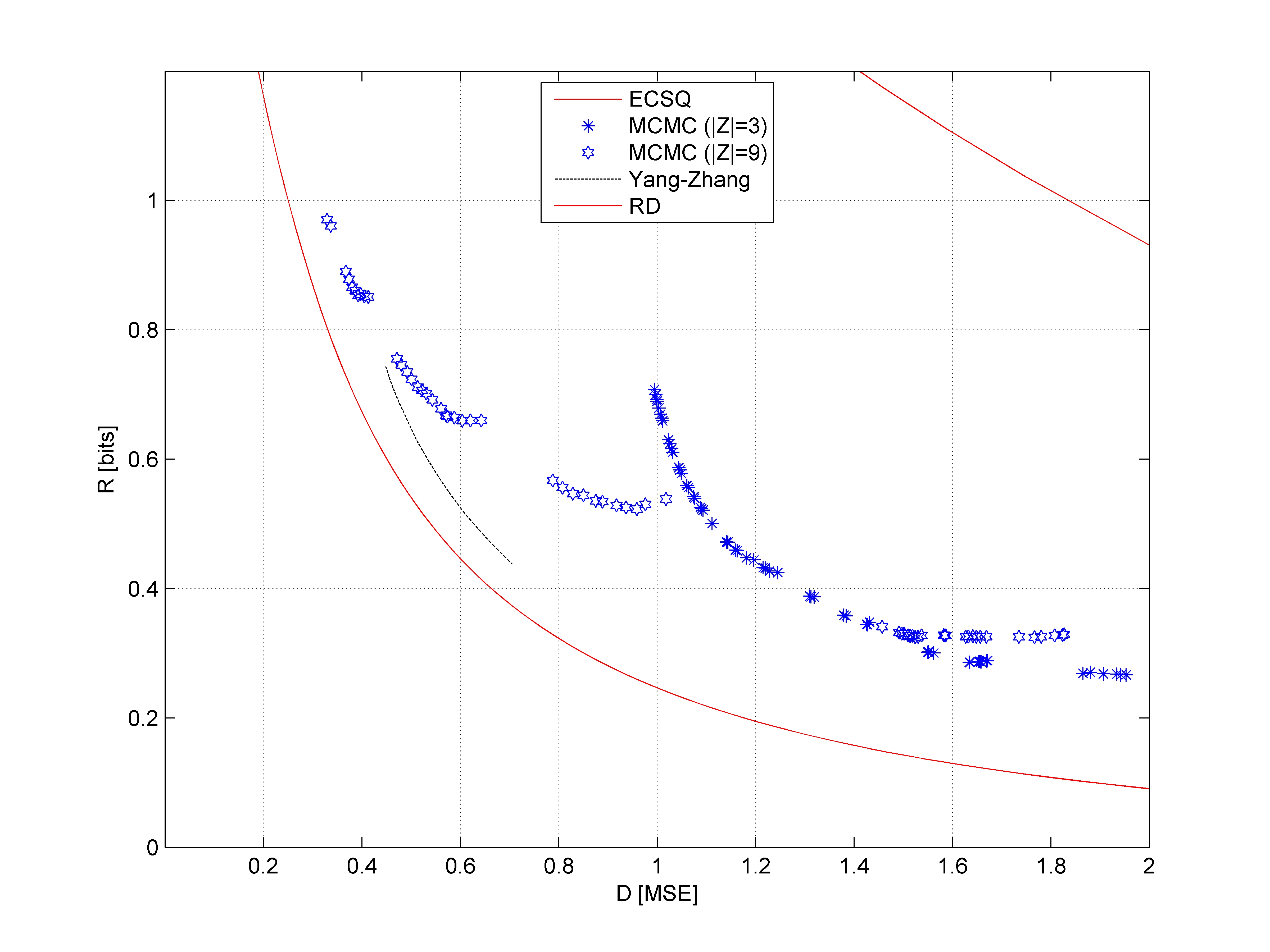
Figure 2: AR source: Comparison of entropy coding (ECSQ), average rate and distortion of Algorithm 2 (MCMC) over 10 simulations, results by Yang and Zhang [33], and the RD function. ($n=1.5\cdot 10^{4}$, $|{\cal{Z}}|$$\in\{3,9\}$, $r=50$, $k\approx\frac{1}{2}\log_{|{\cal{Z}}|}(n)$.)

VI Discussion

In this paper, we extended the MCMC simulated annealing approach of Jalali and Weissman [23] to analog sources. We described two lossy compression algorithms that asymptotically achieve the RD function universally for stationary ergodic continuous amplitude sources. The first algorithm relies on a data-independent reproduction alphabet that samples a wider interval with finer resolution as the input length is increased. However, the large alphabet slows down the convergence to the RD function, and is an impediment in practice. Our second algorithm therefore uses a (potentially smaller) adaptive reproduction alphabet. Not only is the adaptive algorithm theoretically motivated for iid sources by the discrete nature of the reproduction alphabet when the Shannon lower bound is not tight [35], but our numerical results suggest that even for non-iid sources it works well. Additionally, the smaller alphabet accelerates the computation.

Applications: In applications such as image compression [2, 3], video compression [4], and speech coding [5, 6, 7], our algorithms can process a vector of real-valued numbers whose statistics are either completely unknown, or perhaps only known approximately. The algorithms will then iterate over the data until some reasonable RD performance is attained.

As an example, consider image coding. The EQ coder [3] processes each sub-band of wavelets sequentially, going from low-frequency sub-bands and proceeding toward high-frequency sub-bands. The EQ coder classifies wavelet coefficients in each sub-band based on the magnitudes of parent coefficients, relying on the insight that the magnitudes of children coefficients are correlated with the magnitudes of parents [39]. In a similar manner, our algorithms can utilize the parent coefficients as contextual information.

Appendix A Proof of Theorem 1

Continuous codebook: We begin by constructing a continuous amplitude RD codebook [14]. Given the slope $\beta$ of the RD function $R(X,D)$, there exists an optimal rate $R(X,\beta)$ and distortion level $D(X,\beta)$. For any $\epsilon_{1}>0$, fix the rate $R=R(X,\beta)+\epsilon_{1}$. The achievable RD coding theorem [13, 14] demonstrates for the source $X$ that in the limit of large $n$ there exist codebooks whose rates are smaller than $R$ and whose expected per symbol distortions are less than $D(X,\beta)$. We choose such a codebook ${\cal{C}}$ comprised of at most $2^{Rn}$ codewords, each of length $n$. The encoder maps ${x^{n}}$ to the nearest codeword $c_{j}$ in ${\cal{C}}$ and transmits its index $j$. The decoder then maps index $j$ to $c_{j}$.

Quantized codebook: Now define a quantized codebook ${\overline{{\cal{C}}}}$ such that ${\overline{c_{ij}}}$, the $i$’th entry of the $j$’th codeword of ${\overline{{\cal{C}}}}$, is generated by rounding $c_{ij}$, the $i$’th entry of the $j$’th codeword of ${\cal{C}}$, to the closest value in ${\overline{{\cal{Y}}}}$. (Recall that $-\gamma$ and $\gamma$ are the smallest and largest values in ${\overline{{\cal{Y}}}}$, respectively.) Using ${\overline{{\cal{C}}}}$, the encoder and decoder are identical, except that ${\overline{c_{ij}}}$ is used instead of $c_{ij}$. The quantized codebook ${\overline{{\cal{C}}}}$ requires the same rate as before. However, the distortion provided by the quantized codebook ${\overline{{\cal{C}}}}$ is different.

Distortion of quantized codebook: To analyze the change in distortion, we consider three cases. In the first case, the original codebook value is an outlier whereas the signal value $x_{i}$ is not, i.e., $|c_{ij}|>\gamma$ and $|x_{i}|\leq\gamma$. The truncation of $|c_{ij}|$ to $\gamma$ reduces the distortion,

$$d(x_{i},{\overline{c_{ij}}})=(x_{i}-{\overline{c_{ij}}})^{2}<(x_{i}-c_{ij})^{2}=d(x_{i},c_{ij}).$$

The second case occurs when the original codebook and signal values are both outliers, i.e., $|x_{i}|,|c_{ij}|>\gamma$. As $n\rightarrow\infty$, the amount of variance beyond the increasing $\gamma=\lceil\log(n)\rceil$ vanishes, $E[(x_{i}\cdot 1_{\{|x_{i}|>\gamma(n)\}})^{2}]\overset{n\rightarrow\infty}{\longrightarrow}0$, because the source $X$ has finite variance and $\gamma$ increases (7). Therefore, for any $\delta_{1}>0$ there exists $N_{1}$ such that for all $n>N_{1}$ the increase in expected distortion $d_{n}({x^{n}},{y^{n}})$ (1) due to truncation of outliers is smaller than $\delta_{1}$. The third case occurs for $|c_{ij}|\leq\gamma$, where rounding changes the square error from $(x_{i}-c_{ij})^{2}$ to $(x_{i}-{\overline{c_{ij}}})^{2}$, and the distortion changes by

$$(x_{i}-{\overline{c_{ij}}})^{2}-(x_{i}-c_{ij})^{2} = ({\overline{c_{ij}}})^{2}-(c_{ij})^{2}+2x_{i}(c_{ij}-{\overline{c_{ij}}})$$

$$= (c_{ij}-{\overline{c_{ij}}})(2x_{i}-{\overline{c_{ij}}}-c_{ij})$$

$$= (c_{ij}-{\overline{c_{ij}}})\left[2(x_{i}-c_{ij})+(c_{ij}-{\overline{c_{ij}}})\right].$$

Because $|c_{ij}-{\overline{c_{ij}}}|\leq\frac{1}{2\gamma}$ (7), the change in distortion is upper bounded as follows,

$$|(x_{i}-{\overline{c_{ij}}})^{2}-(x_{i}-c_{ij})^{2}|\leq\frac{|x_{i}-c_{ij}|}{\gamma}+\frac{1}{4\gamma^{2}}.$$

We now define sets of indices that relate to the three cases,

$${\cal{I}}_{1} \triangleq \{i:\ i\in\{1,\ldots,n\},|c_{ij}|>\gamma,|x_{i}|\leq\gamma\},$$

$${\cal{I}}_{2} \triangleq \{i:\ i\in\{1,\ldots,n\},|x_{i}|,|c_{ij}|>\gamma\},$$

$${\cal{I}}_{3} \triangleq \{i:\ i\in\{1,\ldots,n\},|c_{ij}|\leq\gamma\}.$$

Summarizing over all $i\in\{1,\ldots,n\}$,

$$E\left[nd_{n}({x^{n}},{\overline{c_{j}}})\right] = E\left[\sum_{i=1}^{n}(x_{i}-{\overline{c_{ij}}})^{2}\right]$$ (20)

$$= E\left[\left[\sum_{i\in{\cal{I}}_{1}}(x_{i}-{\overline{c_{ij}}})^{2}\right]+\left[\sum_{i\in{\cal{I}}_{2}}(x_{i}-{\overline{c_{ij}}})^{2}\right]+\left[\sum_{i\in{\cal{I}}_{3}}(x_{i}-{\overline{c_{ij}}})^{2}\right]\right]$$

$$\leq E\left[\sum_{i\in{\cal{I}}_{1}}(x_{i}-c_{ij})^{2}\right]+E\left[\sum_{i\in{\cal{I}}_{2}}(x_{i}-c_{ij})^{2}+n\delta_{1}\right]$$

$$+E\left[\sum_{i\in{\cal{I}}_{3}}(x_{i}-c_{ij})^{2}+\frac{|x_{i}-c_{ij}|}{\gamma}+\frac{1}{4\gamma^{2}}\right]$$

$$\leq nE\left[d_{n}({x^{n}},c_{j})\right]+n\delta_{1}+\frac{E\left[\|{x^{n}}-c_{j}\|_{1}\right]}{\gamma}+\frac{n}{4\gamma^{2}},$$ (21)

where $c_{j}$ and ${\overline{c_{j}}}$ are the $j$’th codewords of ${\cal{C}}$ and ${\overline{{\cal{C}}}}$, respectively, $\|\cdot\|_{1}$ denotes the $\ell_{1}$ norm, the inequality in (20) relies on the changes in distortion in the three different cases, and the inequality in (21) is due to the $\gamma$ terms related to ${\cal{I}}_{3}$ that do not appear for ${\cal{I}}_{1}$ and ${\cal{I}}_{2}$. Because $E[d_{n}({x^{n}},c_{j})]\leq D$ and $\|{x^{n}}-c_{j}\|_{1}\leq n\sqrt{d_{n}({x^{n}},c_{j})}$, we have via Jensen’s inequality that $E[\|{x^{n}}-c_{j}\|_{1}]\leq n\sqrt{D}$. Therefore,

$$E[d_{n}({x^{n}},{\overline{c_{j}}})]<D+\delta_{1}+\frac{\sqrt{D}}{\gamma}+\frac{1}{4\gamma^{2}}=D+\delta_{1}+\frac{\sqrt{D}}{\lceil\log(n)\rceil}+\frac{1}{4\lceil\log(n)\rceil^{2}}.$$ (22)

Because $\gamma=\lceil\log(n)\rceil$ increases with $n$,

$$E[d({x^{n}},{\overline{c_{j}}})]\leq D+2\delta_{1}.$$ (23)

Therefore, the quantized codebook ${\overline{{\cal{C}}}}$ approaches the RD function asymptotically for the continuous amplitude source $X$.

Lossless compression using CTW: Having demonstrated that there exists a codebook based on the finite alphabet ${\overline{{\cal{C}}}}$ that asymptotically achieves the RD function, we need to prove that the RD performance of ${\overline{{\cal{C}}}}$ can be approached by compressing ${\widehat{x^{n}}}$ losslessly using CTW [36]. The remainder of the proof borrows from the prior art on lossy compression of finite sources [22, 23]. Owing to the linearity of expectation,

$$E\left[\frac{1}{n}|CTW({\widehat{x^{n}}})|-\beta d({x^{n}},{\widehat{x^{n}}})\right]=E\left[\frac{1}{n}|CTW({\widehat{x^{n}}})|-H_{k}({\widehat{x^{n}}})\right]+E\left[H_{k}({\widehat{x^{n}}})-\beta d({x^{n}},{\widehat{x^{n}}})\right].$$ (24)

Recall that $k=k_{n}=o(\log(n))$, and so for any $\epsilon_{2}>0$ there exists $N_{2}$ such that for all $n>N_{2}$ CTW converges to the empirical entropy [36],

$$E\left[\frac{1}{n}|CTW({\widehat{x^{n}}})|-H_{k}({\widehat{x^{n}}})\right]<\epsilon_{2},$$ (25)

as long as $k_{n}=\log(n)/\log(|{\overline{{\cal{Y}}}}|)-\Omega_{n}(1)$. Jalali and Weissman [23] invoke Gray et al. [40] to prove that for any $\delta_{2}>0$ and $\epsilon_{3}>0$ there exists a process $\widetilde{X}$ that is jointly stationary and ergodic with $X$ such that

$$E\left[H_{k}({\widehat{x^{n}}})-\beta d({x^{n}},{\widehat{x^{n}}})\right] \leq E\left[H_{k}(\widetilde{{x^{n}}})-\beta d({x^{n}},\widetilde{{x^{n}}})\right]$$ (26)

$$\leq H(\widetilde{X_{0}}|\widetilde{X_{-k}^{-1}})+\epsilon_{3}-E\left[\beta d({x^{n}},\widetilde{{x^{n}}})\right]$$ (27)

$$\leq R(X,D)+\epsilon_{4}+\epsilon_{3}-\beta(D(\beta)+\delta_{2}),$$ (28)

where (26) relies on the definition of ${\widehat{x^{n}}}$ (5), (27) is explained by observing that $H_{k}(\widetilde{{x^{n}}})$ converges to $H(\widetilde{X_{0}}|\widetilde{X_{-k}^{-1}})$ with probability one as $k_{n}$ is increased, and (28) uses properties of $\widetilde{X}$, i.e., $H(\widetilde{X_{0}}|\widetilde{X_{-k}^{-1}})\leq R(X,D)+\epsilon_{4}$ and $E\left[\beta d({x^{n}},\widetilde{{x^{n}}})\right]\leq D(\beta)+\delta_{2}$. Note also that $R(X,D)$ relies implicitly on $\beta$, and is identical to the $R(\beta)$ mentioned earlier. We complete the proof by combining (23), (24), (25), (28), and the arbitrariness of $\delta_{1}$, $\delta_{2}$, $\epsilon_{2}$, $\epsilon_{3}$, and $\epsilon_{4}$ $\Box$

Appendix B Proof of Theorem 2

The proof is similar to that by Jalali and Weissman [23, Appendix B], and we only outline the arguments here. While the algorithm is running, ${y^{n}_{r}}$ takes one of $|{\overline{{\cal{Y}}}}|^{n}$ possible values. These values are modeled as states of a Markov chain. There is a sufficiently positive probability to transition between any two states, because $c<c_{1}$ and each super-iteration of Algorithm 1 processes all $n$ locations of ${y^{n}}$. If the temperature is reduced slowly enough, then the distribution of ${y^{n}_{r}}$ converges toward the stationary distribution of the Markov chain. The proof is completed by noting that minimal-energy states occupy all the probabilistic mass of the stationary distribution. Therefore, ${y^{n}_{r}}$ converges in distribution to the set of minimal energy solutions, and we enjoy the same RD performance as in Theorem 1. $\Box$

Appendix C Proof of Theorem 3

The proof is similar to the proofs of Theorems 1 and 2. Consider the sequence ${\widehat{z^{n}}}$ with globally minimal modified energy (11),

$${\widehat{z^{n}}}\triangleq\arg\min_{w^{n}\in{\cal{Z}}^{n}}\varepsilon_{a}(w^{n}).$$ (29)

We first employ arguments from Appendix A to prove that ${\widehat{z^{n}}}$ achieves the RD function asymptotically. Next, we prove that simulated annealing [34] converges to the globally optimal solution asymptotically.

Achievable for global minimum: Recall that the adaptive algorithm uses ${\cal{Z}}$ with cardinality $|{\cal{Z}}|=|{\overline{{\cal{Y}}}}|$. Consider Appendix A, which proves that the globally optimal data-independent reproduction alphabet solution ${\widehat{x^{n}}}$ achieves the RD function asymptotically. Because $|{\cal{Z}}|=|{\overline{{\cal{Y}}}}|$, there exists a one to one mapping from ${\overline{{\cal{Y}}}}$ to ${\cal{Z}}$, and ${\widehat{x^{n}}}$ is mapped to some $\widetilde{{z^{n}}}$. The optimal $a^{*}(\cdot)$ may reduce the distortion,

$$d_{n}({x^{n}},a^{*}({\widehat{z^{n}}}))\leq d_{n}({x^{n}},{\widehat{x^{n}}}).$$

Although the quantized version $a^{*}_{q}(\cdot)$ may increase the distortion, i.e.,

$$d_{a}({x^{n}},{\widehat{z^{n}}})=d_{n}({x^{n}},a^{*}_{q}({\widehat{z^{n}}}))\geq d_{n}({x^{n}},a^{*}({\widehat{z^{n}}})),$$

allocating ${\mu}\log(\log(n))$ bits to encode each $a^{*}_{q}(\alpha)$ is sufficient to guarantee that the quantization error is smaller than $\frac{1}{\gamma}$ (see the proof of Theorem 1 in Appendix A). Our previous derivations (21), (22), (23) show that for any $\delta>0$ the overall distortion $d_{a}({x^{n}},{\widehat{z^{n}}})$ becomes $\delta$-close to $D(\gamma)$ as $n$ is increased. We conclude from the definitions of energy (3) and modified adaptive energy (11) that

$$\varepsilon_{a}({\widehat{z^{n}}})\leq\varepsilon({\widehat{x^{n}}})+n\beta\delta+{\mu}\log(\log(n))|{\overline{{\cal{Y}}}}|.$$

Because $|{\overline{{\cal{Y}}}}|=O(\log^{2}(n))$, the last term due to encoding the quantized $a^{*}_{q}(\cdot)$ vanishes relative to $n\beta\delta$. Taking $\delta$ as small as we want enables to approach $\min_{D\geq 0}[R(X,D)-\beta D]$ as closely as needed,

$$\lim_{n\rightarrow\infty}\sup E\left[\frac{1}{n}|CTW({\widehat{z^{n}}})|-\beta d_{a}({x^{n}},{\widehat{z^{n}}})\right]\leq\min_{D\geq 0}[R(X,D)-\beta D].$$

Invoking the converse result of Yang et al. [33, 22],

$$E\left[\frac{1}{n}|CTW({\widehat{z^{n}}})|-\beta d_{a}({x^{n}},{\widehat{z^{n}}})\right]\overset{n\rightarrow\infty}{\longrightarrow}\min_{D\geq 0}[R(X,D)-\beta D].$$

Simulated annealing: The proof is similar to that in Appendix B. The only noteworthy point is that for each ${z^{n}}$ the quantized $a^{*}_{q}(\cdot)$ is a deterministic function of ${z^{n}}$. Therefore, the simulated annealing can be posed as a Markov chain over $|{\cal{Z}}|^{n}$ states, where convergence in distribution to the set of minimal energy solutions is obtained by recognizing that for $c<c_{2}$ there is a sufficiently positive probability to transition between any two states. $\Box$

References

- [1] D. Baron and T. Weissman, “An MCMC approach to lossy compression of continuous sources,” in Proc. Data Compression Conf. (DCC), Mar. 2010, pp. 40–48.
- [2] Z. Xiong, K. Ramchandran, and M. T. Orchard, “Space-frequency quantization for wavelet image coding,” IEEE Trans. Image Process., vol. 6, no. 5, pp. 677–693, May 1997.
- [3] S. M. Lopresto, K. Ramchandran, and M. T. Orchard, “Image coding based on mixture modeling of wavelet coefficients and a fast estimation-quantization framework,” in Proc. Data Compression Conf. (DCC), Mar. 1997, pp. 221–230.
- [4] T. Wiegand, G. J. Sullivan, G. Bjontegaard, and A. Luthra, “Overview of the H.264/AVC video coding standard,” IEEE Trans. Circuits Syst. Video Technol., vol. 13, no. 7, pp. 560–576, Jul. 2003.
- [5] J. Makhoul, S. Roucos, and H. Gish, “Vector quantization in speech coding,” Proc. IEEE, vol. 73, no. 11, pp. 1551–1588, Nov. 1985.
- [6] A. Buzo, A. Gray Jr, R. Gray, and J. Markel, “Speech coding based upon vector quantization,” IEEE Trans. Acoustics, Speech and Signal Process., vol. 28, no. 5, pp. 562–574, 1980.
- [7] M. Sabin and R. Gray, “Product code vector quantizers for waveform and voice coding,” IEEE Trans. Acoustics, Speech and Signal Process., vol. 32, no. 3, pp. 474–488, 1984.
- [8] N. Farvardin and J. W. Modestino, “Optimum quantizer performance for a class of non-Gaussian memoryless sources,” IEEE Trans. Inf. Theory, vol. 30, no. 3, pp. 485–496, May 1984.
- [9] S. P. Lloyd, “Least squares quantization in PCM,” IEEE Trans. Inf. Theory, vol. 28, no. 2, pp. 129–137, Mar. 1982.
- [10] J. Max, “Quantization for minimum distortion,” IRE Trans. Inf. Theory, vol. 6, no. 1, pp. 7–12, Mar. 1960.
- [11] D. A. Huffman, “A method for the construction of minimum-redundancy codes,” Proc. Inst. Radio Eng., vol. 9, no. 40, pp. 1098–1101, Sep. 1952.
- [12] J. Rissanen and J. G. Langdon, “Universal modeling and coding,” IEEE Trans. Inf. Theory, vol. 27, no. 1, pp. 12–23, Jan. 1981.
- [13] T. M. Cover and J. A. Thomas, Elements of Information Theory. Wiley-Interscience, 1991.
- [14] T. Berger, Rate distortion theory; a mathematical basis for data compression. Prentice-Hall Englewood Cliffs, NJ, 1971.
- [15] P. Chou, T. Lookabaugh, and R. Gray, “Entropy-constrained vector quantization,” IEEE Trans. Acoustics, Speech and Signal Process., vol. 37, no. 1, pp. 31–42, 1989.
- [16] E. Riskin and R. Gray, “A greedy tree growing algorithm for the design of variable rate vector quantizers [image compression],” IEEE Trans. Signal Process., vol. 39, no. 11, pp. 2500–2507, 1991.
- [17] A. Gersho and R. M. Gray, Vector quantization and signal compression. Kluwer, 1993.
- [18] C. Gioran and I. Kontoyiannis, “Lossy compression in near-linear time via efficient random codebooks and databases,” CoRR, vol. abs/0904.3340, 2009.
- [19] A. Gupta, S. Verdú, and T. Weissman, “Linear-time near-optimal lossy compression,” in Proc. Int. Symp. Inf. Theory (ISIT2008), Jul. 2008.
- [20] I. Kontoyiannis, “An implementable lossy version of the Lempel-Ziv algorithm - Part I: Optimality for memoryless sources,” IEEE Trans. Inf. Theory, vol. 45, no. 7, pp. 2293–2305, Nov. 1999.
- [21] R. Zamir and K. Rose, “Natural type selection in adaptive lossy compression,” IEEE Trans. Inf. Theory, vol. 47, no. 1, pp. 99–111, Jan. 2001.
- [22] E. Yang, Z. Zhang, and T. Berger, “Fixed-slope universal lossy data compression,” IEEE Trans. Inf. Theory, vol. 43, no. 5, pp. 1465–1476, Sep. 1997.
- [23] S. Jalali and T. Weissman, “Rate-distortion via Markov chain Monte Carlo,” in Proc. Int. Symp. Inf. Theory (ISIT2008), Jul. 2008, pp. 852–856.
- [24] N. Hussami, S. B. Korada, and R. L. Urbanke, “Polar codes for channel and source coding,” CoRR, vol. abs/0901.2370, 2009.
- [25] T. Linder and R. Zamir, “On the asymptotic tightness of the Shannon lower bound,” IEEE Trans. Inf. Theory, vol. 40, no. 6, pp. 2026–2031, Nov. 1994.
- [26] A. György, T. Linder, and K. Zeger, “On the rate-distortion function of random vectors and stationary sources with mixed distributions,” IEEE Trans. Inf. Theory, vol. 45, no. 6, pp. 2110–2115, Sep. 1999.
- [27] H. Rosenthal and J. Binia, “On the epsilon entropy of mixed random variables,” IEEE Trans. Inf. Theory, vol. 34, no. 5, pp. 1110–1114, Sep. 1988.
- [28] C. Weidmann and M. Vetterli, “Rate distortion behavior of sparse sources,” 2008, submitted.
- [29] ——, “Rate-distortion analysis of spike processes,” in Proc. Data Compression Conf. (DCC), Mar. 1999, pp. 82–91.
- [30] R. Castro, M. B. Wakin, and M. Orchard, “On the problem of simultaneous encoding of magnitude and location,” in Asilomar Conf. Signals, Syst., Comput., 2002.
- [31] C. Chang, “On the rate distortion function of Bernoulli Gaussian sequences,” CoRR, vol. abs/0901.3820, 2009.
- [32] D. Marco and D. L. Neuhoff, “Low-resolution scalar quantization for Gaussian sources and squared error,” IEEE Trans. Inf. Theory, vol. 52, no. 4, pp. 1689–1697, Apr. 2006.
- [33] E. Yang and Z. Zhang, “Variable-rate trellis source encoding,” IEEE Trans. Inf. Theory, vol. 45, no. 2, pp. 586–608, Mar. 1999.
- [34] S. Geman and D. Geman, “Stochastic relaxation, Gibbs distributions, and the Bayesian restoration of images,” IEEE Trans. Pattern Anal. Mach. Intell., vol. 6, pp. 721–741, Nov. 1984.
- [35] K. Rose, “A mapping approach to rate-distortion computation and analysis,” IEEE Trans. Inf. Theory, vol. 40, no. 6, pp. 1939–1952, Nov. 1994.
- [36] F. M. J. Willems, Y. Shtarkov, and T. J. Tjalkens, “The context tree weighting method: Basic properties,” IEEE Trans. Inf. Theory, vol. 41, no. 3, pp. 653–664, May 1995.
- [37] J. Ziv and A. Lempel, “Compression of individual sequences via variable-rate coding,” IEEE Trans. Inf. Theory, vol. 24, no. 5, pp. 530–536, Sep. 1978.
- [38] P. Elias, “Universal codeword sets and representations of the integers,” IEEE Trans. Inf. Theory, vol. 21, no. 2, pp. 194–203, Mar. 1975.
- [39] S. Mallat, A wavelet tour of signal processing. Academic Press, 1999.
- [40] R. Gray, D. Neuhoff, and J. Omura, “Process definitions of distortion-rate functions and source coding theorems,” Trans. Inf. Theory, vol. 21, no. 5, pp. 524–532, Sep. 1975.