Quantum Master Equation and Filter for Systems Driven by Fields in a Single Photon State

Abstract

The aim of this paper is to determine quantum master and filter equations for systems coupled to continuous-mode single photon fields. The system and field are described using a quantum stochastic unitary model, where the continuous-mode single photon state for the field is determined by a wavepacket pulse shape. The master equation is derived from this model and is given in terms of a system of coupled equations. The output field carries information about the system from the scattered photon, and is continuously monitored. The quantum filter is determined with the aid of an embedding of the system into a larger system, and is given by a system of coupled stochastic differential equations. An example is provided to illustrate the main results.

I Introduction

In recent years single photon states of light have become increasingly important due to applications in quantum technology, in particular, quantum computing and quantum information systems, [20], [23], [18], [14], [26]. For instance, the light may interact with a system, say an atom, quantum dot, or cavity, and this system may be used as a quantum memory, [20], or to control the pulse shape of the single photon state [23]. Note that in practice one can consider different types of ‘single photon states’, including the single photon state of a single mode of light confined inside an optical cavity [20], or a single photon state superposed over a continuum of modes of a travelling field (i.e., colloquially, a “flying” single photon state) referred to as a continuous-mode or multimode single photon state [19], [22], [23]. In this paper we will be interested exclusively with the latter kind of single photon state and therefore from this point on when we say ‘single photon’ state we specifically mean the continuous-mode single photon state of a travelling field. When light interacts with a quantum system, information about the system is contained in the scattered light. This information may be useful for monitoring the behavior of the system, or for controlling it. The topic of this paper concerns the extraction of information from the scattered light when the incoming light is placed in a single photon state, denoted $|\xi\rangle$, as illustrated in Figure 1.

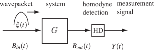
Figure 1: System $G$ coupled to a field in a continuous-mode single photon state $|\xi\rangle$ defined by the wavepacket $\xi$. The output field is continuously monitored by homodyne detection (assumed perfect) to produce a classical measurement signal $Y(t)$.

The problem of extracting information from continuous measurement of the scattered light is a problem of quantum filtering, [4], [5], [6], [10], [27], [3], [8], [28]. The current state of the art for quantum filtering considers incoming light in a vacuum or other Gaussian state, with quadrature or counting measurements. Single photon states of light are highly non-classical, and are fundamentally different from Gaussian states. At present, to the best of our knowledge, there are no filtering results for systems driven by single photon fields. In view of the increasing importance of single photon states of light, the purpose of this paper is to solve a quantum filtering problem for systems driven by single photon fields. As a by-product, we obtain a master equation for the system. A significant feature of the master equation and the quantum filter is that they are both given by a system of coupled equations, not a single equation as in the vacuum case. This reflects the non-Markovian character of systems driven by single photon fields.

The paper is organized as follows. The filtering problem to be solved is formulated in Section II. The master equation is derived in Section III using the model presented in Section II. This leads naturally to Section IV, where the system is embedded in a larger Markovian model, using a signal generator model. The single photon filter is presented in Section V, and an example is discussed in Section VI.

Notation: We use the standard Dirac notation $|\psi\rangle$ to denote state vectors (vectors in a Hilbert space) [21], [1]. The superscript ^∗ indicates Hilbert space adjoint or complex conjugate. The inner product of state vectors $|\psi_{1}\rangle$ and $|\psi_{2}\rangle$ is denoted $\langle\psi_{1}|\psi_{2}\rangle$. The expected value of an operator $X$ when the system is in state $|\psi\rangle$ is denoted $\mathbb{E}_{\psi}[X]=\langle\psi|X|\psi\rangle$. For operators $A$ and $B$ we write $\langle A,B\rangle=\mathrm{tr}[A^{\ast}B].$

II Problem Formulation

We consider a quantum system $G$ coupled to a quantum field $B_{in}$, as shown in Figure 1. The interaction of $B_{in}$ with $G$ produces the output field $B_{out}$. The input field is placed in a single photon state, denoted using Dirac’s notation as $|\xi\rangle$, where $\xi$ is a complex valued function such that $\int_{0}^{\infty}|\xi(s)|^{2}ds=1$. As illustrated in Figure 1, the wavepacket $|\xi\rangle$ interacts with the quantum system $G$, and the results of this interaction provide information about the system that may be obtained through continuous measurement of an observable $Y(t)$ of the output field $B_{out}(t)$. The filtering problem of interest in this paper is to determine the conditional state from which estimates $\hat{X}(t)$ of system operators $X$ may be determined at time $t$ based on knowledge of the observables $\{Y(s)$, $0\leq s\leq t\}$.

In what follows the system $G$ is assumed to be defined on a Hilbert space $\mathfrak{H}_{S}$, with an initial state denoted $|\eta\rangle\in\mathfrak{H}_{S}$. The input field $B_{in}$ is described in terms of annihilation $B(\xi)$ and creation $B^{\ast}(\xi)$ operators defined on a symmetric (Boson) Fock space $\mathfrak{F}$, [24, Chapter II], [8, Section 4]. The continuous-mode single photon state is defined on the symmetric Fock space by [19, sec. 6.3], [22, Section 14.2], [23, eq. (9)]

$$|\xi\rangle=B^{\ast}(\xi)|\phi\rangle,$$ (1)

where $|\phi\rangle$ is the vacuum state of the field. Expression (1) says that the single photon wavepacket is created from the vacuum using the field operator $B^{\ast}(\xi)$.

The Hilbert space for the composite system is

$$\mathfrak{H}=\mathfrak{H}_{S}\otimes\mathfrak{F}=\mathfrak{H}_{S}\otimes\mathfrak{F}_{t]}\otimes\mathfrak{F}_{(t},$$

where here we have exhibited the continuous temporal tensor product decomposition of the Fock space $\mathfrak{F}=\mathfrak{F}_{t]}\otimes\mathfrak{F}_{(t}$ into past and future components, which is of basic importance in what follows. We use the notation $\mathbb{E}$ to denote quantum expectation, usually with a subscript to denote the state being used. In particular, we write

$$\mathbb{E}_{11}[X\otimes F]=\langle\eta\xi|(X\otimes F)|\eta\xi\rangle=\langle\eta|X|\eta\rangle\langle\xi|F|\xi\rangle$$ (2)

for the expectation with respect to the product state $|\eta\xi\rangle$, where the field is in the single photon state. Here and in what follows $X$ is a bounded system operator acting on $\mathfrak{H}_{S}$, and $F$ is a field operator acting on the Fock space $\mathfrak{F}$. Similarly, we may define the expectation when the field is in the vacuum state,

$$\mathbb{E}_{00}[X\otimes F]=\langle\eta\phi|(X\otimes F)|\eta\phi\rangle=\langle\eta|X|\eta\rangle\langle\phi|F|\phi\rangle.$$ (3)

We will also have need for the cross-expectations

$$\mathbb{E}_{10}[X\otimes F]=\langle\eta\xi|(X\otimes F)|\eta\phi\rangle,$$

$$\mathbb{E}_{01}[X\otimes F]=\langle\eta\phi|(X\otimes F)|\eta\xi\rangle.$$ (4)

A crucial difference between the single photon state and the vacuum state is that the later state factorizes $|\phi\rangle=|\phi_{t]}\rangle\otimes|\phi_{(t}\rangle$ with respect to the temporal factorization $\mathfrak{F}=\mathfrak{F}_{t]}\otimes\mathfrak{F}_{(t}$ of the Fock space, with $|\phi_{t]}\rangle\in\mathfrak{F}_{t]}$ and $|\phi_{(t}\rangle\in\mathfrak{F}_{(t}$, while the former does not. Rather, we have

$$|\xi\rangle=B^{\ast}(\xi)|\phi\rangle=|\xi_{t]}\rangle\otimes|\phi_{(t}\rangle+|\phi_{t]}\rangle\otimes|\xi_{(t}\rangle,$$ (5)

where

$$|\xi_{t]}\rangle=B^{-\ast}_{t}(\xi)|\phi_{t]}\rangle,\ \text{and}\ |\xi_{(t}\rangle=B^{+\ast}_{t}(\xi)|\phi_{(t}\rangle,$$ (6)

and $B^{-}_{t}(\xi)=B(\xi\chi_{[0,t]})$, $B^{+}_{t}(\xi)=B(\xi\chi_{(t,\infty)})$, $B(\xi)=B^{-}_{t}(\xi)+B^{+}_{t}(\xi)$. Here, $\chi_{[0,t]}$ is the indicator function for the time interval $[0,t]$. Note that while $|\xi\rangle$ has unit norm, we have

$$\parallel|\xi_{t]}\rangle\parallel^{2}=\int_{0}^{t}|\xi(s)|^{2}ds,\ \text{and}\ \parallel|\xi_{(t}\rangle\parallel^{2}=\int_{t}^{\infty}|\xi(s)|^{2}ds.$$ (7)

A consequence of the additive decomposition (5) is the following. Let $K(t)$ be a bounded operator acting on the full Hilbert space $\mathfrak{H}$ that is adapted, i.e. $K(t)$ acts trivially on $\mathfrak{F}_{(t}$, the field in the future. Then the expectation with respect to the single photon field may be expressed in terms of the vacuum state as follows:

$$\mathbb{E}_{11}[K(t)] = \mathbb{E}_{00}[B^{-}_{t}(\xi)K(t)B^{-\ast}_{t}(\xi)+w(t)K(t)]$$ (8)

where $w(t)=\int_{t}^{\infty}|\xi(s)|^{2}ds$.

The dynamics of the system will be described using the quantum stochastic calculus, [17], [11], [24], [12], [8]. Quantum stochastic integrals are defined in terms of fundamental field operators $B(t)$, $B^{\ast}(t)$ and $\Lambda(t)$, [24, Chapter II], [8, Section 4]. The non-zero Ito products for the field operators are

$$dB(t)dB^{\ast}(t)=dt,\ \ dB(t)d\Lambda(t)=dB(t),\$$

$$d\Lambda(t)d\Lambda(t)=d\Lambda(t),\ \ d\Lambda(t)dB^{\ast}(t)=dB^{\ast}(t).$$ (9)

The dynamics of the composite system is described by a unitary $U(t)$ solving the Schrödinger equation, or quantum stochastic differential equation (QSDE),

$$dU(t)=\{(S-I)d\Lambda(t)+LdB^{\ast}(t)-L^{\ast}SdB(t)$$

$$-(\frac{1}{2}L^{\ast}L+iH)dt\}U(t),$$ (10)

with initial condition $U(0)=I$. Here, $H$ is a fixed self-adjoint operator representing the free Hamiltonian of the system, and $L$ and $S$ are system operators determining the coupling of the system to the field, with $S$ unitary. In this paper, for simplicity we assume that the parameters $G=(S,L,H)$ are bounded operators on the system Hilbert space $\mathfrak{H}_{S}$.

A system operator $X$ at time $t$ is given in the Heisenberg picture by $X(t)=j_{t}(X)=U(t)^{\ast}(X\otimes I)U(t)$ and it follows from the quantum Ito calculus that

$$dj_{t}(X) = j_{t}(S^{\ast}XS-X)d\Lambda(t)+j_{t}(S^{\ast}[X,L])dB(t)^{\ast}$$ (11)

$$+j_{t}([L^{\ast},X]S)dB(t)+j_{t}(\mathcal{G}(X))dt,$$

where

$$\mathcal{G}(X)=\mathcal{L}_{L}(X)-i[X,H],$$ (12)

and

$$\mathcal{L}_{L}(X)=\frac{1}{2}L^{\ast}[X,L]+\frac{1}{2}[L^{\ast},X]L.$$ (13)

and The map $X\mapsto\mathcal{G}(X)$ is known as the Lindblad generator, while the quartet of maps $X\mapsto\mathcal{G}(X),S^{\ast}XS-X,\,S^{\ast}[X,L],\,[L^{\ast},X]S$ are known as Evans-Hudson maps.

The output field is defined by $B_{out}(t)=U^{\ast}(t)B(t)U(t)$. In this paper we consider the output field observable $Y(t)$ defined by

$$Y(t)=U^{\ast}(t)Z(t)U(t),$$ (14)

where

$$Z(t)=B(t)+B^{\ast}(t),$$ (15)

is a quadrature observable of the input field. Note that both $Z(t)$ and $Y(t)$ are self-adjoint and self-commutative: $[Z(t),Z(s)]=0$ and $[Y(t),Y(s)]=0$. We write $\mathscr{Z}_{t}$ and $\mathscr{Y}_{t}$ for the subspaces of commuting operators generated by the observables $Z(s)$, $Y(s)$, $0\leq s\leq t$, respectively. They are related by the unitary rotation $\mathscr{Y}_{t}=U^{\ast}(t)\mathscr{Z}_{t}U(t)$. Physically, $Y(t)$ may represent the integrated photocurrent arising in an idealized (perfect) homodyne photodetection scheme, as in Figure 1. For further information on homodyne detection, we refer the reader to the literature; for example, [2], [3], [28], [16]. In particular, [16] considers pulsed homodyne detection for fields in a continuous-mode $n$-photon state, which includes the single photon state as a special case.

The primary goal of this paper is to determine the quantum filter for the quantum conditional expectation (see, e.g. [8, Definition 3.13])

$$\hat{X}(t)=\mathbb{E}_{11}[X(t)\,|\,\mathscr{Y}_{t}].$$ (16)

This conditional expectation is well defined, since $X(t)$ commutes with the subspace $\mathscr{Y}_{t}$ (non-demolition condition). The conditional estimate $\hat{X}(t)$ is affiliated to $\mathscr{Y}_{t}$ (written in abbreviated fashion as $\hat{X}(t)\in\mathscr{Y}_{t}$) and is characterized by the requirement that

$$\mathbb{E}_{11}[\hat{X}(t)K]=\mathbb{E}_{11}[X(t)K]$$ (17)

for all $K\in\mathscr{Y}_{t}$.

III Master Equation

Before deriving the quantum filter, we work out dynamical equations for the unconditioned single photon expectation. Such equations are often called master equations and are of fundamental importance, and arise in Markovian models of open quantum systems, [12], [24], [10], [28]. Master equations are analogous to the Fokker-Plank equations for classical diffusion processes. Note that the master equations for systems driven by a single photon field have previously been derived by other means in [13], although we only became aware of this after this work was completed.

When the field is in the vacuum state $|\phi\rangle$, the joint system-field state evolves according to $U(t)|\eta\phi\rangle$, and the system density operator $\rho^{00}(t)$ is defined by $\langle\rho^{00}(t),X\rangle=\langle\eta\phi,U^{\ast}(t)(X\otimes I)U(t)\eta\phi\rangle=\mathbb{E}_{00}[X(t)]$. It is well-known [24], [17], [12] that $\rho^{00}(t)$ satisfies the master equation

$$\dot{\rho}^{00}(t)=\mathcal{G}^{\ast}(\rho^{00}(t)),$$ (18)

where

$$\mathcal{G}^{\ast}(\rho)=L\rho L^{\ast}-\frac{1}{2}\rho L^{\ast}L-\frac{1}{2}L^{\ast}L\rho+i[\rho,H].$$ (19)

The master equation (18) is readily determined from the Heisenberg evolution (11) by taking expectations with respect to the vacuum state and appropriately collecting terms. Note that the unitary operator $S$ appearing in the Schrödinger equation (10) does not appear in the master equation (18).

Now suppose that the field is in a single photon state $|\xi\rangle$, in which case the density operator $\rho^{11}(t)$ is defined by $\langle\rho^{11}(t),X\rangle=\langle\eta\xi,U^{\ast}(t)(X\otimes I)U(t)\eta\xi\rangle=\mathbb{E}_{11}[X(t)]$, which involves expectation with respect to the single photon field. Using equation (11) and the relations

$$dB(t)|\xi\rangle=\xi(t)|\phi\rangle,\ \ d\Lambda(t)|\xi\rangle=\xi(t)dB^{\ast}(t)|\phi\rangle,$$ (20)

we calculate that

$$\frac{d}{dt}\mathbb{E}_{\eta\xi}[X(t)]=\frac{d}{dt}\mathbb{E}_{11}[X(t)]$$ (21)

$$=\mathbb{E}_{11}[\mathcal{G}(X(t))]$$

$$+\mathbb{E}_{01}[S^{\ast}(t)[X(t),L(t)]]\xi^{\ast}(t)$$

$$+\mathbb{E}_{10}[[L^{\ast}(t),X(t)]S(t)\xi(t)$$

$$+\mathbb{E}_{00}[(S^{\ast}(t)X(t)S(t)-X(t))]|\xi(t)|^{2}.$$

Notice that the right hand side of (21) includes a vacuum expectation, as well as cross terms involving single photon and vacuum states. The system driven by the single photon field is not Markovian, in contrast to the vacuum case.

In view of this, we define

$$\mu^{11}_{t}(X)=\mathbb{E}_{11}[X(t)],\ \ \mu^{10}_{t}(X)=\mathbb{E}_{10}[X(t)],$$

$$\mu^{01}_{t}(X)=\mathbb{E}_{01}[X(t)]\ \ \mu^{00}_{t}(X)=\mathbb{E}_{00}[X(t)].\ \$$ (22)

Consequently, the master equation in Heisenberg form for the system when the field is in the single photon state $|\xi\rangle$ is given by the system of equations

$$\dot{\mu}^{11}_{t}(X) = \mu^{11}_{t}(\mathcal{G}(X))+\mu^{01}_{t}(S^{\ast}[X,L])\xi^{\ast}(t)$$

$$+\mu^{10}_{t}([L^{\ast},X]S)\xi(t)$$

$$+\mu^{00}_{t}(S^{\ast}XS-X)|\xi(t)|^{2},$$

$$\dot{\mu}^{10}_{t}(X) = \mu^{10}_{t}(\mathcal{G}(X))+\mu^{00}_{t}(S^{\ast}[X,L])\xi^{\ast}(t),$$ (24)

$$\dot{\mu}^{01}_{t}(X) = \mu^{01}_{t}(\mathcal{G}(X))+\mu^{00}_{t}([L^{\ast},X]S)\xi(t),$$ (25)

$$\dot{\mu}^{00}_{t}(X) = \mu^{00}_{t}(\mathcal{G}(X)).$$ (26)

The initial conditions are

$$\mu^{11}_{0}(X)=\mu^{00}_{0}(X)=\langle\eta,X\eta\rangle,\ \ \mu^{10}_{0}(X)=\mu^{01}_{0}(X)=0.$$ (27)

In order to obtain a Schrödinger form of the master equations, we define (generalized) density operators $\rho^{jk}(t)$ by

$$\langle\rho^{jk}(t),X\rangle=\mu^{jk}_{t}(X).$$ (28)

The operators $\rho^{jk}(t)$ enjoy the symmetry properties

$$\rho^{00\ast}(t)=\rho^{00}(t),\ \ \rho^{01\ast}(t)=\rho^{10}(t),\ \ \rho^{11\ast}(t)=\rho^{11}(t).$$ (29)

The master equation in Schrödinger form for the system when the field is in the single photon state $|\xi\rangle$ is given by the system of equations

$$\dot{\rho}^{11}(t) = \mathcal{G}^{\ast}(\rho^{11}(t))+[S\rho^{01}(t),L^{\ast}]\xi(t)$$ (30)

$$+[L,\rho^{10}(t)S^{\ast}]\xi^{\ast}(t)$$

$$+(S\rho^{00}(t)S^{\ast}-\rho^{00}(t))|\xi(t)|^{2},$$

$$\dot{\rho}^{10}(t) = \mathcal{G}^{\ast}(\rho^{10}(t))+[S\rho^{00}(t),L^{\ast}]\xi(t),$$ (31)

$$\dot{\rho}^{01}(t) = \mathcal{G}^{\ast}(\rho^{01}(t))+[L,\rho^{00}(t)S^{\ast}]\xi^{\ast}(t),$$ (32)

$$\dot{\rho}^{00}(t) = \mathcal{G}^{\ast}(\rho^{00}(t)).$$ (33)

The initial conditions are

$$\rho^{11}(0)=\rho^{00}(0)=|\eta\rangle\langle\eta|,\ \ \rho^{10}(0)=\rho^{01}(0)=0.$$ (34)

An example of the master equation is presented in Section VI.

IV Single Photon Signal Model

In Section III we saw that the master equation for the system $G$ driven by a single photon field is non-Markovian, and the equations derived suggest the possibility of embedding the system and field in a larger system $\tilde{G}$. Indeed, Markovian embeddings were used in [9] to derive quantum trajectory equations for a class of non-Markovian master equations. In engineering and statistics, it is common practice to use ‘generating filters’ driven by white noise to represent colored noise.

In this section we construct a generating filter $M=(I,L_{0},H_{0})$ (an open quantum system on a Hilbert space $\mathfrak{H}_{0}$) driven by vacuum to represent the single photon field, Fig. 2. Here, the ancilla parameters $M=(I,L_{0},H_{0})$ are to be determined. This results in an extended system $\tilde{G}$ defined on the Hilbert space $\mathfrak{H}_{0}\otimes\mathfrak{H}$ (cascade, or series connection, [15]) driven by vacuum, with parameters given by

$$\tilde{G}=G\triangleleft M=(S,L+SL_{0},H+H_{0}+\mathrm{Im}[L^{\ast}SL_{0}]),$$ (35)

from which the master equation and quantum filter equations (Section V) can be obtained.

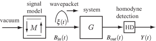
Figure 2: An ancilla system $M$ (a two-level system) is used as a signal model or ‘generating filter’. The ancilla system $M$ is driven by vacuum (quantum white noise), and produces a single-photon output. The cascade circuit illustrated in this figure is equivalent to the circuit of Fig. 1.

Specifically, we seek an ancilla system $M$ initialized in a state $|\gamma\rangle$ and driven by vacuum that provides a unitary dilation of the single photon driven system. This means that given our system $G=(S,L,H)$, can we find an ancilla system $M$ with state $|\gamma\rangle$ and an ancilla operator $R$ such that if $\tilde{U}(t)$ is the unitary for $\tilde{G}=G\triangleleft M$ then

$$\mathbb{E}_{\eta\xi}[X(t)]=\mathbb{E}_{\gamma\eta\phi}[\tilde{U}^{\ast}(t)(R\otimes X)\tilde{U}(t)].$$ (36)

Here, $X(t)=U^{\ast}(t)XU(t)$, where $U(t)$ is the unitary for $G$. Equation (36) means that the effect of the single photon field on the system is equivalent to the effect of the cascade of the ancilla on the system. The left hand side of (36) is a quantum expectation with respect to the state $|\eta\xi\rangle=|\eta\rangle\otimes|\xi\rangle$ with the field in the single photon state $|\xi\rangle$, while the right hand side involves quantum expectation in the extended system with respect to the initial state $|\gamma\eta\phi\rangle=|\gamma\rangle\otimes|\eta\rangle\otimes|\phi\rangle$, with the field in the vacuum state $|\phi\rangle$.

In order to fulfil the requirement (36), we consider the time derivative of both sides of (36) and determine the unknown signal model parameters by comparison. The time derivative of the left hand side of (36) is given by (21) or equations (III)-(26) above, while the right hand derivative can be computed from the Lindblad generator $\mathcal{G}_{G\triangleleft M}(A\otimes X)$ for the extended system $\tilde{G}=G\triangleleft M$,

$$\frac{d}{dt}\mathbb{E}_{\gamma\eta\phi}[\tilde{U}^{\ast}(t)(A\otimes X)\tilde{U}(t)]$$ (37)

$$= \mathbb{E}_{\gamma\eta\phi}[\tilde{U}^{\ast}(t)\mathcal{G}_{G\triangleleft M}(A\otimes X)\tilde{U}(t)],$$

where

$$\mathcal{G}_{G\triangleleft M}(A\otimes X) = A\otimes\mathcal{G}_{G}(X)+\mathcal{L}_{L_{0}}(A)\otimes X$$ (38)

$$+L^{\ast}_{0}A\otimes S^{\ast}[X,L]+AL_{0}\otimes[L^{\ast},X]S$$

$$+L_{0}^{\ast}L_{0}\otimes(S^{\ast}XS-X)$$

for any ancilla operator $A$ and system operator $X$.

Considering the definitions (22) of $\mu^{jk}_{t}(X)$ above, we must find ancilla operators $Q_{jk}$ and (non-vanishing) weighting functions $w_{jk}(t)$ such that

$$\mu^{jk}_{t}(X)=\frac{\tilde{\mu}_{t}(Q_{jk}\otimes X)}{w_{jk}(t)},$$ (39)

where

$$\tilde{\mu}_{t}(Q_{jk}\otimes X)=\mathbb{E}_{\gamma\eta\phi}[\tilde{U}^{\ast}(t)(Q_{jk}\otimes X)\tilde{U}(t)].$$ (40)

Now

$$\frac{d}{dt}\frac{\tilde{\mu}_{t}(Q_{jk}\otimes X)}{w_{jk}(t)} = \frac{\tilde{\mu}_{t}(\mathcal{G}_{G\triangleleft M}(Q_{jk}\otimes X))}{w_{jk}(t)}$$ (41)

$$-\frac{\tilde{\mu}_{t}(Q_{jk}\otimes X)}{w_{jk}(t)}\frac{\dot{w}_{jk}(t)}{w_{jk}(t)}.$$

Comparing this expression with equations (III)-(26) we find that (39) and (36) are satisfied if we choose the ancilla to be a two-level system with state $\gamma=|e_{1}\rangle$ (excited state), $R=Q_{11}=I$, $Q_{10}=\sigma_{-}$, $Q_{01}=\sigma_{+}$, $Q_{00}=n$, $w_{11}(t)=1$, $w_{10}(t)=w_{01}(t)=\sqrt{w(t)}$, $w_{00}(t)=w(t)=\int_{t}^{\infty}|\xi(s)|^{2}ds$, $L_{0}=\xi(t)\sigma_{-}/\sqrt{w(t)}$.

The signal model ancilla system is therefore

$$M=(I,\frac{\xi(t)\sigma_{-}}{\sqrt{w(t)}},0),$$ (42)

and so the extended system is

$$\tilde{G}=G\triangleleft M$$ (43)

$$=(S,L+\frac{\xi(t)}{\sqrt{w(t)}}S\sigma_{-},H+\frac{\xi(t)}{\sqrt{w(t)}}\mathrm{Im}(L^{\ast}S\sigma_{-})).$$

Remark. The output state of the generating filter $M$ can be understood as follows. If $V(t)$ denotes the unitary for $M$ driven by vacuum, and if the initial state is $|\psi(0)\rangle=|e_{1}\rangle\otimes|\phi\rangle$, then the state $|\psi(t)\rangle=V(t)|\psi(0)\rangle$ satisfies the Schrodinger equation

$$d|\psi(t)\rangle=\left[\frac{\xi(t)}{\sqrt{w(t)}}\sigma_{-}dB^{\ast}(t)-\frac{1}{2}\frac{|\xi(t)|^{2}}{w(t)}\sigma_{+}\sigma_{-}dt\right]\,|\psi(t)\rangle$$ (44)

(since $dB(t)|\phi\rangle=0$). It is an elementary calculation to see that this has the exact solution

$$|\psi(t)\rangle=\sqrt{w(t)}|e_{1}\otimes\phi\rangle+|e_{0}\otimes B_{t}^{-\ast}(\xi)\phi\rangle;$$ (45)

cf. (8). Since $\xi$ is square integrable, $|\psi(t)\rangle$ approaches the state $|e_{0}\otimes\xi\rangle$ as $t\to\infty$. Therefore the state of the field produced by the generating filter $M$ approaches the single photon state $|\xi\rangle$ asymptotically.

V Single Photon Filter

The quantum filter $\pi_{t}(X)=\mathbb{E}_{\eta\xi}[X(t)|Y(s),0\leq s\leq t]$ for the system $G$ driven by a single photon field may now be obtained from the quantum filter $\tilde{\pi}_{t}(A\otimes X)=\mathbb{E}_{\gamma\eta\phi}[\tilde{U}^{\ast}(t)(A\otimes X)\tilde{U}(t)|I\otimes Y(s),0\leq s\leq t]$ for the extended system $\tilde{G}=G\triangleleft M$ driven by vacuum [8], with the extended system parameters given by (43) (see the Appendix). Using the definition of conditional expectation (see [8] and the Appendix), it follows that

$$I\otimes\pi_{t}(X)=\tilde{\pi}_{t}(I\otimes X).$$ (46)

If we define

$$I\otimes\pi^{jk}_{t}(X)=\frac{\tilde{\pi}_{t}(Q_{jk}\otimes X)}{w_{jk}(t)},$$ (47)

we obtain the system of equations

$$d\pi^{11}_{t}(X)$$ (48)

$$= \bigl{(}\pi^{11}_{t}(\mathcal{G}(X))+\pi^{01}_{t}(S^{\ast}[X,L])\xi^{\ast}(t)$$

$$+\pi^{10}_{t}([L^{\ast},X]S)\xi(t)+\pi^{00}_{t}(S^{\ast}XS-X)|\xi(t)|^{2}\bigr{)}dt$$

$$+(\pi^{11}_{t}(XL+L^{\ast}X)+\pi^{01}_{t}(S^{\ast}X)\xi^{\ast}(t)+\pi^{10}_{t}(XS)\xi(t)$$

$$-\pi^{11}_{t}(X)\mathcal{K}_{t}(X))dW(t),$$

$$d\pi^{10}_{t}(X) = \bigl{(}\pi^{10}_{t}(\mathcal{G}(X))+\pi^{00}_{t}(S^{\ast}[X,L])\xi^{\ast}(t)\bigr{)}dt$$ (49)

$$+(\pi^{10}_{t}(XL+L^{\ast}X)+\pi^{00}_{t}(S^{\ast}X)\xi^{\ast}(t)$$

$$-\pi^{10}_{t}(X)\mathcal{K}_{t}(X))dW(t),$$

$$d\pi^{00}_{t}(X) = \pi^{00}_{t}(\mathcal{G}(X))dt+(\pi^{00}_{t}(XL+L^{\ast}X)$$ (50)

$$-\pi^{00}_{t}(X)\mathcal{K}_{t}(X))dW(t).$$

Here,

$$\mathcal{K}_{t}(X)=\pi^{11}_{t}(L+L^{\ast})+\pi^{01}_{t}(S)\xi(t)+\pi^{10}_{t}(S^{\ast})\xi^{\ast}(t)$$ (51)

and the innovations process $W(t)$ is a Wiener process with respect to the single photon state and is defined by

$$dW(t)=dY(t)-\mathcal{K}_{t}(X)dt.$$ (52)

We have $\pi^{01}_{t}(X)=\pi^{10}_{t}(X^{\ast})^{\ast}$, and the initial conditions are $\pi^{11}_{0}(X)=\pi^{00}_{0}(X)=\langle\eta,X\eta\rangle,\ \ \pi^{10}_{0}(X)=\pi^{01}_{0}(X)=0.$

Consequently the conditional expectation for the system driven by the single photon field is given by

$$\pi_{t}(X)=\mathbb{E}_{\eta\xi}[X(t)|Y(s),\ 0\leq s\leq t]=\pi^{11}_{t}(X),$$ (53)

and so the required quantum filter is given by the system of coupled equations (48)-(50).

Equations for the conditional density operators may easily be derived. Finally, we remark that although the master equations for systems driven by a single photon field have been obtained by other means in [13], to the best of our knowledge the quantum filtering (trajectory) equations for such systems have not been derived before.

VI Example

When the system is a two-level system or qubit, the filtering equations reduce to a finite set of stochastic differential equations. In this case we have $\mathfrak{H}_{S}=\mathbb{C}^{2}$. The system is specified by the parameters $S=I$, $L=\sqrt{\kappa}\,\sigma_{-}$, and $H=\omega\sigma_{z}$. Here $\kappa>0$ is a scalar parameter.

We begin with the master equations (30)-(33), and write

$$\rho^{00} = \frac{1}{2}(I+x^{00}\sigma_{x}+y^{00}\sigma_{y}+z^{00}\sigma_{z})$$ (54)

$$\rho^{01} = \frac{1}{2}(x^{01}\sigma_{x}+y^{01}\sigma_{y}+z^{01}\sigma_{z})=\rho^{10\ast}$$ (55)

$$\rho^{11} = \frac{1}{2}(I+x^{11}\sigma_{x}+y^{11}\sigma_{y}+z^{11}\sigma_{z})$$ (56)

Note that $x^{00}$, $y^{00}$, $z^{00}$ and $x^{11}$, $y^{11}$, $z^{11}$ are real, while $x^{01}$, $y^{01}$, $z^{01}$ may be complex. Also note, for example, $\rho^{00}(\sigma_{x})=x^{00},\ \ \rho^{01}(\sigma_{x})=x^{01\ast}$, etc. Then we obtain nine coupled equations for the nine coefficients:

$$\dot{x}^{00} =-2\omega y^{00}-\frac{\kappa}{2}x^{00},$$

$$\dot{y}^{00} =2\omega x^{00}-\frac{\kappa}{2}y^{00},$$

$$\dot{z}^{00} =-\kappa(1+z^{11}),$$

$$\dot{x}^{01} =-\frac{\kappa}{2}x^{01}-2\omega y^{01}-\sqrt{\kappa}\xi(t)^{*}z^{00},$$

$$\dot{y}^{01} =2\omega x^{01}-\frac{\kappa}{2}y^{01}-i\sqrt{\kappa}\xi(t)^{*}z^{00},$$

$$\dot{z}^{01} =-\kappa z^{01}-\sqrt{\kappa}x^{00}\xi(t)^{*}+i\sqrt{\kappa}y^{00}\xi(t)^{*},$$

$$\dot{x}^{11} =-\frac{\kappa}{2}x^{11}-2\omega y^{11}+\sqrt{\kappa}z^{01}\xi(t)+\sqrt{\kappa}z^{01*}\xi(t)^{*},$$

$$\dot{y}^{11} =2\omega x^{11}-\frac{\kappa}{2}y^{11}+i\sqrt{\kappa}z^{01}\xi(t)-i\sqrt{\kappa}z^{01*}\xi(t)^{*},$$

$$\dot{z}^{11} =-\kappa-\kappa z^{11}-\sqrt{\kappa}x^{01}\xi(t)-i\sqrt{\kappa}y^{01}\xi(t)$$

$$\ \ -\sqrt{\kappa}x^{01*}\xi(t)^{*}+i\sqrt{\kappa}y^{01*}\xi(t)^{*}.$$

For the quantum filter (48)-(50), we use a slightly more general representation for $\hat{\rho}^{jk}$ given by:

$$\hat{\rho}^{jk}=\frac{1}{2}(\hat{c}^{jk}I+\hat{x}^{jk}\sigma_{x}+\hat{y}^{jk}\sigma_{y}+\hat{z}^{jk}\sigma_{z}),$$

for $j,k=0,1$. Since $\langle\hat{\rho}^{11},I\rangle=1$ (i.e., $\hat{\rho}^{11}$ is a normalized conditional density operator), we always have that $\hat{c}^{11}=1$ at all times. However, unlike the master equation, this will not be so for $\hat{c}^{01},\hat{c}^{10},\hat{c}^{00}$, as these coefficients will evolve in time. This is the reason we need to consider the more general representation for $\hat{\rho}^{jk}$. The quantum filter for the two-level system is given by the finite set of coupled equations

$$d\hat{c}^{00} =(\sqrt{\kappa}\hat{x}^{00}$$

$$\ \ -(\sqrt{\kappa}\hat{x}^{11}+\frac{1}{2}\hat{c}^{01}\xi(t)+\frac{1}{2}\hat{c}^{01*}\xi(t)^{*})\hat{c}^{00})dW(t),$$

$$d\hat{x}^{00} =\bigl{(}-2\omega y^{00}-\frac{\kappa}{2}x^{00}\bigr{)}dt+\biggl{(}\sqrt{\kappa}\hat{c}^{00}$$

$$\ \ -(\sqrt{\kappa}\hat{x}^{11}+\frac{1}{2}\hat{c}^{01}\xi(t)+\frac{1}{2}\hat{c}^{01*}\xi(t)^{*})\hat{x}^{00}\biggr{)}dW(t),$$

$$d\hat{y}^{00} =\bigl{(}2\omega x^{00}-\frac{\kappa}{2}y^{00}\bigr{)}dt$$

$$\ \ -(\sqrt{\kappa}\hat{x}^{11}+\frac{1}{2}\hat{c}^{01}\xi(t)+\frac{1}{2}\hat{c}^{01*}\xi(t)^{*})\hat{y}^{00}\biggr{)}dW(t),$$

$$d\hat{z}^{00} =\bigl{(}-\kappa(1+z^{00}))dt+\biggl{(}\sqrt{\kappa}\hat{x}^{00}$$

$$\ \ -(\sqrt{\kappa}\hat{x}^{11}+\frac{1}{2}\hat{c}^{01}\xi(t)+\frac{1}{2}\hat{c}^{01*}\xi(t)^{*})\hat{z}^{00}\biggr{)}dW(t),$$

$$d\hat{c}^{01} =\biggl{(}\sqrt{\kappa}\hat{x}^{01}+\hat{c}^{00}\xi(t)^{*}$$

$$\ -(\sqrt{\kappa}\hat{x}^{11}+\frac{1}{2}\hat{c}^{01}\xi(t)+\frac{1}{2}\hat{c}^{01*}\xi(t)^{*})\hat{c}^{01}\biggr{)}dW(t),$$

$$d\hat{x}^{01} =\bigl{(}-\frac{\kappa}{2}x^{01}-2\omega y^{01}-\sqrt{\kappa}\xi(t)^{*}z^{00}\bigr{)}dt$$

$$\ \ +\biggl{(}\hat{x}^{00}\xi(t)^{*}+\sqrt{\kappa}\hat{c}^{01}$$

$$\ \ -(\sqrt{\kappa}\hat{x}^{11}+\frac{1}{2}\hat{c}^{01}\xi(t)+\frac{1}{2}\hat{c}^{01*}\xi(t)^{*})\hat{x}^{01}\biggr{)}dW(t),$$

$$d\hat{y}^{01} =\bigl{(}2\omega x^{01}-\frac{\kappa}{2}y^{01}-i\sqrt{\kappa}\xi(t)^{*}z^{00}\bigr{)}dt$$

$$\quad+\biggl{(}\hat{y}^{00}\xi(t)^{*}$$

$$\ \ -(\sqrt{\kappa}\hat{x}^{11}+\frac{1}{2}\hat{c}^{01}\xi(t)+\frac{1}{2}\hat{c}^{01*}\xi(t)^{*})\hat{y}^{01}\biggr{)}dW(t),$$

$$d\hat{z}^{01} =\bigl{(}-\kappa z^{01}-\sqrt{\kappa}x^{00}\xi(t)^{*}+i\sqrt{\kappa}y^{00}\xi(t)^{*}\bigr{)}dt$$

$$\quad+\biggl{(}\sqrt{\kappa}\hat{x}^{01}+\hat{z}^{00}\xi(t)^{*}$$

$$\ \ -(\sqrt{\kappa}\hat{x}^{11}+\frac{1}{2}\hat{c}^{01}\xi(t)+\frac{1}{2}\hat{c}^{01*}\xi(t)^{*})\hat{z}^{01}\biggr{)}dW(t),$$

$$d\hat{x}^{11} =\bigl{(}-\frac{\kappa}{2}x^{11}-2\omega y^{11}+\sqrt{\kappa}z^{01}\xi(t)+\sqrt{\kappa}z^{01*}\xi(t)^{*}\bigr{)}dt$$

$$\quad+\biggl{(}\sqrt{\kappa}+\hat{x}^{01*}\xi(t)^{*}+\hat{x}^{01}\xi(t)$$

$$\ \ -(\sqrt{\kappa}\hat{x}^{11}+\frac{1}{2}c^{01}\xi(t)+\frac{1}{2}c^{01*}\xi(t)^{*})\hat{x}^{11}\biggr{)}dW(t),$$

$$d\hat{y}^{11} =\bigl{(}2\omega x^{11}-\frac{\kappa}{2}y^{11}+i\sqrt{\kappa}z^{01}\xi(t)-i\sqrt{\kappa}z^{01*}\xi(t)^{*}\bigr{)}dt$$

$$\quad+\biggl{(}\hat{y}^{01*}\xi(t)^{*}+\hat{y}^{01}\xi(t)$$

$$\ \ -(\sqrt{\kappa}\hat{x}^{11}+\frac{1}{2}c^{01}\xi(t)+\frac{1}{2}c^{01*}\xi(t)^{*})\hat{y}^{11}\biggr{)}dW(t),$$

$$d\hat{z}^{11} =\bigl{(}-\kappa-\kappa z^{11}-\sqrt{\kappa}x^{01}\xi(t)-i\sqrt{\kappa}y^{01}\xi(t)$$

$$\ \ -\sqrt{\kappa}x^{01*}\xi(t)^{*}+i\sqrt{\kappa}y^{01*}\xi(t)^{*}\bigr{)}dt$$

$$\ \ +\biggl{(}\sqrt{\kappa}\hat{x}^{11}+\hat{z}^{01*}\xi(t)^{*}+\hat{z}^{01}\xi(t)$$

$$\ \ -(\sqrt{\kappa}\hat{x}^{11}+\frac{1}{2}c^{01}\xi(t)+\frac{1}{2}c^{01*}\xi(t)^{*})\hat{z}^{11}\biggr{)}dW(t).$$

The innovations process is given by

$$dW(t)=dY(t)-\bigl{(}\sqrt{\kappa}\,\hat{x}^{11}(t)+\hat{c}^{01}(t)\xi(t)+\hat{c}^{10}(t)\xi^{\ast}(t)\bigr{)}dt.$$ (57)

VII Discussion and Conclusion

In this paper we have derived the master equation and quantum filter for a class of open quantum systems that are coupled to single photon fields. The paper has focused on the case of quadrature measurements $Y(t)$ given by (14), (15). However, the methodology also applies to the case of counting measurements, corresponding to a photodetector in place of the homodyne detector in Figure 1.

The single photon filter consist of coupled equations that determine the evolution of the conditional state of the system under continuous (weak) measurement performed on the output field, in contrast to the familiar single filtering equation for open Markov quantum systems that are coupled to coherent boson fields. This coupled equations structure of the master and filter equations is a reflection of the non-Markov nature of systems coupled to single photon fields. Indeed, a key feature of our approach is the embedding of the system into a larger extended system, a technique often employed in the analysis of non-Markov systems, providing an elegant framework within which to study the the dynamics, both unconditional and conditional, of the system. We expect that the basic approach taken in this paper can be adapted to study quantum systems that are coupled to other types of highly non-classical boson fields.

The quantum filter for a system $G=(S,L,H)$ (driven by vacuum) for the quadrature output field observable $Y(t)$ (given by (14)) is

$$d\pi_{t}(X)=\pi_{t}(\mathcal{G}_{G}(X))dt$$ (58)

$$+(\pi_{t}(XL+L^{\ast}X)-\pi_{t}(L+L^{\ast})\pi_{t}(X))dW(t),$$

where $W(t)$, a Wiener process called the innovations process, is given by $dW(t)=dY(t)-\pi_{t}(L+L^{\ast})dt).$ By the spectral theorem it follows that the quantum filter is equivalent to a classical system driven by the measurement record, [7, 8]. Perhaps the simplest way to derive the quantum filter is to use the conditional characteristic function, [5, 7, 25], which we now briefly summarize.

We begin with a short discussion of quantum conditional expectation. The measurement signal $Y(s)$, $0\leq s\leq t$, is a collection of commuting self-adjoint operators. These operators form a subspace $\mathscr{Y}_{t}$ in the space of operators, and the quantum conditional expectation $\mathbb{E}_{\eta\phi}[X(t)|Y(s)$, $0\leq s\leq t]$ is the orthogonal projection of the system operator $X(t)$ at time $t$ (since the field serves as a probe, we have the commutation relation $[X(t),Y(s)]=0$ for all $0\leq s\leq t$ (non-demolition), and so the conditional expectation is well-defined). The orthogonal projection property corresponds to least squares estimation, and leads to the following characterization (17) mentioned in Section II. We will use this characterization in the following form. Define, for any function $g$,

$$c_{g}(t)=\exp\{\int_{0}^{t}g(s)dY(s)-\frac{1}{2}\int_{0}^{t}|g(s)|^{2}ds\},$$ (59)

and note $dc_{g}(t)=g(t)c_{g}(t)dY(t)$. Then we require

$$\mathbb{E}_{\eta\phi}[X(t)c_{g}(t)]=\mathbb{E}_{\eta\phi}[\hat{X}(t)c_{g}(t)],$$ (60)

for all functions $g$.

Now suppose that $d\hat{X}(t)$ has the form

$$d\hat{X}(t)=\alpha(t)dt+\beta(t)dY(t),$$ (61)

where $\alpha$ and $\beta$ are to be determined from the relation (60). Now using the QSDE (11) for $X(t)=j_{t}(X)$, we have

$$\frac{d}{dt}\mathbb{E}_{\eta\phi}[X(t)c_{g}(t)]$$

$$=\mathbb{E}_{\eta\phi}[c_{g}(t)\pi_{t}(-i[X,H]+\mathcal{G}_{L}(X))$$

$$+g(t)c_{g}(t)\pi_{t}(XL+L^{\ast}X)]$$ (62)

(here we have used property (60)). Similarly, using (61) we have

$$\frac{d}{dt}\mathbb{E}_{\eta\phi}[\hat{X}(t)c_{g}(t)]$$

$$=\mathbb{E}_{\eta\phi}[c_{g}(t)(\alpha(t)+\pi_{t}(L+L^{\ast})\beta(t))$$

$$+g(t)c_{g}(t)(\beta(t)+\pi_{t}(L+L^{\ast})\hat{X}(t)]$$ (63)

Now equating the RHS of (62) and (63) and using the fact that $g$ is arbitrary we find that

$$\alpha(t) = \pi_{t}(-i[X,H]+\mathcal{G}_{L}(X))-\pi_{t}(L+L^{\ast})\beta(t)$$

$$\beta(t) = \pi_{t}(XL+L^{\ast}X)-\pi_{t}(L+L^{\ast})\pi_{t}(X)$$

The quantum filter (58) now follows from this.

References

• [1] G. Auletta, M. Fortunato, and G. Parisi. Quantum Mechanics. Cambridge University Press, Cambridge, UK, 2009.
• [2] H.A. Bachor and T.C. Ralph. A Guide to Experiments in Quantum Optics. Wiley-VCH, Weinheim, Germany, second edition, 2004.
• [3] A. Barchielli. Continual measurements in quantum mechanics, Summer School on Quantum Open Systems 2003.
• [4] A. Barchielli and V.P. Belavkin. Measurements continuous in time and a posteriori states in quantum mechanics. J. Phys. A: Math. Gen., 24:1495–1514, 1991.
• [5] V.P. Belavkin. Quantum continual measurements and a posteriori collapse on CCR. Commun. Math. Phys., 146:611–635, 1992.
• [6] V.P. Belavkin. Quantum stochastic calculus and quantum nonlinear filtering. J. Multivariate Analysis, 42:171–201, 1992.
• [7] V.P. Belavkin. Quantum diffusion, measurement, and filtering. Theory Probab. Appl., 38(4):573–585, 1994.
• [8] L. Bouten, R. van Handel, and M.R. James. An introduction to quantum filtering. SIAM J. Control and Optimization, 46(6):2199–2241, 2007.
• [9] H.P. Breuer. Genuine quantum trajectories for non-Markovian processes. Phys. Rev. A, 70:012106, 2004.
• [10] H. Carmichael. An Open Systems Approach to Quantum Optics. Springer, Berlin, 1993.
• [11] C.W. Gardiner and M.J. Collett. Input and output in damped quantum systems: Quantum stochastic differential equations and the master equation. Phys. Rev. A, 31(6):3761–3774, 1985.
• [12] C.W. Gardiner and P. Zoller. Quantum Noise. Springer, Berlin, 2000.
• [13] K. Gheri, K. Ellinger, T. Pellizzari, and P. Zoller, Photon-wavepackets as flying quantum bits, Fortschr. Phys., 46 (1998), pp. 401–415.
• [14] N. Gisin, G. Ribordy, W. Tittel, and H. Zbinden. Quantum cryptography. Reviews of Modern Physics, 74(1):145, 2002.
• [15] J. Gough and M.R. James. The series product and its application to quantum feedforward and feedback networks. IEEE Trans. Automatic Control, 54(11):2530–2544, 2009.
• [16] F. Grosshans and P. Grangier. Effective quantum efficiency in the pulsed homodyne detection of a n-photon state. Eur. Phys. J. D, 14:119–125, 2001.
• [17] R.L. Hudson and K.R. Parthasarathy. Quantum Ito’s formula and stochastic evolutions. Commun. Math. Phys., 93:301–323, 1984.
• [18] E. Knill, R. Laflamme, and G.J. Milburn. A scheme for efficient quantum computation with linear optics. Nature, 409:46–52, 2001.
• [19] R. Loudon. The Quantum Theory of Light. Oxford University Press, Oxford, 3rd edition, 2000.
• [20] X. Maitre, E. Hagley, G. Nogues, C. Wunderlich, P. Goy, M. Brune, J.M. Raimond, and S. Haroche. Quantum memory with a single photon in a cavity. Phys. Rev. Lett., 79(4):769–772, 1997.
• [21] E. Merzbacher. Quantum Mechanics. Wiley, New York, third edition, 1998.
• [22] G. J. Milburn. Quantum optics. In F. Träger, editor, Springer Handbook of Lasers and Optics, chapter 14, pages 1053–1078. Springer, 2007.
• [23] G. J. Milburn. Coherent control of single photon states. Eur. Phys. J. Special Topics, 159:113–117, 2008.
• [24] K.R. Parthasarathy. An Introduction to Quantum Stochastic Calculus. Birkhauser, Berlin, 1992.
• [25] R. van Handel, J. Stockton, and H. Mabuchi. Feedback control of quantum state reduction. IEEE Trans. Automatic Control, 50:768–780, 2005.
• [26] J. Volz, M. Weber, D. Schlenk, W. Rosenfeld, J. Vrana, K. Saucke, C. Kurtsiefer, and H. Weinfurter. Observation of entanglement of a single photon with a trapped atom. Phys. Rev. Lett., 96:030404, 2006.
• [27] H. Wiseman and G.J. Milburn. Quantum theory of field-quadrature measurements. Phys. Rev. A, 47(1):642–663, 1993.
• [28] H.M. Wiseman and G.J. Milburn. Quantum Measurement and Control. Cambridge University Press, Cambridge, UK, 2010.