Quantum Filtering for Systems Driven by Fields in Single Photon States and Superposition of Coherent States using Non-Markovian Embeddings

Abstract

The purpose of this paper is to determine quantum master and filter equations for systems coupled to fields in certain non-classical continuous-mode states. Specifically, we consider two types of field states (i) single photon states, and (ii) superpositions of coherent states. The system and field are described using a quantum stochastic unitary model. Master equations are derived from this model and are given in terms of systems of coupled equations. The output field carries information about the system, and is continuously monitored. The quantum filters are determined with the aid of an embedding of the system into a larger non-Markovian system, and are given by a system of coupled stochastic differential equations.

Keywords: quantum filtering, continuous-mode single photon states, continuous-mode superpositions of coherent states, quantum stochastic processes

1 Introduction

In recent years single photon states of light and superpositions of coherent states have become increasingly important due to applications in quantum technology, in particular, quantum computing and quantum information systems, [25], [27], [23], [18], [30]. For instance, the light may interact with a system, say an atom, quantum dot, or cavity, and this system may be used as a quantum memory, [25], or to control the pulse shape of the single photon state [27]. When light interacts with a quantum system, information about the system is contained in the scattered light. This information may be useful for monitoring the behavior of the system, or for controlling it. The topic of this paper concerns the extraction of information from the scattered light when the incoming light is placed in a single photon state $|\Psi\rangle=|1_{\xi}\rangle$, or a superposition of coherent states $|\Psi\rangle=\sum_{j}\alpha_{j}|f_{j}\rangle$, as illustrated in Figure 1.

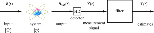
Figure 1: A system initialized in a state $|\eta\rangle$ coupled to a field in a state $|\Psi\rangle$ (single photon or superposition of coherent states). The output field is continuously monitored by homodyne detection (assumed perfect) to produce a classical measurement signal $Y(t)$. The output $Y(t)$ is filtered to produce estimates $\hat{X}(t)=\pi_{t}(X)$ of system operators $X$ at time $t$.

The problem of extracting information from continuous measurement of the scattered light is a problem of quantum filtering, [4], [5], [6], [11], [31], [3], [9], [32]. The current state of the art for quantum filtering considers incoming light in a vacuum or other Gaussian state, with quadrature or counting measurements. Both single photon states of light, and superpositions of coherent states of light, are highly non-classical, and are fundamentally different from Gaussian states. In view of the increasing importance of these non-Gaussian states of light, the purpose of this paper is to solve a quantum filtering problem for systems driven by fields in single photon states and superpositions of coherent states.

In the case of single photon fields, the master equation describing unconditional dynamics was shown to be a system of coupled equations in [17], a feature of non-Markovian character. Markovian embeddings were used in [10] to derive quantum trajectory equations (quantum filtering equations) for a class of non-Markovian master equations. In recent work, the authors have shown how to construct ancilla systems to combine with the system of interest to form a Markovian extended system driven by vacuum from which quantum filtering results may be obtained for single photon states and superpositions of coherent states from the standard filter for the extended system, [19], [20]. However, depending on the complexity of the non-classical state, it may possibly be difficult to determine suitable ancilla systems, and indeed the superposition case was not straightforward. In this paper we present an alternative approach to the embedding that also allows for the derivation of the quantum filter. The extended system forms a non-Markovian system, with the ancilla, system and field initialized in a superposition state. While standard filtering results do not apply, the quantum stochastic methods can nevertheless be applied to determine the quantum filters. In this way, we expand the range of methods that may be applied to derive quantum filters for non-classical states.

The paper is organized as follows. In section 2 the idealized filtering problem to be solved in this paper is formulated. The continuous mode single photon states are defined in Section 3.1. The master equation for the single photon field state is derived in Section 3.2 using the model presented in Section 2. This leads naturally to Section 3.3, where the system is embedded in a larger model, inspired by the approach used in [10] but differing in the details. This extended system provides a compact and transparent description of the problem, and may readily be generalized to $n$-photon states, and indeed, multiple channels of $n$-photon states. The quantum filter for the extended system is presented in Section 3.4, with a derivation extending the reference method appearing in Section 3.6. The filtering results for the extended system are used to find the filtering equations for the original problem involving a single photon field in Section 3.5. The superposition of coherent field states is defined in Section 4.1, and a suitable embedded system for this case is described in Section 4.2. The corresponding master and filtering equations are presented in Sections 4.3 and 4.4, respectively. Some concluding remarks are made in Section 5.

In this paper we are not concerned with technical issues concerning domains of unbounded operators and related matters, and indeed, we assume that the system operators are bounded, and that all quantum stochastic integrals are well-defined in the sense of Hudson-Parthasarathy, [22].

Notation: We use the standard Dirac notation $|\psi\rangle$ to denote state vectors (vectors in a Hilbert space) [26], [1]. The superscript ^∗ indicates Hilbert space adjoint or complex conjugate. The inner product of state vectors $|\psi_{1}\rangle$ and $|\psi_{2}\rangle$ is denoted $\langle\psi_{1}|\psi_{2}\rangle$. The expected value of an operator $X$ when the system is in state $|\psi\rangle$ is denoted $\mathbb{E}_{\psi}[X]=\langle\psi|X|\psi\rangle$. For operators $A$ and $B$ we write $\langle A,B\rangle=\mathrm{tr}[A^{\ast}B].$

2 Problem Formulation

We consider a quantum system $S$ coupled to a quantum field $B$, as shown in Figure 1. The field $B$ has two components, the input field $B_{in}$ and the output field, $B_{out}$. In this paper we consider two non-classical cases for the state $|\Psi\rangle$ of the input field (i) a single photon state $|\Psi\rangle=|1_{\xi}\rangle$, where $\xi$ is a complex valued function such that $\int_{0}^{\infty}|\xi(s)|^{2}ds=1$ (representing the wave packet shape), or (ii) a superposition of coherent states $|\Psi\rangle=\sum_{j}\alpha_{j}|f_{j}\rangle$, where $|f_{j}\rangle$ are coherent states and the complex numbers $\alpha_{j}$ ($j=1,\ldots,n$) are normalized weights.

As illustrated in Figure 1, the field interacts with the quantum system $S$, and the results of this interaction provide information about the system that may be obtained through continuous measurement of an observable $Y(t)$ of the output field $B_{out}(t)$. The filtering problem of interest in this paper is to determine the conditional state from which estimates $\hat{X}(t)$ of system operators $X$ may be determined at time $t$ based on knowledge of the observables $\{Y(s)$, $0\leq s\leq t\}$.

In what follows the system $S$ is assumed to be defined on a Hilbert space $\mathfrak{H}_{S}$, with an initial state denoted $|\eta\rangle\in\mathfrak{H}_{S}$. The input field $B_{in}$ is described in terms of annihilation $B(\xi)$ and creation $B^{\ast}(\xi)$ operators defined on a Fock space $\mathfrak{F}$, [28, Chapter II], [9, Section 4]. Quantum expectation will be denoted by the symbol $\mathbb{E}$, and when we wish to display the underlying state, we employ subscripts; for example, $\mathbb{E}_{\eta\Psi}$ denotes quantum expectation with respect to the state $|\eta\rangle\otimes|\Psi\rangle$.

The dynamics of the system will be described using the quantum stochastic calculus, [22], [15], [28], [16], [9]. Quantum stochastic integrals are defined in terms of fundamental field operators $B(t)$, $B^{\ast}(t)$ and $\Lambda(t)$, [28, Chapter II], [9, Section 4]. The non-zero Ito products for the field operators are

$$dB(t)dB^{\ast}(t)=dt,\ \ dB(t)d\Lambda(t)=dB(t),\ \ d\Lambda(t)d\Lambda(t)=d\Lambda(t),\ \ d\Lambda(t)dB^{\ast}(t)=dB^{\ast}(t).$$ (1)

The dynamics of the composite system is described by a unitary $U(t)$ solving the Schrödinger equation, or quantum stochastic differential equation (QSDE),

$$dU(t)=\{(S-I)d\Lambda(t)+LdB^{\ast}(t)-L^{\ast}SdB(t)-(\frac{1}{2}L^{\ast}L+iH)dt\}U(t),$$ (2)

with initial condition $U(0)=I$. Here, $H$ is a fixed self-adjoint operator representing the free Hamiltonian of the system, and $L$ and $S$ are system operators determining the coupling of the system to the field, with $S$ unitary. In this paper, for simplicity we assume that the parameters $S,L,H$ are bounded operators on the system Hilbert space $\mathfrak{H}_{S}$. However, we remark under some suitable additional conditions the results and equations obtained in this paper should also be extendable to some special classes of QSDEs with unbounded parameters, exploiting the results in [13, 14].

A system operator $X$ at time $t$ is given in the Heisenberg picture by $X(t)=j_{t}(X)=U(t)^{\ast}(X\otimes I)U(t)$ and it follows from the quantum Ito calculus that

$$dj_{t}(X) = j_{t}(S^{\ast}XS-X)d\Lambda(t)+j_{t}(S^{\ast}[X,L])dB(t)^{\ast}$$ (3)

$$+j_{t}([L^{\ast},X]S)dB(t)+j_{t}(\mathcal{L}(X))dt,$$

where

$$\mathcal{L}(X)=\frac{1}{2}L^{\ast}[X,L]+\frac{1}{2}[L^{\ast},X]L-i[X,H].$$ (4)

The map $X\mapsto\mathcal{L}(X)$ is known as the Lindblad generator, while the quartet of maps $X\mapsto\mathcal{L}(X),S^{\ast}XS-X,\,S^{\ast}[X,L],\,[L^{\ast},X]S$ are known as Evans-Hudson maps.

The output field is defined by $B_{out}(t)=U(t)^{\ast}B(t)U(t)$. In this paper we consider the output field observable $Y(t)$ defined by

$$Y(t)=U(t)^{\ast}Z(t)U(t),$$ (5)

where

$$Z(t)=B(t)+B^{\ast}(t),$$ (6)

is a quadrature observable of the input field (the counting case $Z(t)=\Lambda(t)$ is discussed briefly in Section 5). Note that both $Z(t)$ and $Y(t)$ are self-adjoint and self-commutative: $[Z(t),Z(s)]=0$ and $[Y(t),Y(s)]=0$. We write $\mathscr{Z}_{t}$ and $\mathscr{Y}_{t}$ for the subspaces of commuting operators generated by the observables $Z(s)$, $Y(s)$, $0\leq s\leq t$, respectively. They are related by the unitary rotation $\mathscr{Y}_{t}=U(t)^{\ast}\mathscr{Z}_{t}U(t)$. Physically, $Y(t)$ may represent the integrated photocurrent arising in an idealized (perfect) homodyne photodetection scheme, as in Figure 1. For further information on homodyne detection, we refer the reader to the literature; for example, [2], [3], [32].

The primary goal of this paper is to determine the quantum filter for the quantum conditional expectation (see, e.g. [9, Definition 3.13])

$$\hat{X}(t)=\mathbb{E}_{\eta\Psi}[X(t)\,|\,\mathscr{Y}_{t}].$$ (7)

This conditional expectation is well defined, since $X(t)$ commutes with the subspace $\mathscr{Y}_{t}$ (non-demolition condition). The conditional estimate $\hat{X}(t)$ is affiliated to $\mathscr{Y}_{t}$ (written in abbreviated fashion as $\hat{X}(t)\in\mathscr{Y}_{t}$) and is characterized by the requirement that

$$\mathbb{E}_{\eta\Psi}[\hat{X}(t)K]=\mathbb{E}_{\eta\Psi}[X(t)K]$$ (8)

for all $K\in\mathscr{Y}_{t}$.

3 Single Photon Input Fields

3.1 Single Photon Fields States

In this section we consider the continuous-mode single photon state $|\Psi\rangle=|1_{\xi}\rangle$ defined by [24, sec. 6.3], [27, eq. (9)]

$$|1_{\xi}\rangle=B^{\ast}(\xi)|0\rangle,$$ (9)

where $\xi$ is a complex valued function such that $\int_{0}^{\infty}|\xi(s)|^{2}ds=1$, and $|0\rangle$ is the vacuum state of the field. Expression (9) says that the single photon wavepacket with temporal shape $\xi$ is created from the vacuum using the field operator $B^{\ast}(\xi)$.

The Hilbert space for the composite system is

$$\mathfrak{H}=\mathfrak{H}_{S}\otimes\mathfrak{F}=\mathfrak{H}_{S}\otimes\mathfrak{F}_{t]}\otimes\mathfrak{F}_{(t},$$

where here we have exhibited the continuous temporal tensor product decomposition of the Fock space $\mathfrak{F}=\mathfrak{F}_{t]}\otimes\mathfrak{F}_{(t}$ into past and future components, which is of basic importance in what follows. Write

$$\mathbb{E}_{11}[X\otimes F]=\langle\eta 1_{\xi}|(X\otimes F)|\eta 1_{\xi}\rangle=\langle\eta|X|\eta\rangle\langle 1_{\xi}|F|1_{\xi}\rangle$$ (10)

for the expectation with respect to the product state $|\eta 1_{\xi}\rangle$, where the field is in the single photon state. Here and in what follows $X$ is a bounded system operator acting on $\mathfrak{H}_{S}$, and $F$ is a field operator acting on the Fock space $\mathfrak{F}$. Similarly, we may define the expectation when the field is in the vacuum state,

$$\mathbb{E}_{00}[X\otimes F]=\langle\eta 0|(X\otimes F)|\eta 0\rangle=\langle\eta|X|\eta\rangle\langle 0|F|0\rangle.$$ (11)

We will also have need for the cross-expectations

$$\mathbb{E}_{10}[X\otimes F]=\langle\eta 1_{\xi}|(X\otimes F)|\eta 0\rangle,\ \text{and}\ \mathbb{E}_{01}[X\otimes F]=\langle\eta 0|(X\otimes F)|\eta 1_{\xi}\rangle.$$ (12)

A crucial difference between the single photon state and the vacuum state is that the later state factorizes $|0\rangle=|0_{t]}\rangle\otimes|0_{(t}\rangle$ with respect to the temporal factorization $\mathfrak{F}=\mathfrak{F}_{t]}\otimes\mathfrak{F}_{(t}$ of the Fock space, with $|0_{t]}\rangle\in\mathfrak{F}_{t]}$ and $|0_{(t}\rangle\in\mathfrak{F}_{(t}$, while the former does not. Rather, we have

$$|1_{\xi}\rangle=B^{\ast}(\xi)|0\rangle=|{1_{\xi}}_{t]}\rangle\otimes|0_{(t}\rangle+|0_{t]}\rangle\otimes|{1_{\xi}}_{(t}\rangle,$$ (13)

where

$$|{1_{\xi}}_{t]}\rangle=B^{-\ast}_{t}(\xi)|0_{t]}\rangle,\ \text{and}\ |{1_{\xi}}_{(t}\rangle=B^{+\ast}_{t}(\xi)|0_{(t}\rangle,$$ (14)

and

$$B^{-}_{t}(\xi)=B(\xi\chi_{[0,t]}),\ \ B^{+}_{t}(\xi)=B(\xi\chi_{(t,\infty]}),\ \ B(\xi)=B^{-}_{t}(\xi)+B^{+}_{t}(\xi).$$ (15)

Here, $\chi_{[0,t]}$ is the indicator function for the time interval $[0,t]$. Note that while $|1_{\xi}\rangle$ has unit norm, we have

$$\parallel|{1_{\xi}}_{t]}\rangle\parallel^{2}=\int_{0}^{t}|\xi(s)|^{2}ds,\ \text{and}\ \parallel|{1_{\xi}}_{(t}\rangle\parallel^{2}=\int_{t}^{\infty}|\xi(s)|^{2}ds.$$ (16)

A consequence of the additive decomposition (13) and the definitions (15) is the following. Let $K(t)$ be a bounded operator acting on the full Hilbert space $\mathfrak{H}$ that is adapted, i.e. $K(t)$ acts trivially on $\mathfrak{F}_{(t}$, the field in the future. Then the expectation with respect to the single photon field may be expressed in terms of the vacuum state as follows:

$$\mathbb{E}_{11}[K(t)] = \mathbb{E}_{00}[B^{-}_{t}(\xi)K(t)B^{-\ast}_{t}(\xi)+r(t)K(t)]$$ (17)

where $r(t)=\int_{t}^{\infty}|\xi(s)|^{2}ds$.

3.2 Master Equation

Before deriving the quantum filter, we work out dynamical equations for the unconditioned single photon expectation, [17]. To assist us in evaluating this expectation, we make use of the following lemma.

Lemma 3.1

Let $K(t)$ be a bounded quantum stochastic process defined by

$$K(t)=\int_{0}^{t}M_{0}(s)ds+\int_{0}^{t}M_{-}(s)dB(s)+\int_{0}^{t}M_{+}(s)dB^{\ast}(s)+\int_{0}^{t}M_{1}(s)d\Lambda(s),$$ (18)

where $M_{0}$, $M_{\pm}$ and $M_{1}$ are bounded and adapted. Then we have

$$\mathbb{E}_{11}[K(t)] = \mathbb{E}_{11}[\int_{0}^{t}M_{0}(s)ds]+\mathbb{E}_{10}[\int_{0}^{t}M_{-}(s)\xi(s)ds]$$ (19)

$$+\mathbb{E}_{01}[\int_{0}^{t}M_{+}(s)\xi^{\ast}(s)ds]+\mathbb{E}_{00}[\int_{0}^{t}M_{1}(s)|\xi(s)|^{2}ds],$$

$$\mathbb{E}_{10}[K(t)] = \mathbb{E}_{10}[\int_{0}^{t}M_{0}(s)ds]+\mathbb{E}_{00}[\int_{0}^{t}M_{+}(s)\xi^{\ast}(s)ds],$$ (20)

$$\mathbb{E}_{01}[K(t)] = \mathbb{E}_{01}[\int_{0}^{t}M_{0}(s)ds]+\mathbb{E}_{00}[\int_{0}^{t}M_{-}(s)\xi(s)ds],$$ (21)

$$\mathbb{E}_{00}[K(t)] = \mathbb{E}_{00}[\int_{0}^{t}M_{0}(s)ds].$$ (22)

Proof.    Using (17), the expressions $B^{-}_{t}(\xi)=\int_{0}^{t}\xi^{\ast}(s)dB(s)$, $B^{-\ast}_{t}(\xi)=\int_{0}^{t}\xi(s)dB^{\ast}(s)$, and the Ito rule we have

$$\mathbb{E}_{11}[dK(t)] = \mathbb{E}_{00}[d(B^{-}_{t}(\xi)K(t)B^{-\ast}_{t}(\xi)+r(t)K(t))]$$ (23)

$$= \mathbb{E}_{00}[B^{-}_{t}(\xi)M_{0}(t)B^{-\ast}_{t}(\xi)+r(t)M_{0}(t)$$

$$+M_{+}(t)B^{-\ast}_{t}(\xi)\xi^{\ast}(t)+B^{-}_{t}(\xi)M_{-}(t)\xi(t)+M_{1}(t)|\xi(t)|^{2}]dt$$

$$= \mathbb{E}_{11}[M_{0}(t)]dt+\mathbb{E}_{00}[M_{+}(t)B^{\ast}(\xi)\xi^{\ast}(t)+B(\xi)M_{-}(t)\xi(t)+M_{1}|\xi(t)|^{2}]dt.$$

This last line is justified since $M_{\pm}$ are adapted and $\mathbb{E}_{00}[B^{+}_{t}(\xi)]=0$. That is,

$$\mathbb{E}_{11}[dK(t)]=\mathbb{E}_{11}[M_{0}(t)]dt+\mathbb{E}_{01}[M_{+}(t)]\xi^{\ast}(t)dt+\mathbb{E}_{10}[M_{-}(t)]\xi(t)dt+\mathbb{E}_{00}[\int_{0}^{t}M_{1}(s)|\xi(s)|^{2}ds].$$ (24)

This proves (19). The remaining expressions are proven in a similar manner. $\Box$

We will first express the master equation in Heisenberg form using the expectations

$$\mu^{jk}_{t}(X)=\mathbb{E}_{jk}[X(t)].$$ (25)

Note that for all $t\geq 0$ we have

$$\mu_{t}^{00}(I)=1=\mu^{11}_{t}(I),\ \ \ \mu^{01}_{t}(I)=0=\mu^{10}_{t}(I).$$ (26)

Theorem 3.2

The master equation in Heisenberg form for the system when the field is in the single photon state $|1_{\xi}\rangle$ is given by the system of equations

$$\dot{\mu}^{11}_{t}(X) = \mu^{11}_{t}(\mathcal{L}(X))+\mu^{01}_{t}(S^{\ast}[X,L])\xi^{\ast}(t)+\mu^{10}_{t}([L^{\ast},X]S)\xi(t)$$ (27)

$$+\mu^{00}_{t}(S^{\ast}XS-S)|\xi(t)|^{2},$$

$$\dot{\mu}^{10}_{t}(X) = \mu^{10}_{t}(\mathcal{L}(X))+\mu^{00}_{t}(S^{\ast}[X,L])\xi^{\ast}(t),$$ (28)

$$\dot{\mu}^{01}_{t}(X) = \mu^{01}_{t}(\mathcal{L}(X))+\mu^{00}_{t}([L^{\ast},X]S)\xi(t),$$ (29)

$$\dot{\mu}^{00}_{t}(X) = \mu^{00}_{t}(\mathcal{L}(X)).$$ (30)

The initial conditions are

$$\mu^{11}_{0}(X)=\mu^{00}_{0}(X)=\langle\eta,X\eta\rangle,\ \ \mu^{10}_{0}(X)=\mu^{01}_{0}(X)=0.$$ (31)

Proof.    Equations (27)- (30) are obtained by applying Lemma 3.1 to the Heisenberg equation (3). $\Box$

It is apparent from Theorem 3.2 that the single photon expectation $\mu^{11}_{t}(X)=\mathbb{E}_{11}[X(t)]$ cannot be determined by a single differential equation, and that instead a system of coupled equations is required, equation (27)-(30). Note that the unitary matrix $S$ appearing in the Schrödinger equation (2) does appear in the single photon master equations (27)-(30), in contrast to the vacuum case (which corresponds to (30)).

3.3 Embedding

In this section we construct a suitable embedding for the system and single photon field, and show how the system of master equations from Section 3.2 can be compactly represented as a single equation for a larger system. This embedding will be used in subsequent sections to derive the quantum filter. We should emphasize, however, that our embedding is not the same as that used in [10], [19], [20]. The embedding is illustrated in Figure 2.

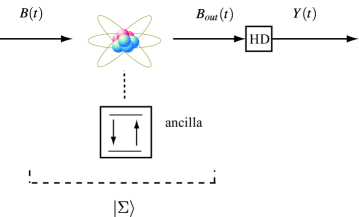
Figure 2: System embedded in the extended system. While the analysis does not employ any coupling between the system and ancilla two-level system, the ancilla, system and field are assumed to be initialized in a superposition state $|\Sigma\rangle$ defined in equation (36).

Recall that the system and field are defined on a Hilbert space $\mathfrak{H}=\mathfrak{H}_{S}\otimes\mathfrak{F}$. We define an extended space

$$\tilde{\mathfrak{H}}=\mathbb{C}^{2}\otimes\mathfrak{H}=\mathfrak{H}\oplus\mathfrak{H}$$ (32)

which includes the system, field and an ancilla two-level system. Let $|e_{0}\rangle$ and $|e_{1}\rangle$ be an orthonormal basis for $\mathbb{C}^{2}$,

$$|e_{0}\rangle=\left[\begin{array}[]{c}0\\ 1\end{array}\right],\ \ |e_{1}\rangle=\left[\begin{array}[]{c}1\\ 0\end{array}\right],$$ (33)

and let $A$ be an operator acting on $\mathbb{C}^{2}$, i.e. a complex $2\times 2$ matrix

$$A=\left[\begin{array}[]{cc}a_{11}&a_{10}\\ a_{01}&a_{00}\end{array}\right].$$ (34)

It may be helpful to think of operators $A\otimes X\otimes F$ on the extended space $\tilde{\mathfrak{H}}$ represented in the Kronecker product form

$$A\otimes(X\otimes F)=\left[\begin{array}[]{cc}a_{11}(X\otimes F)&a_{10}(X\otimes F)\\ a_{01}(X\otimes F)&a_{00}(X\otimes F)\end{array}\right].$$ (35)

We allow the extended system to evolve unitarily according to $I\otimes U(t)$, where $U(t)$ is the unitary operator for the system and field, given by the Schrödinger equation (2). Note in particular that the system is not coupled to the ancilla $\mathbb{C}^{2}$, and observables of this two-level system are static. We initialize the extended system in the superposition state

$$|\Sigma\rangle=\alpha_{1}|e_{1}\eta 1_{\xi}\rangle+\alpha_{0}|e_{0}\eta 0\rangle,$$ (36)

where $|\alpha_{0}|^{2}+|\alpha_{1}|^{2}=1$. This state evolves according to

$$|\Sigma(t)\rangle=(I\otimes U(t))|\Sigma\rangle.$$ (37)

For notational convenience we write

$$w_{jk}=\alpha_{j}^{\ast}\alpha_{k}$$ (38)

and note that $w=\sum_{jk}w_{jk}|e_{j}\rangle\langle e_{k}|$ is a density matrix for $\mathbb{C}^{2}$.

The expectation with respect to the superposition state $|\Sigma\rangle$ is given by

$$\tilde{\mu}_{t}(A\otimes X)=\mathbb{E}_{\psi}[A\otimes X(t)]=\langle\Sigma|(A\otimes X(t))|\Sigma\rangle=\sum_{jk}w_{jk}a_{jk}\mu^{jk}_{t}(X).$$ (39)

This expectation is correctly normalized, $\mu_{t}(I\otimes I)=1$, and the expectations $\mu^{jk}_{t}(X)$ defined in Section 3.2 are scaled components of $\tilde{\mu}_{t}(A\otimes X)$:

$$\mu^{jk}_{t}(X)=\frac{\tilde{\mu}_{t}(|e_{j}\rangle\langle e_{k}|\otimes X)}{w_{jk}},$$ (40)

for $w_{jk}\neq 0$, otherwise it can be set to, say, 0. We also have

$$\mu^{jk}_{t}(X)=\frac{w_{11}\tilde{\mu}_{t}(|e_{j}\rangle\langle e_{k}|\otimes X)}{w_{jk}\tilde{\mu}_{t}(|e_{1}\rangle\langle e_{1}|\otimes I)}.$$ (41)

Note that in the extended space the Schrödinger and Heisenberg pictures are related by

$$\mathbb{E}_{\Sigma(t)}[A\otimes X\otimes F]=\mathbb{E}_{\Sigma}[A\otimes U^{\ast}(t)(X\otimes F)U(t)].$$ (42)

In order to derive the equation for expectations in the extended system, we need the following lemma, which follows from Lemma 3.1, and makes use of the matrices

$$\sigma_{+}=|e_{1}\rangle\langle e_{0}|=\left[\begin{array}[]{cc}0&1\\ 0&0\end{array}\right],\ \ \sigma_{-}=|e_{0}\rangle\langle e_{1}|=\left[\begin{array}[]{cc}0&0\\ 1&0\end{array}\right].$$ (43)

Lemma 3.3

Assume $\alpha_{0}\neq 0$, and let $M(t)$ be bounded and adapted. Then

$$\mathbb{E}_{\Sigma}[\int_{0}^{t}A\otimes M(s)dB(s)] = \nu\mathbb{E}_{\Sigma}[\int_{0}^{t}(A\sigma_{+})\otimes M(s)\xi(s)ds],$$ (44)

$$\mathbb{E}_{\Sigma}[\int_{0}^{t}A\otimes M(s)dB^{\ast}(s)] = \nu^{\ast}\mathbb{E}_{\Sigma}[\int_{0}^{t}(\sigma_{-}A)\otimes M(s)\xi^{\ast}(s)ds],$$ (45)

$$\mathbb{E}_{\Sigma}[\int_{0}^{t}A\otimes M(s)d\Lambda(s)] = |\nu|^{2}\mathbb{E}_{\Sigma}[\int_{0}^{t}(\sigma_{-}A\sigma_{+})\otimes M(s)|\xi(s)|^{2}ds],$$ (46)

where

$$\nu=\frac{\alpha_{1}}{\alpha_{0}}.$$ (47)

In Lemma 3.3, expectations of stochastic integrals with respect to the superposition state $|\Sigma\rangle$ are expressed in terms of expectations of non-stochastic integrals again with respect to $|\Sigma\rangle$ with the aid of the matrices $\sigma_{\pm}$ acting on the ancilla system $\mathbb{C}^{2}$. The action of the field annihilation, creation and gauge operators is therefore captured algebraically and all expectations in these relations are with respect to the same state.

We now have

Theorem 3.4

Assume $\alpha_{0}\neq 0$. Then the expectation $\tilde{\mu}_{t}(A\otimes X)$ (defined by (39)) evolves according to

$$\dot{\tilde{\mu}}_{t}(A\otimes X)=\tilde{\mu}_{t}(\mathcal{G}_{t}(A\otimes X)),$$ (48)

where

$$\mathcal{G}_{t}(A\otimes X) = A\otimes\mathcal{L}(X)+(A\sigma_{+})\otimes[L^{\ast},X]S\nu\xi(t)+(\sigma_{-}A)\otimes S^{\ast}[X,L]\nu^{\ast}\xi^{\ast}(t)$$ (49)

$$+(\sigma_{-}A\sigma_{+})\otimes(S^{\ast}XS-X))|\nu\xi(t)|^{2}.$$

The reader may easily verify that the system of master equations (27)-(30) for $\mu^{jk}_{t}(X)$, $j,k=1,0$, follows from equation (48) by setting $A=|e_{j}\rangle\langle e_{k}|$.

3.4 Quantum Filter for the Extended System

The extended system provides a convenient framework for quantum filtering, since all expectations can be expressed in terms of the superposition state $|\Sigma\rangle$. Our immediate goal in this section is to determine the equation for the quantum conditional expectation

$$\tilde{\pi}_{t}(A\otimes X)=\mathbb{E}_{\Sigma}[A\otimes X(t)\,|\,I\otimes\mathscr{Y}_{t}],$$ (50)

and in Section 3.5 we will explain how the quantum filter for the single photon field may be obtained from this equation.

The continuously monitored field observable that corresponds to the conditional expectation (50) is $I\otimes Y(t)$, and from (5) we have the corresponding output equation for the extended system:

$$d(I\otimes Y(t))=I\otimes(L(t)+L^{\ast}(t))dt+I\otimes(S(t)dB(t)+S^{\ast}(t)dB^{\ast}(t)).$$ (51)

In what follows we will make use of the following lemma concerning expectations of the process

$$V(t)=\int_{0}^{t}(S(s)dB(s)+S^{\ast}(s)dB^{\ast}(s))$$ (52)

with respect to the single photon state.

Lemma 3.5

For any $K\in\mathscr{Y}_{s}$, we have

$$\mathbb{E}_{11}[(V(t)-V(s))K] = \mathbb{E}_{10}[\int_{s}^{t}S(r)\xi(r)drK]+\mathbb{E}_{01}[\int_{s}^{t}S^{\ast}(r)\xi^{\ast}(r)drK].$$ (53)

Proof.    Equation (53) is obtained using the additive decomposition (13) and Lemma 3.1. $\Box$

Note that an operator $K$ in the unital commutative algebra $I\otimes\mathscr{Y}_{t}$ has the form $K=I\otimes\tilde{K}$, where $\tilde{K}\in\mathscr{Y}_{t}$. By the spectral theorem, [9, Theorem 3.3], we may identify $K$ and $\tilde{K}$, both of which are equivalent to a classical stochastic process $K_{t}(s)$, $0\leq s\leq t$. In the remainder of this paper, we use these identifications without further comment. The quantum conditional expectation $\tilde{\pi}_{t}(A\otimes X)\in I\otimes\mathscr{Y}_{t}$ is well defined because $A\otimes X(t)$ is in the commutant $I\otimes\mathscr{Y}_{t}^{\prime}$ of the algebra $I\otimes\mathscr{Y}_{t}$, and is characterized by the requirement that

$$\mathbb{E}_{\Sigma}[\tilde{\pi}_{t}(A\otimes X)I\otimes K]=\mathbb{E}_{\Sigma}[(A\otimes X(t))(I\otimes K)]$$ (54)

for all $K\in\mathscr{Y}_{t}$, see, e.g. [9, Definition 3.13].

Theorem 3.6

Assume $\alpha_{0}\neq 0$. The conditional expectation $\tilde{\pi}_{t}(A\otimes X)$ defined by (50) for the extended system satisfies

$$d\tilde{\pi}_{t}(A\otimes X) = \tilde{\pi}_{t}(\mathcal{G}_{t}(A\otimes X))dt+\mathcal{H}_{t}(A\otimes X)dW(t),$$ (55)

where

$$\mathcal{H}_{t}(A\otimes X) = \tilde{\pi}_{t}(A\otimes(XL+L^{\ast}X))-\tilde{\pi}_{t}(A\otimes X)\pi_{t}(I\otimes(L+L^{\ast}))$$ (56)

$$+\tilde{\pi}_{t}((A\sigma_{+})\otimes XS)\nu\xi(t)+\tilde{\pi}_{t}((\sigma_{-}A)\otimes S^{\ast}X)\nu^{\ast}\xi^{\ast}(t)$$

$$-\tilde{\pi}_{t}(A\otimes X)\tilde{\pi}_{t}((\sigma_{+}\otimes S)\nu\xi(t)+(\sigma_{-}\otimes S^{\ast})\nu^{\ast}\xi^{\ast}(t))$$

and

$$dW(t)=dY(t)-\tilde{\pi}_{t}(I\otimes(L+L^{\ast})+(\sigma_{+}\otimes S)\nu\xi(t)+(\sigma_{-}\otimes S^{\ast})\nu^{\ast}\xi^{\ast}(t))dt.$$ (57)

The process $W(t)$ defined by (57) is a $I\otimes\mathscr{Y}_{t}$ Wiener process with respect to $|\Sigma\rangle$ and is called the innovations process.

Proof.    We follow the characteristic function method [29], [7], [5], whereby we postulate that the filter has the form

$$d\tilde{\pi}_{t}(A\otimes X)=\mathcal{F}_{t}(A\otimes X)dt+\mathcal{H}_{t}(A\otimes X)I\otimes dY(t),$$ (58)

where $\mathcal{F}_{t}$ and $\mathcal{H}_{t}$ are to be determined.

Let $f$ be square integrable, and define a process $c_{f}$ by

$$dc_{f}(t)=f(t)c_{f}(t)dY(t),\ \ c_{f}(0)=1.$$ (59)

Then $I\otimes c_{f}(t)$ is adapted to $I\otimes\mathscr{Y}_{t}$, and the defining relation (54) implies that

$$\mathbb{E}_{\Sigma}[A\otimes(X(t)c_{f}(t))]=\mathbb{E}_{\Sigma}[\tilde{\pi}_{t}(A\otimes X)I\otimes c_{f}(t))]$$ (60)

holds for all $f$. By calculating the differentials of both sides, taking expectations and conditioning we obtain

$$\mathbb{E}_{\Sigma}[A\otimes(dX(t)c_{f}(t))] = \mathbb{E}_{\Sigma}[(I\otimes c_{f}(t))\tilde{\pi}_{t}(\mathcal{G}(A\otimes X))$$

$$+(I\otimes f(t)c_{f}(t))\{\tilde{\pi}_{t}(A\otimes(XL+L^{\ast}X))$$

$$+\tilde{\pi}_{t}(A\sigma_{+}\otimes XS)\nu\xi(t)+\tilde{\pi}_{t}(\sigma_{-}A\otimes S^{\ast}X)\nu^{\ast}\xi^{\ast}(t)\}]dt$$

and

$$\mathbb{E}_{\Sigma}[A\otimes(d\tilde{\pi}_{t}(A\otimes X)c_{f}(t))]$$

$$= \mathbb{E}_{\Sigma}[(I\otimes c_{f}(t)\{\mathcal{F}_{t}(A\otimes X)+\mathcal{H}_{t}(A\otimes X)\tilde{\pi}_{t}(I\otimes(L+L^{\ast}))$$

$$+\mathcal{H}_{t}(A\otimes X)\pi_{t}((\sigma_{+}\otimes S)\nu\xi(t)+(\sigma_{-}\otimes S^{\ast})\nu^{\ast}\xi^{\ast}(t))\}$$

$$+(I\otimes f(t)c_{f}(t))\{\tilde{\pi}_{t}(A\otimes X)\tilde{\pi}_{t}(I\otimes(L+L^{\ast}))+\mathcal{H}_{t}$$

$$+\tilde{\pi}_{t}(A\otimes X)\tilde{\pi}_{t}(\sigma_{+}\otimes S\nu\xi(t)+\sigma_{-}\otimes S^{\ast}\nu^{\ast}\xi^{\ast}(t))\}]dt.$$

Now equating coefficients of $c_{f}(t)$ and $f(t)c_{f}(t)$ we solve for $\mathcal{F}_{t}(A\otimes X)$ and $\mathcal{H}_{t}(A\otimes X)$ to obtain the filter equation.

We now prove the martingale property $\mathbb{E}_{\Sigma}[I\otimes(W(t)-W(s))\,|\,I\otimes\mathscr{Y}_{s}]=0$, that is, $\mathbb{E}_{\Sigma}[I\otimes(W(t)-W(s))(I\otimes K)]=0$ for all $K\in\mathscr{Y}_{t}$. Now

$$\mathbb{E}_{\Sigma}[I\otimes(W(t)-W(s))(I\otimes K)]$$

$$= \mathbb{E}_{\Sigma}[\{I\otimes(Y(t)-Y(s))$$

$$-\int_{s}^{t}\pi_{r}(I\otimes(L+L^{\ast})+\sigma_{+}\otimes S\xi(r)+\sigma_{-}\otimes S^{\ast}\xi^{\ast}(r))dr\}I\otimes K]$$

$$= \mathbb{E}_{\Sigma}[\{I\otimes(Y(t)-Y(s))$$

$$-\int_{s}^{t}(I\otimes(L(r)+L^{\ast}(r))+\sigma_{+}\otimes S(r)\xi(r)+\sigma_{-}\otimes S^{\ast}(r)\xi^{\ast}(r))dr\}I\otimes K]$$

$$= \mathbb{E}_{\Sigma}[\{I\otimes(V(t)-V(s))-\int_{s}^{t}(\sigma_{+}\otimes S(r)\nu\xi(r)+\sigma_{-}\otimes S^{\ast}(r)\nu^{\ast}\xi^{\ast}(r))dr\}I\otimes K]=0.$$

To see that this last expression is zero, we make use of Lemma 3.5, the multiplicative factorization of the vacuum state, the fact that $V(t)$ has zero expectation in the vacuum state, to find that

$$\mathbb{E}_{\Sigma}[I\otimes(V(t)-V(s))I\otimes K] = w_{11}\mathbb{E}_{11}[(V(t)-V(s))K]+w_{00}\mathbb{E}_{00}[(V(t)-V(s))K]$$

$$= w_{11}(\int_{s}^{t}\mathbb{E}_{10}[S(r)K]\xi(r)dr+\int_{s}^{t}\mathbb{E}_{01}[S^{\ast}(r)K]\xi^{\ast}(r)dr),$$

and

$$\mathbb{E}_{\Sigma}[\int_{s}^{t}(\sigma_{+}\otimes S(r)K)\xi(t)+\sigma_{-}\otimes S^{\ast}(r)K\xi^{\ast}(t))dr]$$

$$= w_{11}(\int_{s}^{t}\mathbb{E}_{10}[S(r)K]\xi(r)dr+\int_{s}^{t}\mathbb{E}_{01}[S^{\ast}(r)K]\xi^{\ast}(r)dr).$$

Finally, since $dW(t)dW(t)=dt$, Levy’s Theorem implies that $W(t)$ is a $\mathscr{Y}_{t}$ Wiener process. This completes the proof. $\Box$

Notice the terms involving $\sigma_{\pm}$ in the filter (equation (56)) and in the innovations process (equation (57)). These terms arise from expectations involving the single photon state. Note that due to the martingale property of the innovations process $W(t)$ we see that if we take the expected value of equation (56) we recover equation (48), consistent with $\mathbb{E}_{\Sigma}[\tilde{\pi}_{t}(A\otimes X)]=\tilde{\mu}_{t}(A\otimes X)$ and the definition of conditional expectation.

3.5 Single Photon Quantum Filter

We return now to the main goal of the paper, namely the determination of the quantum filter for the conditional state when the field is in the single photon state, as stated in equation (7). As discussed earlier, our strategy is to make use of the filtering results obtained in Section 3.4 for the extended system.

Lemma 3.7

Assume $\alpha_{0}\neq 0$. Define the conditional quantities $\pi_{t}^{jk}(X)$ by

$$\pi^{jk}_{t}(X)=\frac{w_{11}\tilde{\pi}_{t}(|e_{j}\rangle\langle e_{k}|\otimes X)}{w_{jk}\tilde{\pi}_{t}(|e_{1}\rangle\langle e_{1}|\otimes I)}.$$ (63)

where $\tilde{\pi}_{t}(A\otimes X)$ is the conditional state for the extended system defined by (50). Then for all $K\in\mathscr{Y}_{t}$ we have

$$\mathbb{E}_{11}[\pi_{t}^{jk}(X)\,K]=\mathbb{E}_{jk}[j_{t}(X)K].$$ (64)

Proof.    We have

$$\mathbb{E}_{11}[\pi^{jk}_{t}(X)K] = \frac{1}{w_{11}}\mathbb{E}_{\Sigma}[|e_{1}\rangle\langle e_{1}|\otimes(\pi^{jk}_{t}(X)K)]$$

$$= \frac{1}{w_{11}}\mathbb{E}_{\Sigma}[\pi_{t}(|e_{1}\rangle\langle e_{1}|\otimes I)(I\otimes\pi^{jk}_{t}(X)K)]$$

$$= \frac{1}{w_{jk}}\mathbb{E}_{\Sigma}[\pi_{t}(|e_{j}\rangle\langle e_{k}|\otimes X)(I\otimes K)]$$

$$= \frac{1}{w_{jk}}\mathbb{E}_{\Sigma}[(|e_{j}\rangle\langle e_{k}|\otimes j_{t}(X))(I\otimes K)]$$

$$= \mathbb{E}_{jk}[j_{t}(X)K]$$

as required. $\Box$

We can now present our main theorem for the quantum filter for the single photon field state.

Theorem 3.8

The quantum filter for the conditional expectation with respect to the single photon field is given in the Heisenberg picture by

$$\hat{X}(t)=\mathbb{E}_{11}[X(t)\,|\,\mathscr{Y}_{t}]=\pi^{11}_{t}(X),$$ (65)

where $\pi^{11}_{t}(X)$ is defined by (63) (for $j=k=1$), and is given by the system of equations

$$d\pi^{11}_{t}(X) = (\pi^{11}_{t}(\mathcal{L}(X))+\pi^{01}_{t}(S^{\ast}[X,L])\xi^{\ast}(t)+\pi^{10}_{t}([L^{\ast},X]S)\xi(t)$$ (66)

$$+\pi^{00}_{t}(S^{\ast}XS-X)|\xi(t)|^{2})dt$$

$$+(\pi^{11}_{t}(XL+L^{\ast}X)+\pi^{01}_{t}(S^{\ast}X)\xi^{\ast}(t)+\pi^{10}_{t}(XS)\xi(t)$$

$$-\pi^{11}_{t}(X)(\pi^{11}_{t}(L+L^{\ast})+\pi^{01}_{t}(S)\xi(t)+\pi^{10}_{t}(S^{\ast})\xi^{\ast}(t)))dW(t),$$

$$d\pi^{10}_{t}(X) = (\pi^{10}_{t}(\mathcal{L}(X))+\pi^{00}_{t}(S^{\ast}[X,L])\xi^{\ast}(t))dt$$ (67)

$$+(\pi^{10}_{t}(XL+L^{\ast}X)+\pi^{00}_{t}(S^{\ast}X)\xi^{\ast}(t)$$

$$-\pi^{10}_{t}(X)(\pi^{11}_{t}(L+L^{\ast})+\pi^{01}_{t}(S)\xi(t)+\pi^{10}_{t}(S^{\ast})\xi^{\ast}(t)))dW(t),$$

$$d\pi^{01}_{t}(X) = (\pi^{01}_{t}(\mathcal{L}(X))+\pi^{00}_{t}([L^{\ast},X]S)\xi(t))dt$$ (68)

$$+(\pi^{01}_{t}(XL+L^{\ast}X)+\pi^{00}_{t}(XS)\xi(t)$$

$$-\pi^{01}_{t}(X)(\pi^{11}_{t}(L+L^{\ast})+\pi^{01}_{t}(S)\xi(t)+\pi^{10}_{t}(S^{\ast})\xi^{\ast}(t)))dW(t),$$

$$d\pi^{00}_{t}(X) = \pi^{00}_{t}(\mathcal{L}(X))dt+(\pi^{00}_{t}(XL+L^{\ast}X)$$ (69)

$$-\pi^{00}_{t}(X)(\pi^{11}_{t}(L+L^{\ast})+\pi^{01}_{t}(S)\xi(t)+\pi^{10}_{t}(S^{\ast})\xi^{\ast}(t)))dW(t).$$

Here, the innovations process $W(t)$ is a $\mathscr{Y}_{t}$ Wiener process with respect to the single photon state and is defined by

$$dW(t)=dY(t)-(\pi^{11}_{t}(L+L^{\ast})+\pi^{10}_{t}(S)\xi(t)+\pi^{01}_{t}(S^{\ast})\xi^{\ast}(t))dt.$$ (70)

The initial conditions are

$$\pi^{11}_{0}(X)=\pi^{00}_{0}(X)=\langle\eta,X\eta\rangle,\ \ \pi^{10}_{0}(X)=\pi^{01}_{0}(X)=0.$$ (71)

Proof.    Suppose first that $\alpha_{0}\neq 0$. Setting $j=k=1$ in equation (64) above, and noting that $K\in\mathscr{Y}_{s}$ was otherwise arbitrary, we deduce that $\pi_{t}^{11}(X)$ is the desired conditional expectation for the single photon field state, as characterized by equation (8). The differential equations (66)-(69) follow from the definition (63), the filter (55) for the extended system, and the Ito rule. Next, we note that the coefficients of the QSDEs (66)-(69), the initial conditions, and $Y_{t}$ do not depend on $\alpha_{0}$ and $\alpha_{1}$. Hence, the solutions $\pi_{t}^{jk}(X)$ of this system of equations are independent of $\alpha_{0}$ and $\alpha_{1}$. Therefore, $\pi_{t}^{jk}(X)$ can be defined for $\alpha_{j}\in\{0,1\}$, $j=0,1$, and is in fact identical for all $0\leq|\alpha_{0}|,|\alpha_{1}|\leq 1$.

We now prove that $W(t)$ is a $\mathscr{Y}_{t}$-martingale, that is, $\mathbb{E}_{11}[W(t)-W(s)\,|\mathscr{Y}_{s}]=0$. To this end, let $K\in\mathscr{Y}_{s}$. Then

$$\mathbb{E}_{11}[\{W(t)-W(s)\}K] = \mathbb{E}_{11}[\{Y(t)-Y(s)$$

$$-\int_{s}^{t}(\pi_{r}^{11}((L+L^{\ast})+\pi_{r}^{10}(S)\xi(t)+\pi_{r}^{01}(S^{\ast})\xi^{\ast}(t))dr\}K]$$

$$= \mathbb{E}_{11}[\{\int_{s}^{t}(L(r)+L^{\ast}(r))dr+V(t)-V(s)$$

$$-\int_{s}^{t}(\pi_{r}^{11}((L+L^{\ast})+\pi_{r}^{10}(1)\xi(t)+\pi_{r}^{01}(1)\xi^{\ast}(t))dr\}K]$$

$$= \mathbb{E}_{11}[\{\int_{s}^{t}(L(r)+L^{\ast}(r)-\pi_{r}^{11}((L+L^{\ast}))dr\}K]$$

$$+\mathbb{E}_{11}[\{V(t)-V(s)-\int_{s}^{t}(\pi_{r}^{10}(S)\xi(t)+\pi_{r}^{01}(S^{\ast})\xi^{\ast}(t))dr\}K]$$

however, this vanishes from (64), Lemma 3.5, and

$$\mathbb{E}_{11}[\{\int_{s}^{t}(\pi_{r}^{10}(S)\xi(t)+\pi_{r}^{01}(S^{\ast})\xi^{\ast}(t))dr\}K]$$

$$=\mathbb{E}_{10}[\int_{s}^{t}S(r)\xi(r)drK]+\mathbb{E}_{01}[\int_{s}^{t}S^{\ast}(r)\xi^{\ast}(r)drK].$$

Finally, since $dW(t)dW(t)=dt$, Levy’s Theorem implies that $W(t)$ is a $\mathscr{Y}_{t}$ Wiener process. $\Box$

3.6 Reference Method for Filtering in the Extended System

The reference method is one of the standard approaches to filtering theory, with its origins in the work of Duncan, Mortensen, Zakai, Holevo and Belavkin, see [12], [21], [5], [8], [9]. In this section we apply this approach, as described in [9, sec. 6], to the filtering problem in the extended system, giving an independent derivation of the fundamental filtering equation.

Our first step is the following.

Lemma 3.9

Assume $\alpha_{0}\neq 0$. Then we have

$$\mathbb{E}_{\Sigma}[(A\otimes X(t))]=\mathbb{E}_{\Sigma}[F^{\ast}(t)(A\otimes X)F(t)]$$ (72)

where $F(t)\in(I\otimes\mathscr{Z}_{t})^{\prime}$ is given by

$$dF(t) = (G_{0}(t)dt+G_{1}(t)dZ(t))F(t),$$ (73)

$F(0)=I$, and

$$G_{0}(t) = -I\otimes(\frac{1}{2}L^{\ast}L+iH)-\sigma_{+}\otimes(L+L^{\ast}S)\nu\xi(t),$$ (74)

$$G_{1}(t) = I\otimes L+\sigma_{+}\otimes(S-I)\nu\xi(t).$$ (75)

Proof.    Let us suppose that $F\left(t\right)$ satisfies (73) with coefficients $G_{0}\left(t\right)$, $G_{1}\left(t\right)$ which both commute with $\sigma_{+}\otimes I$, that is,

$$G_{i}\left(t\right)=I\otimes g_{i0}\left(t\right)+\sigma_{+}\otimes g_{i1}\left(t\right).$$

Then

$$\mathbb{E}_{\Sigma}\left[d\left\{F\left(t\right)^{\ast}A\otimes XF\left(t\right)\right\}\right]=\mathbb{E}_{\Sigma}\left[F\left(t\right)^{\ast}\left\{T_{t}(A\otimes X)dt+Q_{t}(A\otimes X)dZ(t)\right\}F\left(t\right)\right],$$

where

$$T_{t}\left(A\otimes X\right) = G_{1}(t)^{\ast}A\otimes XG_{1}(t)+A\otimes XG_{0}(t)+G_{0}(t)^{\ast}A\otimes X,$$ (76)

$$Q_{t}\left(A\otimes X\right) = A\otimes XG_{1}(t)+G_{1}(t)^{\ast}A\otimes X.$$ (77)

Using lemma 3.3 we see that this equals

$$\mathbb{E}_{\Sigma}[F\left(t\right)^{\ast}\{T_{t}(A\otimes X)+Q_{t}(A\otimes X)\nu\xi\left(t\right)\left(\sigma_{+}\otimes I\right)+\nu^{\ast}\xi\left(t\right)^{\ast}\left(\sigma_{-}\otimes I\right)Q_{t}(A\otimes X)\}F\left(t\right)]dt.$$

We now require that this equals $\mathbb{E}_{\Sigma}\left[\mathcal{G}_{t}\left(A\otimes X\right)\right]dt$. This implies the four identities

$$g_{11}{}^{\ast}Xg_{11}+\nu\xi g_{11}^{\ast}X+\nu^{\ast}\xi^{\ast}Xg_{11} = |\nu\xi|^{2}(S^{\ast}XS-X)$$ (78)

$$g_{10}^{\ast}Xg_{11}+Xg_{01}+\nu\xi g_{10}^{\ast}X+\nu\xi Xg_{10} = \nu\xi[L^{\ast},X]S$$ (79)

$$g_{11}^{\ast}Xg_{10}+g_{01}{}^{\ast}X+\nu^{\ast}\xi^{\ast}g_{10}{}^{\ast}X+\nu^{\ast}\xi^{\ast}Xg_{10} = \nu^{\ast}\xi^{\ast}S^{\ast}[X,L]$$ (80)

$$g_{10}^{\ast}Xg_{10}+g_{00}^{\ast}X+Xg_{00} = \mathcal{L}\left(X\right).$$ (81)

The first identity (78) is satisfied if $g_{11}=\nu\xi(S-1)$. Substituting $X=I$ into (79) we deduce that $g_{01}=-\nu\xi g_{10}^{\ast}S-\nu\xi g_{10}$ and thus

$$g_{10}^{\ast}Xg_{11}+Xg_{01}+\nu\xi g_{10}^{\ast}X+\nu\xi Xg_{10}=\nu\xi[g_{10}^{\ast},X]S.$$

Therefore (79) is satisfied if $g_{10}=L$, and consequently $g_{01}=-\nu\xi\left(L+L^{\ast}S\right)$. It then follows that (80) will be automatically satisfied, while (81) then only requires that $g_{00}=-(\frac{1}{2}L^{\ast}L+iH)$ in order to obtain the Lindblad generator $\mathcal{L}\left(X\right)$.

This leads us precisely to the coefficients $G_{i}(t)$ stated in the lemma, and the identity

$$T_{t}(A\otimes X)+Q_{t}(A\otimes X)\nu\xi\left(t\right)\left(\sigma_{+}\otimes I\right)+\nu^{\ast}\xi\left(t\right)^{\ast}\left(\sigma_{-}\otimes I\right)Q_{t}(A\otimes X)=\mathcal{G}_{t}\left(A\otimes X\right)$$ (82)

The following Bayes’ relation is proven along similar lines to [9, Theorem 6.2].

Lemma 3.10

For $\alpha_{0}\neq 0$, define

$$\varsigma_{t}(A\otimes X)=(I\otimes U^{\ast}(t))\mathbb{E}_{\Sigma}[F^{\ast}(t)(A\otimes X)F(t)\,|\,I\otimes\mathscr{Z}_{t}](I\otimes U(t)).$$ (83)

Then

$$\pi_{t}(A\otimes X)=\frac{\varsigma_{t}(A\otimes X)}{\varsigma_{t}(I\otimes I)}.$$ (84)

In order to determine the differential equation for $\varsigma_{t}(A\otimes X)$, we first define, for $A\otimes X\in\mathcal{B}(\mathbb{C}^{2}\otimes\mathfrak{h}_{S})$ the process

$$\gamma_{t}\left(A\otimes X\right)=\mathbb{E}_{\Sigma}[F(t)^{\ast}A\otimes X\,F(t)|I\otimes\mathscr{Z}_{t}],$$ (85)

so that $\varsigma_{t}(A\otimes X)\equiv(I\otimes U(t))^{\ast}\gamma_{t}(A\otimes X)(I\otimes U(t))$. We then have

Lemma 3.11

Let $\alpha_{0}\neq 0$. The process $\gamma_{t}\left(A\otimes X\right)$ satisfies the QSDE

$$d\gamma_{t}\left(A\otimes X\right)=\tau_{t}\left(A\otimes X\right)dt+\beta_{t}\left(A\otimes X\right)dZ\left(t\right)$$ (86)

where $\tau_{t}\left(A\otimes X\right),\beta_{t}\left(A\otimes X\right)\in\mathscr{Z}_{t}$, are given by

$$\beta_{t}\left(A\otimes X\right) = \gamma_{t}\left(Q_{t}\left(A\otimes X\right)\right)$$

$$+\nu\xi(t)\gamma_{t}\left(A\otimes X\left(\sigma_{+}\otimes I\right)\right)+\nu^{\ast}\xi(t)^{\ast}\gamma_{t}\left(\left(\sigma_{-}\otimes I\right)A\otimes X\right)-\gamma_{t}\left(A\otimes X\right)\theta_{t},$$

$$\tau_{t}\left(A\otimes X\right) = \gamma_{t}\left(T_{t}\left(A\otimes X\right)\right)$$

$$+\nu\xi(t)\gamma_{t}\left(Q_{t}\left(A\otimes X\right)\sigma_{+}\right)+\nu^{\ast}\xi(t)^{\ast}\gamma_{t}\left(\sigma_{-}Q_{t}\left(A\otimes X\right)\right)-\beta_{t}\left(A\otimes X\right)\theta_{t},$$

with

$$\theta_{t}=\mathbb{E}_{\psi}[\left(\nu\xi(t)\sigma_{+}+\nu^{\ast}\xi^{\ast}(t)\sigma_{-}\right)\otimes I|I\otimes\mathscr{Z}_{t}].$$

Proof.    Setting $R_{t}=F(t)^{\ast}(A\otimes X)F(t)$, we have that

$$dR_{t}=F(t)^{\ast}T_{t}\left(A\otimes X\right)F(t)dt+F(t)^{\ast}Q_{t}(A\otimes X)F(t)dZ\left(t\right)$$

and our aim is compute $\gamma_{t}\left(A\otimes X\right)=\mathbb{E}_{\Sigma}[R_{t}|I\otimes\mathscr{Z}_{t}]$. In particular,

$$\mathbb{E}_{\Sigma}\left[\left(R_{t}-\gamma_{t}\left(A\otimes X\right)\right)D_{t}\right]=0$$ (87)

for every $D_{t}\in I\otimes\mathscr{Z}_{t}$ and we now apply a technique similar to the characteristic function method, this time using the input process $Z$ and taking the process $D_{t}$ to satisfy the QSDE $dD_{t}=f\left(t\right)D_{t}dZ\left(t\right)$ with $D_{0}=I$, for given integrable $f$. From the Ito product rule we then have

$$0=\mathbb{E}_{\Sigma}\left[\left(dR_{t}-d\gamma_{t}\left(A\otimes X\right)\right)D_{t}+\left(R_{t}-\gamma_{t}\left(A\otimes X\right)\right)dD_{t}+\left(dR_{t}-d\gamma_{t}\left(A\otimes X\right)\right)dD_{t}\right]$$ (88)

and making the ansatz that $d\gamma_{t}\left(A\otimes X\right)=\tau_{t}\left(A\otimes X\right)dt+\beta_{t}\left(A\otimes X\right)dZ\left(t\right)$ for unknown coefficients $\tau_{t}\left(A\otimes X\right)$ and $\beta_{t}\left(A\otimes X\right)$ we see that

$$0 = \mathbb{E}_{\Sigma}[(F(t)^{\ast}T_{t}\left(A\otimes X\right)F(t)-\tau_{t}\left(A\otimes X\right))D_{t}dt$$

$$\ \ \ \ \ +(F(t)^{\ast}Q_{t}\left(A\otimes X\right)F(t)-\beta_{t}\left(A\otimes X\right))D_{t}dZ\left(t\right)]$$

$$+\mathbb{E}_{\psi}\left[\left(R_{t}-\gamma_{t}\left(A\otimes X\right)\right)D_{t}f\left(t\right)dZ(t)\right]$$

$$+\mathbb{E}_{\psi}\left[\left[F(t)^{\ast}Q_{t}\left(A\otimes X\right)F(t)-\beta_{t}\left(A\otimes X\right)\right]D_{t}f\left(t\right)dt\left(t\right)\right].$$

We now make use of Lemma 3.3 again and apply the commutation relations $F(t)\sigma_{+}=\sigma_{+}F(t)$, $\sigma_{-}F(t)^{\ast}=F^{\ast}\left(t\right)\sigma_{-}$. (Note that $\sigma_{+}$ will not commute with $F^{\ast}\left(t\right)$.) Inserting $\mathbb{E}_{\Sigma}\left[\cdot|I\otimes\mathscr{Z}_{t}\right]$ under the expectation sign, then separating coefficients of $D_{t}$ and $D_{t}f(t)$, we obtain the equations

$$0 = \gamma_{t}\left(T_{t}\left(A\otimes X\right)\right)-\tau_{t}\left(A\otimes X\right)$$

$$+\nu_{t}\gamma_{t}\left(Q_{t}\left(A\otimes X\right)\left(\sigma_{+}\otimes I\right)\right)+\nu_{t}\gamma_{t}\left(\left(\sigma_{-}\otimes I\right)Q_{t}\left(A\otimes X\right)\right)$$

$$-\beta_{t}\left(A\otimes X\right)\mathbb{E}_{\Sigma}\left[\nu\xi(t)\sigma_{+}\otimes I+\nu^{\ast}\xi(t)^{\ast}\sigma_{-}\otimes I|I\otimes\mathscr{Z}_{t}\right],$$

$$0 = \gamma_{t}\left(Q_{t}\left(A\otimes X\right)\right)-\beta_{t}\left(A\otimes X\right)$$

$$+\nu\xi(t)\gamma_{t}\left(A\otimes X\left(\sigma_{+}\otimes I\right)\right)+\nu^{\ast}\xi(t)^{\ast}\gamma_{t}\left(\left(\sigma_{-}\otimes I\right)A\otimes X\right)$$

$$-\gamma_{t}\left(A\otimes X\right)\mathbb{E}_{\Sigma}\left[\nu\xi(t)\sigma_{+}\otimes I+\nu^{\ast}\xi(t)^{\ast}\sigma_{-}\otimes I|I\otimes\mathscr{Z}_{t}\right].$$

Rearranging these expressions yields the relations in the statement of the lemma.

Theorem 3.12

Let $\alpha_{0}\neq 0$. The unnormalized conditional expectation $\varsigma_{t}(A\otimes X)$ defined by (83) satisfies the equation

$$d\varsigma_{t}\left(A\otimes X\right)=\varsigma_{t}\left(\mathcal{G}_{t}(A\otimes X)\right)dt+\lambda_{t}\left(A\otimes X\right)d\tilde{Y}(t),$$ (89)

where

$$\lambda_{t}\left(A\otimes X\right) = \varsigma_{t}(A\otimes X\tilde{L}_{t}+\tilde{L}_{t}^{\ast}A\otimes X)-\varsigma_{t}\left(A\otimes X\right)\kappa_{t},$$ (90)

$$\tilde{L}_{t} = I\otimes L+\nu_{t}\xi(t)\sigma_{+}\otimes S,$$ (91)

$$d\tilde{Y}(t) = dY\left(t\right)-\kappa_{t}dt,\quad\tilde{Y}(0)=0,$$ (92)

$$\kappa_{t} = \varsigma_{t}\left(\left(\nu\xi(t)\sigma_{+}+\nu^{\ast}\xi(t)^{\ast}\sigma_{-}\right)\otimes I\right).$$ (93)

Proof.    We remark that by inspection the coefficients in the QSDE for $\gamma_{t}\left(A\otimes X\right)$ simplify to

$$\beta_{t}\left(A\otimes X\right) = \gamma_{t}\left(Q_{t}\left(A\otimes X\right)\right)$$

$$+\nu\xi(t)\gamma_{t}\left(A\otimes X\left(\sigma_{+}\otimes I\right)\right)+\nu^{\ast}\xi(t)^{\ast}\gamma_{t}\left(\left(\sigma_{-}\otimes I\right)A\otimes X\right)-\gamma_{t}\left(A\otimes X\right)\theta_{t}$$

$$= \gamma_{t}(A\otimes X\left(I\otimes L+\nu_{t}\sigma_{+}\otimes S\right)+\left(I\otimes L^{\ast}+\nu^{\ast}\xi(t)^{\ast}\sigma_{-}\otimes S^{*}\right)A\otimes X)$$

$$-\gamma_{t}\left(A\otimes X\right)\theta_{t},$$

$$\tau_{t}\left(A\otimes X\right) = \gamma_{t}\left(T_{t}\left(A\otimes X\right)\right)+\nu\xi(t)\gamma_{t}\left(Q_{t}\left(A\otimes X\right)\sigma_{+}\right)$$

$$+\nu^{\ast}\xi(t)^{\ast}\gamma_{t}\left(\sigma_{-}Q_{t}\left(A\otimes X\right)\right)-\beta_{t}\left(A\otimes X\right)\theta_{t}$$

$$\equiv \gamma_{t}\left(\mathcal{G}\left(A\otimes X\right)\right)-\beta_{t}\left(A\otimes X\right)\theta_{t},$$

and therefore

$$d\gamma_{t}\left(A\otimes X\right)=\gamma_{t}\left(\mathcal{G}(A\otimes X)\right)dt+\beta_{t}\left(A\otimes X\right)\left[dZ\left(t\right)-\theta_{t}dt\right].$$

The QSDE for $\varsigma_{t}(A\otimes X)\equiv(I\otimes U(t))^{\ast}\gamma_{t}(A\otimes X)(I\otimes U(t))$ is then readily deduced from the unitary rotation noting that $\kappa_{t}\equiv(I\otimes U(t))^{\ast}\theta_{t}(I\otimes U(t))$ and $\lambda_{t}\left(A\otimes X\right)\equiv(I\otimes U(t))^{\ast}\beta_{t}\left(A\otimes X\right)(I\otimes U(t))$.

Corollary 3.13

For $\alpha_{0}\neq 0$, the conditional expectation $\pi_{t}(A\otimes X)$ defined by (50) and given by (84) satisfies equation (55) derived in Theorem 3.6.

Proof.    We see that $d\varsigma_{t}\left(I\otimes I\right)=\lambda_{t}\left(I\otimes I\right)\,d\tilde{Y}\left(t\right)$ and so

$$d\frac{1}{\varsigma_{t}\left(I\otimes I\right)}=-\frac{\lambda_{t}\left(I\otimes I\right)}{\varsigma_{t}\left(I\otimes I\right)^{2}}\,d\tilde{Y}\left(t\right)+\frac{1}{\varsigma_{t}\left(I\otimes I\right)^{3}}\lambda_{t}\left(I\otimes I\right)^{2}dt.$$

However, we note from (90) that

$$\frac{\lambda_{t}\left(I\otimes I\right)}{\varsigma_{t}\left(I\otimes I\right)}\equiv\pi_{t}\left(\tilde{L}_{t}+\tilde{L}_{t}^{\ast}\right)-\kappa_{t}.$$

By an application of the Ito product rule, the normalized filter therefore satisfies

$$d\pi_{t}(A\otimes X)$$

$$= \pi_{t}(\mathcal{G}_{t}(A\otimes X))dt$$

$$+\left\{\frac{\lambda_{t}\left(A\otimes X\right)-\pi_{t}\left(A\otimes X\right)\lambda_{t}\left(I\otimes I\right)}{\varsigma_{t}\left(I\otimes I\right)}\right\}\left[dY(t)-\kappa_{t}dt-\frac{\lambda_{t}\left(I\otimes I\right)}{\varsigma_{t}\left(I\otimes I\right)}dt\right]$$

$$= \pi_{t}(\mathcal{G}_{t}(A\otimes X))dt+\{\pi_{t}\left(A\otimes X\tilde{L}_{t}+\tilde{L}_{t}^{\ast}A\otimes X\right)$$

$$-\pi_{t}\left(A\otimes X\right)\pi_{t}\left(\tilde{L}_{t}+\tilde{L}_{t}^{\ast}\right)\}\left[dY(t)-\pi_{t}\left(\tilde{L}_{t}+\tilde{L}_{t}^{\ast}\right)dt\right]$$

$$\equiv \pi_{t}(\mathcal{G}_{t}(A\otimes X))dt+\mathcal{H}_{t}(A\otimes X)dW\left(t\right),$$

since we have from (91), (56) and(57)

$$\mathcal{H}_{t}(A\otimes X) \equiv \pi_{t}\left(A\otimes X\tilde{L}_{t}+\tilde{L}_{t}^{\ast}A\otimes X\right)-\pi_{t}\left(A\otimes X\right)\pi_{t}\left(\tilde{L}_{t}+\tilde{L}_{t}^{\ast}\right),$$

$$dW(t) \equiv dY-\pi_{t}\left(\tilde{L}_{t}+\tilde{L}_{t}^{\ast}\right)dt.$$

Therefore we recover equation (55).

4 Fields in a Superposition of Coherent States

4.1 Superposition of Coherent States

In this section we take the field to be in a superposition state

$$|\Psi\rangle=\sum_{j}\alpha_{j}|f_{j}\rangle,$$ (94)

where $|f_{j}\rangle$ are coherent states and the complex numbers $\alpha_{j}$ ($j=1,\ldots,n$) are non-zero normalized weights (described further below).

Coherent vectors $|f\rangle$ may be expressed in terms of the vacuum vector using the Weyl (or displacement) operator [28] $W(f)$ which serves as a “density”:

$$|f\rangle=W(f)|0\rangle.$$ (95)

While the collection of all coherent vectors is dense in the Fock space, they are not orthogonal, and indeed the inner product (in the Fock space) is given by

$$\langle f|g\rangle=\exp(-\frac{1}{2}\parallel f\parallel_{2}^{2}-\frac{1}{2}\parallel g\parallel_{2}^{2}+\langle f,g\rangle_{2}).$$ (96)

Here, $\parallel f\parallel_{2}^{2}=\langle f,f\rangle_{2}$ and $\langle f,g\rangle_{2}$ are the $L^{2}([0,\infty),\mathbf{C})$ norm and inner product respectively. The superposition state $|\psi\rangle$ given by (94) is specified by a choice of coherent vectors $|f_{j}\rangle$, with weights $\alpha_{j}$ ensuring normalization: $\langle\psi|\psi\rangle=\sum_{jk}\alpha_{j}^{\ast}\alpha_{k}g_{jk}=1$, where $g_{jk}=\langle f_{j}|f_{k}\rangle$.

For a system operator $X$ acting on $\mathfrak{H}_{S}$, and $F$ is a field operator acting on the Fock space $\mathfrak{F}$, the expectation with respect to the state $|\eta\rangle\otimes|\Psi\rangle$ is defined by

$$\mathbb{E}_{\eta\Psi}[X\otimes F] = \langle\eta\Psi|(X\otimes F)|\eta\Psi\rangle=\langle\eta|X|\eta\rangle\langle\Psi|F|\Psi\rangle$$ (97)

$$= \langle\eta|X|\eta\rangle\sum_{jk}\alpha_{j}^{\ast}\alpha_{k}\langle f_{j}|F|f_{k}\rangle$$

$$= \sum_{jk}\alpha_{j}^{\ast}\alpha_{k}\mathbb{E}_{jk}[X\otimes F],$$

where

$$\mathbb{E}_{jk}[X\otimes F]=\langle\eta|X|\eta\rangle\langle f_{j}|F|f_{k}\rangle$$ (98)

for $j,k=1,\ldots,n$. We write $\mathbb{E}_{00}[X\otimes F]=\langle\eta|X|\eta\rangle\langle 0|F|0\rangle$ for the vacuum case.

Consider now the expectation of an adapted operator $K(t)$ on the composite system $\mathfrak{H}=(\mathfrak{H}_{S}\otimes\mathfrak{F}_{t]})\otimes\mathfrak{F}_{(t}$; this means that $K(t)$ acts trivially on the future component $\mathfrak{F}_{(t}$. Let $\chi_{[0,t]}$ is the indicator function for the time interval $[0,t]$. Now coherent vectors and Weyl operators factorize as $|f\rangle=|f\chi_{[0,t]}\rangle\otimes|f\chi_{(t,\infty)}\rangle$ and $W(f)=W(f\chi_{[0,t]})\otimes W(f\chi_{(t,\infty)})$, respectively. Write

$$W^{-}_{t}(f)=W(f\chi_{[0,t]}),\ \ W^{+}_{t}(f)=W(f\chi_{(t,\infty)}).$$ (99)

Then we can express the coherent expectations of adapted processes $K(t)$ in terms of the vacuum:

$$\mathbb{E}_{jk}[K(t)] = \mathbb{E}_{00}[W^{-\ast}_{t}(f_{j})K(t)W^{-}_{t}(f_{k})]r^{jk}(t)$$ (100)

where $r^{jk}(t)=\langle 0|W^{+\ast}_{t}(f_{j})W^{+}_{t}(f_{k})|0\rangle$ satisfies

$$\dot{r}^{jk}(t)=-(f_{j}^{\ast}(t)f_{k}(t)-\frac{1}{2}|f_{j}(t)|^{2}-\frac{1}{2}|f_{k}(t)|^{2})r^{jk}(t),\ \ r^{jk}(0)=1.$$ (101)

Note that $j=k$ is the standard coherent expectation, in which case $r^{jj}(t)=1$.

The following lemma shows how expectations of stochastic integrals with respect to the superposition state can be evaluated.

Lemma 4.1

Let $K(t)$ be a bounded quantum stochastic process defined by (18), where $M_{0}$, $M_{\pm}$ and $M_{1}$ are bounded and adapted. Then we have

$$\mathbb{E}_{jk}[K(t)] = \mathbb{E}_{jk}[\int_{0}^{t}M_{0}(s)ds]+\int_{0}^{t}M_{-}(s)f_{k}(s)ds$$ (102)

$$+\int_{0}^{t}M_{+}(s)f^{\ast}_{j}(s)ds+\int_{0}^{t}M_{1}(s)f_{j}^{\ast}(s)f_{k}(s)ds].$$

Proof.    Equation (102) follows from the following eigenstate property of coherent vectors:

$$dB(t)|f\rangle = f(t)|f\rangle dt,$$

$$d\Lambda(t)|f\rangle = dB^{\ast}(t)f(t)|f\rangle.$$ (103)

$\Box$

4.2 Embedding

For the superposition of $n$ coherent states, we use an $n$-level ancilla system, leading to the extended space

$$\tilde{\mathfrak{H}}=\mathbb{C}^{n}\otimes\mathfrak{H}=\mathfrak{H}\oplus\mathfrak{H}\oplus\cdots\oplus\mathfrak{H}\ \ (n\ \mathrm{times}).$$ (104)

As in the single photon case, we allow the extended system to evolve unitarily according to $I\otimes U(t)$, where $U(t)$ is the unitary operator for the system and field, given by the Schrödinger equation (2). Let $|e_{j}\rangle$, $j=1,\ldots,n$, be an orthonormal basis for $\mathbf{C}^{n}$. We initialize the extended system in the state

$$|\Sigma\rangle=\frac{1}{|\alpha|}\sum_{j}\alpha_{j}|e_{j}\rangle\otimes|\eta\rangle\otimes|f_{j}\rangle,$$ (105)

where $\alpha_{j}\neq 0$ for all $j$ and $|\alpha|^{2}=\sum_{j}\alpha_{j}^{\ast}\alpha_{j}$ (so that $\langle\Sigma|\Sigma\rangle=1$). This state evolves according to $|\Sigma(t)\rangle=(I\otimes U(t))|\Sigma\rangle$.

Let $A$ be an operator acting on $\mathbb{C}^{n}$, i.e. a complex $n\times n$ matrix, $A=(a_{jk})$, $j,k=1,\ldots,n$. Then expectation in the extended system is defined by

$$\mathbb{E}_{\Sigma}[A\otimes X\otimes F]=\langle\Sigma|(A\otimes X\otimes F)|\Sigma\rangle=\frac{1}{|\alpha|^{2}}\sum_{jk}a_{jk}\alpha_{j}^{\ast}\alpha_{k}\mathbb{E}_{jk}[X\otimes F].$$ (106)

Expectations of quantum stochastic integrals can be compactly expressed in the extended system, as the following lemma shows.

Lemma 4.2

Let $M(t)$ be adapted. Then

$$\mathbb{E}_{\Sigma}[\int_{0}^{t}A\otimes M(s)dB(s)] = \mathbb{E}_{\Sigma}[\int_{0}^{t}(AC(s))\otimes M(s)ds],$$ (107)

$$\mathbb{E}_{\Sigma}[\int_{0}^{t}A\otimes M(s)dB^{\ast}(s)] = \mathbb{E}_{\Sigma}[\int_{0}^{t}(C^{\dagger}(s)A)\otimes M(s)ds],$$ (108)

$$\mathbb{E}_{\Sigma}[\int_{0}^{t}A\otimes M(s)d\Lambda(s)] = \mathbb{E}_{\Sigma}[\int_{0}^{t}(C^{\dagger}(s)AC(s))\otimes M(s)ds],$$ (109)

where

$$C(t)=\mathrm{diag}[f_{1}(t),\ldots,f_{n}(t)].$$ (110)

Notice that the expectations of the stochastic integrals are expressed in terms of the action of the matrix $C(t)$ on the ancilla factor $A$.

4.3 Master Equation

In this section we show how the the unconditional expectation

$$\mu_{t}(X)=\mathbb{E}_{\eta\Psi}[X(t)]$$ (111)

may be computed from a collection of differential equations. We do this through a differential equation for the unconditional expectation

$$\tilde{\mu}_{t}(A\otimes X)=\mathbb{E}_{\Sigma}[A\otimes X(t)]$$ (112)

for the extended system.

Let $R$ be an $n\times n$ matrix defined by $R_{jk}=1$ for all $j,k=1,\ldots,n$, and define

$$\mathcal{G}_{t}(A\otimes X) = A\otimes\mathcal{L}(X)+(AC(t))\otimes[L^{\ast},X]S+(C^{\dagger}(t)A)\otimes S^{\ast}[X,L]$$ (113)

$$+(C^{\dagger}(t)AC(t))\otimes(S^{\ast}XS-X)).$$

Lemma 4.3

The unconditional expectation (111) with respect to the superposition state $|\Psi\rangle$ (defined by (94)) is given by

$$\mu_{t}(X)=\frac{\tilde{\mu}_{t}(R\otimes X)}{\tilde{\mu}_{t}(R\otimes I)},$$ (114)

and the master equation for the expectation (112) in the extended system is

$$\frac{d}{dt}\tilde{\mu}_{t}(A\otimes X)=\tilde{\mu}_{t}(\mathcal{G}_{t}(A\otimes X)),$$ (115)

with initial condition $\tilde{\mu}_{0}(A\otimes X)=\frac{1}{|\alpha|^{2}}\langle\eta|X|\eta\rangle\sum_{jk}a_{jk}\alpha_{j}^{\ast}\alpha_{k}$.

Proof.    By definitions (106) and (97) we have

$$\mathbb{E}_{\Sigma}[R\otimes X(t)] = \frac{1}{|\alpha|^{2}}\sum_{jk}\alpha_{j}^{\ast}\alpha_{k}\mathbb{E}_{jk}[X(t)]$$ (116)

$$= \frac{1}{|\alpha|^{2}}\mathbb{E}_{\eta\Psi}[X(t)],$$ (117)

and in particular

$$\mathbb{E}_{\Sigma}[R\otimes I]=\frac{1}{|\alpha|^{2}}.$$ (118)

From these expressions, we see that

$$\mathbb{E}_{\eta\Psi}[X(t)]=|\alpha|^{2}\mathbb{E}_{\Sigma}[R\otimes X(t)]=\frac{\mathbb{E}_{\Sigma}[R\otimes X(t)]}{\mathbb{E}_{\Sigma}[R\otimes I]},$$ (119)

which proves (114).

The differential equation (115) follows from the QSDE (3) for $X(t)=j_{t}(X)$ and relations (107)-(109) upon evaluating the differential $d\mathbb{E}_{\Sigma}[A\otimes X(t)]$. $\Box$

Theorem 4.4

The unconditional expectation $\mu_{t}(X)$ when the field is in the superposition state $|\Psi\rangle$ (defined by (94)) is given by

$$\mu_{t}(X)=\frac{\sum_{jk}\alpha_{j}^{\ast}\alpha_{k}\mu^{jk}_{t}(X)}{\sum_{jk}\alpha_{j}^{\ast}\alpha_{k}\mu^{jk}_{t}(I)},$$ (120)

where $\mu^{jk}_{t}(X)$ is given by the system of equations

$$\frac{d}{dt}\mu^{jk}_{t}(X)=\mu^{jk}_{t}(\mathcal{G}^{jk}_{t}(X)),$$ (121)

and where

$$\mathcal{G}^{jk}_{t}(X)=\mathcal{L}(X)+S^{\ast}[X,L]f_{j}^{\ast}(t)+[L^{\ast},X]Sf_{k}(t)+(S^{\ast}XS-X)f_{j}^{\ast}(t)f_{k}(t).$$ (122)

The initial conditions are

$$\mu^{jk}_{0}(X)=\langle\eta|X|\eta\rangle g_{jk}.$$ (123)

Proof.    Define

$$\mu^{jk}_{t}(X)=\mathbb{E}_{jk}[X(t)].$$ (124)

Then as in the proof of Lemma 4.3 we may show that

$$\mu^{jk}_{t}(X)=\frac{|\alpha|^{2}}{\alpha_{j}^{\ast}\alpha_{k}}\tilde{\mu}_{t}(|e_{j}\rangle\langle e_{k}|\otimes X).$$ (125)

The the relation (120) follows from (114). The differential equation (121) follows from equation (115) with $A=|e_{j}\rangle\langle e_{k}|$. $\Box$

4.4 Superposition State Filter

In this section we show how the conditional expectation $\hat{X}(t)=\pi_{t}(X)$ defined by (7) can be evaluated using a system of conditional equations. This will make use of the conditional expectation

$$\tilde{\pi}_{t}(A\otimes X)=\mathbb{E}_{\Sigma}[A\otimes X(t)\,|\,I\otimes\mathscr{Y}_{t}].$$ (126)

for the extended system.

Lemma 4.5

The conditional expectation $\hat{X}(t)=\pi_{t}(X)$ defined by (7) with respect to the superposition state $|\Psi\rangle$ is given by

$$\pi_{t}(X)=\frac{\tilde{\pi}_{t}(R\otimes X)}{\tilde{\pi}_{t}(R\otimes I)}.$$ (127)

The quantum filter for the conditional expectation $\tilde{\pi}_{t}(A\otimes X)$ is

$$d\tilde{\pi}_{t}(A\otimes X) = \tilde{\pi}_{t}(\mathcal{G}_{t}(A\otimes X))dt+\mathcal{H}_{t}(A\otimes X)dW(t)$$ (128)

with initial condition $\tilde{\pi}_{0}(A\otimes X)=\frac{1}{|\alpha|^{2}}\langle\eta,X\eta\rangle\sum_{jk}a_{jk}\alpha_{j}^{\ast}\alpha_{k}$, where

$$\mathcal{H}_{t}(A\otimes X) = \tilde{\pi}_{t}(A\otimes X(I\otimes L+C(t)\otimes S)+(I\otimes L^{\ast}+C^{\dagger}(t)\otimes S^{\ast})A\otimes X)$$ (129)

$$-\tilde{\pi}_{t}(A\otimes X)\tilde{\pi}_{t}(I\otimes L+C(t)\otimes S+I\otimes L^{\ast}+C^{\dagger}(t)\otimes S^{\ast})$$

and $W(t)$ is a $\mathscr{Y}_{t}$-Wiener process given by

$$dW(t) = dY(t)-\tilde{\pi}_{t}(I\otimes L+C(t)\otimes S+I\otimes L^{\ast}+C^{\dagger}(t)\otimes S^{\ast})dt,\ W(0)=0.$$ (130)

The initial condition is $\tilde{\pi}_{0}(A\otimes X)=\frac{1}{|\alpha|^{2}}\langle\eta|X|\eta\rangle\sum_{jk}a_{jk}\alpha_{j}^{\ast}\alpha_{k}$.

Proof.    Let $K\in\mathscr{Y}_{t}$. Then we have

$$\mathbb{E}_{\Sigma}[\tilde{\pi}_{t}(R\otimes X)(I\otimes K)] = \mathbb{E}_{\Sigma}[(R\otimes X(t))(I\otimes K)]$$ (131)

$$= \frac{1}{|\alpha|^{2}}\sum_{jk}\alpha_{j}^{\ast}\alpha_{k}\mathbb{E}_{jk}[X(t)K]$$

$$= \frac{1}{|\alpha|^{2}}\mathbb{E}_{\eta\Psi}[X(t)K]$$

$$= \frac{1}{|\alpha|^{2}}\mathbb{E}_{\eta\Psi}[\pi_{t}(X)K]$$

$$= \mathbb{E}_{\Sigma}[R\otimes\pi_{t}(X)K]$$

$$= \mathbb{E}_{\Sigma}[\mathbb{E}_{\Sigma}[R\otimes\pi_{t}(X)K|I\otimes\mathscr{Y}_{t}]]$$

$$= \mathbb{E}_{\Sigma}[\tilde{\pi}_{t}(R\otimes I)(I\otimes\pi_{t}(X))(I\otimes K)].$$

This proves (127).

The filtering equation (128) is derived using the characteristic function method [29], [7], [5]. We postulate that the filter has the form

$$d\tilde{\pi}_{t}(A\otimes X)=\mathcal{F}_{t}(A\otimes X)dt+\mathcal{H}_{t}(A\otimes X)I\otimes dY(t),$$ (132)

where $\mathcal{F}_{t}$ and $\mathcal{H}_{t}$ are to be determined.

Let $f$ be square integrable, and define a process $c_{f}(t)$ by

$$dc_{f}(t)=f(t)c_{f}(t)dY(t),\ \ c_{f}(0)=1.$$ (133)

Then $I\otimes c_{f}(t)$ is adapted to $I\otimes\mathscr{Y}_{t}$, and the definition of quantum conditional expectation [9, sec. 3.3] implies that

$$\mathbb{E}_{\Sigma}[A\otimes(X(t)c_{f}(t))]=\mathbb{E}_{\Sigma}[\tilde{\pi}_{t}(A\otimes X(t))(I\otimes c_{f}(t))]$$ (134)

holds for all $f$. By calculating the differentials of both sides, taking expectations and conditioning we obtain

$$\mathbb{E}_{\Sigma}[A\otimes(dX(t)c_{f}(t))] = \mathbb{E}_{\Sigma}[(I\otimes c_{f}(t))\tilde{\pi}_{t}(\mathcal{G}(A\otimes X))$$

$$+(I\otimes f(t)c_{f}(t))\tilde{\pi}_{t}((A\otimes X)(I\otimes L+C(t)\otimes S)$$

$$+(I\otimes L+C^{\dagger}(t)\otimes S^{\ast})(A\otimes X))]dt\ \ \$$

and

$$\mathbb{E}_{\Sigma}[A\otimes(d\tilde{\pi}_{t}(A\otimes X)c_{f}(t))]$$

$$= \mathbb{E}_{\Sigma}[(I\otimes c_{f}(t)\{\mathcal{F}_{t}(A\otimes X)+\mathcal{H}_{t}(A\otimes X)\tilde{\pi}_{t}(I\otimes L+C(t)\otimes S+I\otimes L^{\ast}+C^{\dagger}(t)\otimes S^{\ast})\}$$

$$+(I\otimes f(t)c_{f}(t))\{\ \tilde{\pi}_{t}(A\otimes X)\tilde{\pi}_{t}(I\otimes L+C(t)\otimes S+I\otimes L^{\ast}+C^{\dagger}(t)\otimes S^{\ast})+\mathcal{H}_{t}(A\otimes X)\}]dt.$$

Now equating coefficients of $c_{f}(t)$ and $f(t)c_{f}(t)$ we solve for $\mathcal{F}_{t}(A\otimes X)$ and $\mathcal{H}_{t}(A\otimes X)$ to obtain the filtering equation (128).

We now show that $W(t)$ is a $\mathscr{Y}_{t}$-martingale, and since $dW(t)dW(t)=dt$, then by Levy’s theorem [12] we have that $W(t)$ is a $\mathscr{Y}_{t}$-Wiener process. Indeed, for any $K\in\mathscr{Y}_{t}$ we have

$$\mathbb{E}_{\Sigma}[(I\otimes dW(t))(I\otimes K)]$$ (137)

$$= \mathbb{E}_{\Sigma}[(I\otimes dY(t)-\tilde{\pi}_{t}(I\otimes L+C(t)\otimes S+I\otimes L^{\ast}+C^{\dagger}(t)\otimes S^{\ast})dt)(I\otimes K)]$$

$$= \mathbb{E}_{\Sigma}[I\otimes(L(t)+L^{\ast}(t))+C(t)\otimes S+C^{\ast}(t)\otimes S^{\ast}$$

$$-\tilde{\pi}_{t}(I\otimes L+C(t)\otimes S+I\otimes L^{\ast}+C^{\dagger}(t)\otimes S^{\ast})dt)(I\otimes K)]dt=0.$$

This completes the proof. $\Box$

Theorem 4.6

The unconditional expectation $\mu_{t}(X)$ when the field is in the superposition state $|\Psi\rangle$ (defined by (94)) is given by

$$\pi_{t}(X)=\frac{\sum_{jk}\alpha_{j}^{\ast}\alpha_{k}\pi^{jk}_{t}(X)}{\sum_{jk}\alpha_{j}^{\ast}\alpha_{k}\pi^{jk}_{t}(I)},$$ (138)

where the conditional quantities $\pi^{jk}_{t}(X)$ are given by

$$d\pi^{jk}_{t}(X) = \pi^{jk}_{t}(\mathcal{G}^{jk}(X))dt+(\pi^{jk}_{t}(X(L+Sf_{k}(t))+(L^{\ast}+S^{\ast}f_{j}^{\ast}(t))X)$$

$$-\pi^{jk}_{t}(X)\sum_{j}\frac{|\alpha_{j}|^{2}}{|\alpha|^{2}}\pi^{jj}_{t}(L+Sf_{j}(t)+L^{\ast}+S^{\ast}f_{j}^{\ast}(t)))dW(t)$$

The innovations process $W(t)$ is a $\mathscr{Y}_{t}$ Wiener process with respect to the superposition state $|\Psi\rangle$ and is given by

$$dW(t)=dY(t)-\sum_{j}\frac{|\alpha_{j}|^{2}}{|\alpha|^{2}}\pi^{jj}_{t}(L+Sf_{j}(t)+L^{\ast}+S^{\ast}f_{j}^{\ast}(t))dt.$$ (139)

The initial conditions are

$$\pi^{jk}_{0}(X)=\langle\eta|X|\eta\rangle g_{jk}.$$ (140)

Proof.    These assertions follow upon substitution of

$$\pi^{jk}_{t}(X)=\frac{|\alpha|^{2}}{\alpha_{j}^{\ast}\alpha_{k}}\tilde{\pi}_{t}(e_{j}e_{k}^{\ast}\otimes X).$$ (141)

into the relevant expressions from Lemma 4.5. $\Box$

5 Discussion and Conclusion

In this paper we have derived the master equation and quantum filter for a class of open quantum systems that are coupled to continuous-mode fields in non-classical states: (i) single photon states, and (ii) superpositions of coherent states. The quantum filter in both of the cases we consider consists of coupled equations that determine the evolution of the conditional state of the system under continuous (weak) measurement performed on the output field, in contrast to the familiar single filtering equation for open Markov quantum systems that are coupled to coherent boson fields. This coupled equations structure of the master and filter equations is a reflection of the non-Markov nature of systems coupled to the non-classical fields. Indeed, a key feature of our approach is the embedding of the system into a larger extended system, a technique often employed in the analysis of non-Markov systems, providing an elegant framework within which to study the the dynamics, both unconditional and conditional, of the system. In contrast to Markovian embeddings [10], [19], [20], the extended system (including the field) is initialized in a superposition state. This embedding provides a framework within which the tools of the quantum stochastic calculus may be efficiently applied to determine quantum filtering equations. We expect that the use of suitable embeddings, both Markovian and non-Markovian, could be adapted to study quantum systems that are coupled to other types of highly non-classical fields.

References

- [1] G. Auletta, M. Fortunato, and G. Parisi, Quantum Mechanics, Cambridge University Press, Cambridge, UK, 2009.
- [2] H. Bachor and T. Ralph, A Guide to Experiments in Quantum Optics, Wiley-VCH, Weinheim, Germany, second ed., 2004.
- [3] A. Barchielli, Continual measurements in quantum mechanics, Summer School on Quantum Open Systems 2003.
- [4] A. Barchielli and V. Belavkin, Measurements continuous in time and a posteriori states in quantum mechanics, J. Phys. A: Math. Gen., 24 (1991), pp. 1495–1514.
- [5] V. Belavkin, Quantum continual measurements and a posteriori collapse on CCR, Commun. Math. Phys., 146 (1992), pp. 611–635.
- [6] , Quantum stochastic calculus and quantum nonlinear filtering, J. Multivariate Analysis, 42 (1992), pp. 171–201.
- [7] , Quantum diffusion, measurement, and filtering, Theory Probab. Appl., 38 (1994), pp. 573–585.
- [8] L. Bouten and R. van Handel, On the separation principle of quantum control, in Proceedings of the 2006 QPIC Symposium, M. Guta, ed., World Scientific, math-ph/0511021 2006.
- [9] L. Bouten, R. van Handel, and M. James, An introduction to quantum filtering, SIAM J. Control and Optimization, 46 (2007), pp. 2199–2241.
- [10] H. Breuer, Genuine quantum trajectories for non-Markovian processes, Phys. Rev. A, 70 (2004), p. 012106.
- [11] H. Carmichael, An Open Systems Approach to Quantum Optics, Springer, Berlin, 1993.
- [12] R. Elliott, Stochastic Calculus and Applications, Springer Verlag, New York, 1982.
- [13] F. Fagnola, On quantum stochastic differential equations with unbounded coefficients, Probab. Th. Rel. Fields, 86 (1990), pp. 501–516.
- [14] F. Fagnola and S. J. Wills, Solving quantum stochastic differential equations with unbounded coefficients, Journal of Functional Analysis, 198 (2003), pp. 279–310.
- [15] C. Gardiner and M. Collett, Input and output in damped quantum systems: Quantum stochastic differential equations and the master equation, Phys. Rev. A, 31 (1985), pp. 3761–3774.
- [16] C. Gardiner and P. Zoller, Quantum Noise, Springer, Berlin, 2000.
- [17] K. Gheri, K. Ellinger, T. Pellizzari, and P. Zoller, Photon-wavepackets as flying quantum bits, Fortschr. Phys., 46 (1998), pp. 401–415.
- [18] N. Gisin, G. Ribordy, W. Tittel, and H. Zbinden, Quantum cryptography, Reviews of Modern Physics, 74 (2002), p. 145.
- [19] J. Gough, M. James, and H. Nurdin, Quantum master equation and filter for systems driven by fields in a single photon state. submitted to IEEE Conference on Decision and Control, 2011.
- [20] J. Gough, M. James, H. Nurdin, and J. Combes, Input-output theory and quantum trajectories for non-gaussian input fields. 2011.
- [21] A. Holevo, Quantum stochastic calculus, J. Soviet Math., 56 (1991), pp. 2609–2624.
- [22] R. Hudson and K. Parthasarathy, Quantum Ito’s formula and stochastic evolutions, Commun. Math. Phys., 93 (1984), pp. 301–323.
- [23] E. Knill, R. Laflamme, and G. Milburn, A scheme for efficient quantum computation with linear optics, Nature, 409 (2001), pp. 46–52.
- [24] R. Loudon, The Quantum Theory of Light, Oxford University Press, Oxford, 3rd ed., 2000.
- [25] X. Maitre, E. Hagley, G. Nogues, C. Wunderlich, P. Goy, M. Brune, J. Raimond, and S. Haroche, Quantum memory with a single photon in a cavity, Phys. Rev. Lett., 79 (1997), pp. 769–772.
- [26] E. Merzbacher, Quantum Mechanics, Wiley, New York, third ed., 1998.
- [27] G. J. Milburn, Coherent control of single photon states, Eur. Phys. J. Special Topics, 159 (2008), pp. 113–117.
- [28] K. Parthasarathy, An Introduction to Quantum Stochastic Calculus, Birkhauser, Berlin, 1992.
- [29] R. van Handel, J. Stockton, and H. Mabuchi, Feedback control of quantum state reduction, IEEE Trans. Automatic Control, 50 (2005), pp. 768–780.
- [30] J. Volz, M. Weber, D. Schlenk, W. Rosenfeld, J. Vrana, K. Saucke, C. Kurtsiefer, and H. Weinfurter, Observation of entanglement of a single photon with a trapped atom, Phys. Rev. Lett., 96 (2006), p. 030404.
- [31] H. Wiseman and G. Milburn, Quantum theory of field-quadrature measurements, Phys. Rev. A, 47 (1993), pp. 642–663.
- [32] H. Wiseman and G. Milburn, Quantum Measurement and Control, Cambridge University Press, Cambridge, UK, 2010.