UAB-FT-694

Implementation of the type III seesaw model in FeynRules/MadGraph and prospects for discovery with early LHC data

C. Biggio$\,{}^{a}$  and F. Bonnet$\,{}^{b}$ 

${}^{a}\,$ Institut de Física d’Altes Energies, Universitat Autònoma de Barcelona, 08193 Bellaterra, Spain ${}^{b}\,$ Istituto Nazionale di Fisica Nucleare, Sezione di Padova, via Marzolo 8, 35131 Padova, Italy

We discuss the implementation of the “minimal” type III seesaw model, i.e. with one fermionic triplet, in FeynRules/MadGraph. This is the first step in order to realize a real study of LHC data recorded in the LHC detectors. With this goal in mind, we comment on the possibility of discovering this kind of new physics at the LHC running at 7 TeV with a luminosity of few fb^-1.

1 Introduction

In a period in which LHC is running and ready to discover new physics, it is of crucial importance to have the possibility of simulating the signals that a particular kind of new physics could give in the two main detectors, ATLAS and CMS. In this paper we describe the implementation in FeynRules/MadGraph [1, 2] of a simple extension of the standard model (SM), the “minimal” type III seesaw. This is a first necessary step before performing the analysis of real data, which is the ultimate goal of our work and which will be discussed in a future publication.

As it is well known, oscillation experiments have proved that neutrinos oscillate and therefore are massive. However, from the theoretical point of view, the origin of this mass is still unknown. An appealing possibilty, also accounting for the smallness of this mass, is the seesaw mechanism: new heavy states having a Yukawa interaction with the lepton and the Higgs doublets generate a small Majorana mass for the neutrinos, generically suppressed, with respect to charged fermion masses, by a factor $v/M$, where $v$ is the Higgs vev and $M$ the mass of the heavy particle. Depending on the nature of the heavy state, seesaw models are called type I [3], type II [4] or type III [5], corresponding to heavy fermionic singlet, scalar triplet or fermionic triplet, respectively. If one requires $\mathcal{O}(1)$ Yukawa couplings, $M$ should be of the order of the grand unification scale in order to account for neutrino masses smaller than the eV. However, in principle the scale can be as low as hundreds of GeV, in which case either the Yukawas are smaller or an alternative method, such as for instance an inverse seesaw [6] should be at work. In this case the heavy field responsible for neutrino masses could be discovered at the LHC.

As regards collider physics, the seesaws of type II and III are more exciting, since they can be produced via gauge interactions: at difference with singlets, whose production is drastically suppressed if the Yukawa couplings are small, triplets can be produced and observed at the LHC if their mass is sufficiently small, independently of the size of the Yukawa couplings or mixing angles.

In the present paper we focus on the type III seesaw, i.e. the one mediated by fermionic triplets. To simplify the implementation of the model in FeynRules, we consider a simple extension of the SM obtained by adding a single triplet. Indeed we can safely assume that, unless in case of extreme degeneracy, the lightest triplet will be the one most copiously produced and the one which will be eventually firstly discovered. In the literature few papers [7, 8, 9] discussing the possibility of discovering the type III seesaw at the LHC (at 14 TeV) are present. However so far no code is publicly available to perform calculations and simulations in this model. With this paper and the publication of the implemented model at the URL http://feynrules.phys.ucl.ac.be/wiki/TypeIIISeeSaw we are going to fill this gap. Moreover we briefly discuss the physics case for LHC running at 7 TeV, suggesting that with few fb^-1 of luminosity a discovery is already possible.

This paper is organized as follows. In Sect. 2 the model with the complete Lagrangian and all the couplings is reviewed, both in the general and in the simplified case. In Sect. 3 the implementation of the model in FeynRules and the checks performed for its validation are discussed. In Sect. 4 the physics case at 7 TeV is discussed and in Sect. 5 we conclude.

2 The model

The model considered here is the one presented in Ref. [10]. It consists in the addition to the standard model of SU(2) triplets of fermions with zero hypercharge, $\Sigma$. In this model at least two such triplets are necessary in order to have two non-vanishing neutrino masses. The beyond the standard model interactions are described by the following lagrangian (with implicit flavour summation):

$${\cal L}=Tr[\overline{\Sigma}i/D\Sigma]-\frac{1}{2}Tr[\overline{\Sigma}M_{\Sigma}\Sigma^{c}+\overline{\Sigma^{c}}M_{\Sigma}^{*}\Sigma]-\tilde{\phi}^{\dagger}\overline{\Sigma}\sqrt{2}Y_{\Sigma}L-\overline{L}\sqrt{2}{Y_{\Sigma}}^{\dagger}\Sigma\tilde{\phi}\,,$$ (1)

with $L\equiv(\nu,l)^{T}$, $\phi\equiv(\phi^{+},\phi^{0})^{T}\equiv(\phi^{+},(v+H+i\eta)/\sqrt{2})^{T}$, $\tilde{\phi}=i\tau_{2}\phi^{*}$, $\Sigma^{c}\equiv C\overline{\Sigma}^{T}$ and with, for each fermionic triplet,

$$\Sigma = \left(\begin{array}[]{ cc}\Sigma^{0}/\sqrt{2}&\Sigma^{+}\\ \Sigma^{-}&-\Sigma^{0}/\sqrt{2}\end{array}\right),\quad\Sigma^{c}=\left(\begin{array}[]{ cc}\Sigma^{0c}/\sqrt{2}&\Sigma^{-c}\\ \Sigma^{+c}&-\Sigma^{0c}/\sqrt{2}\end{array}\right),$$ (6)

$$D_{\mu} = \partial_{\mu}-i\sqrt{2}g\left(\begin{array}[]{ cc}W^{3}_{\mu}/\sqrt{2}&W_{\mu}^{+}\\ W_{\mu}^{-}&-W^{3}_{\mu}/\sqrt{2}\end{array}\right)\,.$$ (9)

Without loss of generality, we can assume that we start from the basis where $M_{\Sigma}$ is real and diagonal, as well as the charged lepton Yukawa coupling, not explicitly written above. In order to consider the mixing of the triplets with the charged leptons, it is convenient to express the four degrees of freedom of each charged triplet in terms of a single Dirac spinor:

$$\Psi\equiv\Sigma_{R}^{+c}+\Sigma_{R}^{-}\,.$$ (10)

The neutral fermionic triplet components on the other hand can be left in two-component notation, since they have only two degrees of freedom and mix with neutrinos, which are also described by two-component fields. This leads to the Lagrangian

$${\cal L} = \overline{\Psi}i\partial/\Psi+\overline{\Sigma_{R}^{0}}i\partial/\Sigma^{0}_{R}-\overline{\Psi}M_{\Sigma}\Psi-\left(\overline{\Sigma^{0}_{R}}\frac{{M_{\Sigma}}}{2}\Sigma_{R}^{0c}\,+\,\text{h.c.}\right)$$ (11)

$$+ g\left(W_{\mu}^{+}\overline{\Sigma_{R}^{0}}\gamma_{\mu}P_{R}\Psi+W_{\mu}^{+}\overline{\Sigma_{R}^{0c}}\gamma_{\mu}P_{L}\Psi\,+\,\text{h.c.}\right)-g\,W_{\mu}^{3}\overline{\Psi}\gamma_{\mu}\Psi$$

$$- \left(\phi^{0}\overline{\Sigma_{R}^{0}}Y_{\Sigma}\nu_{L}+\sqrt{2}\phi^{0}\overline{\Psi}Y_{\Sigma}l_{L}+\phi^{+}\overline{\Sigma_{R}^{0}}Y_{\Sigma}l_{L}-\sqrt{2}\phi^{+}\overline{{\nu_{L}}^{c}}Y^{T}_{\Sigma}\Psi\,+\,\text{h.c.}\right)\,.$$

The mass matrices of the charged and the neutral sectors need to be diagonalized as they possess off-diagonal terms. Following the diagonalization procedure described in Ref. [10], we obtain the following Lagrangian in the mass basis:

$$\mathcal{L}=\mathcal{L}_{Kin}+\mathcal{L}_{CC}+\mathcal{L}_{NC}^{\ell}+\mathcal{L}_{NC}^{\nu}+\mathcal{L}_{H}^{\ell}+\mathcal{L}_{H}^{\nu}+\mathcal{L}_{\eta}^{\ell}+\mathcal{L}_{\eta}^{\nu}+\mathcal{L}_{\phi^{-}}\,,$$ (12)

where

$$\mathcal{L}_{CC} = \frac{g}{\sqrt{2}}\left(\begin{array}[]{cc}\overline{l}&\overline{\Psi}\end{array}\right)\gamma^{\mu}W^{-}_{\mu}\left(P_{L}g^{CC}_{L}+P_{R}g^{CC}_{R}\sqrt{2}\right)\left(\begin{array}[]{c}\nu\\ \Sigma\end{array}\right)+\textrm{h.c}.$$ (16)

$$\mathcal{L}_{NC}^{\ell} = \frac{g}{cos\theta_{W}}\left(\begin{array}[]{cc}\overline{l}&\overline{\Psi}\end{array}\right)\gamma^{\mu}Z_{\mu}\left(P_{L}g^{NC}_{L}+P_{R}g^{NC}_{R}\right)\left(\begin{array}[]{c}l\\ \Psi\end{array}\right)$$ (20)

$$\mathcal{L}_{NC}^{\nu} = \frac{g}{2cos\theta_{W}}\left(\begin{array}[]{cc}\overline{\nu}&\overline{\Sigma^{0c}}\end{array}\right)\gamma^{\mu}Z_{\mu}\left(P_{L}g^{NC}_{\nu}\right)\left(\begin{array}[]{c}\nu_{L}\\ \Sigma^{0c}\end{array}\right)$$ (24)

$$\mathcal{L}_{H}^{\ell} = -\left(\begin{array}[]{cc}\overline{l}&\overline{\Psi}\end{array}\right)H\left(P_{L}g^{H\ell}_{L}+P_{R}g^{H\ell}_{R}\right)\left(\begin{array}[]{c}l\\ \Psi\end{array}\right)$$ (28)

$$\mathcal{L}_{H}^{\nu} = -\left(\begin{array}[]{cc}\overline{\nu}&\overline{\Sigma^{0}}\end{array}\right)\frac{H}{\sqrt{2}}\left(P_{L}g^{H\nu}_{L}+P_{R}g^{H\nu}_{R}\right)\left(\begin{array}[]{c}\nu\\ \Sigma^{0}\end{array}\right)$$ (32)

$$\mathcal{L}_{\eta}^{\ell} = -\left(\begin{array}[]{cc}\overline{l}&\overline{\Psi}\end{array}\right)i\eta\left(P_{L}g^{\eta\ell}_{L}+P_{R}g^{\eta\ell}_{R}\right)\left(\begin{array}[]{c}l\\ \Psi\end{array}\right)$$ (36)

$$\mathcal{L}_{\eta}^{\nu} = -\left(\begin{array}[]{cc}\overline{\nu}&\overline{\Sigma^{0}}\end{array}\right)\frac{i\eta}{\sqrt{2}}\left(P_{L}g^{\eta\nu}_{L}+P_{R}g^{\eta\nu}_{R}\right)\left(\begin{array}[]{c}\nu\\ \Sigma^{0}\end{array}\right)$$ (40)

$$\mathcal{L}_{\phi^{-}} = -\left(\begin{array}[]{cc}\overline{l}&\overline{\psi}\end{array}\right)\phi^{-}(P_{L}g_{L}^{\phi^{-}}+P_{R}g_{R}^{\phi^{-}})\left(\begin{array}[]{c}\nu\\ \Sigma^{0}\end{array}\right)+\textrm{h.c.}$$ (44)

with

$$g^{CC}_{L} = \left(\begin{array}[]{cc}\left(1+\frac{\epsilon}{2}\right)U_{PMNS}&-Y_{\Sigma}^{\dagger}M_{\Sigma}^{-1}\frac{v}{\sqrt{2}}\\ 0&\sqrt{2}\left(1-\frac{\epsilon^{\prime}}{2}\right)\end{array}\right)$$ (47)

$$g^{CC}_{R} = \left(\begin{array}[]{cc}0&-m_{l}Y_{\Sigma}^{\dagger}M_{\Sigma}^{-2}v\\ -M_{\Sigma}^{-1}Y^{*}_{\Sigma}U^{*}_{PMNS}\frac{v}{\sqrt{2}}&1-\frac{\epsilon^{\prime*}}{2}\end{array}\right)$$ (50)

$$g^{NC}_{L} = \left(\begin{array}[]{cc}\frac{1}{2}-cos^{2}\theta_{W}-\epsilon&\frac{1}{2}Y_{\Sigma}^{\dagger}M_{\Sigma}^{-1}v\\ \frac{1}{2}M_{\Sigma}^{-1}Y_{\Sigma}v&\epsilon^{\prime}-cos^{2}\theta_{W}\end{array}\right)$$ (53)

$$g^{NC}_{R} = \left(\begin{array}[]{cc}1-cos^{2}\theta_{W}&m_{l}Y_{\Sigma}^{\dagger}M_{\Sigma}^{-2}v\\ M_{\Sigma}^{-2}Y_{\Sigma}m_{l}v&-cos^{2}\theta_{W}\end{array}\right)$$ (56)

$$g^{NC}_{\nu} = \left(\begin{array}[]{cc}1-\mathcal{U}_{PMNS}^{\dagger}\,\epsilon\,\mathcal{U}_{PMNS}&\mathcal{U}_{PMNS}^{\dagger}Y^{\dagger}_{\Sigma}M^{-1}_{\Sigma}\frac{v}{\sqrt{2}}\\ \frac{v}{\sqrt{2}}M^{-1}_{\Sigma}Y_{\Sigma}\,\mathcal{U}_{PMNS}&\epsilon^{\prime}\end{array}\right)$$ (59)

$$g^{H\ell}_{L} = \left(\begin{array}[]{cc}\frac{m_{l}}{v}\left(1-3\epsilon\right)&m_{l}Y_{\Sigma}^{\dagger}M_{\Sigma}^{-1}\\ Y_{\Sigma}\left(1-\epsilon\right)+M_{\Sigma}^{-2}Y_{\Sigma}m_{l}^{2}&Y_{\Sigma}Y_{\Sigma}^{\dagger}M_{\Sigma}^{-1}v\end{array}\right)$$ (62)

$$g^{H\ell}_{R} = \left(g^{H\ell}_{L}\right)^{\dagger}$$ (63)

$$g^{H\nu}_{L} = \left(\begin{array}[]{cc}-\frac{\sqrt{2}}{v}\,\mathcal{U}_{PMNS}^{T}\,m_{\nu}\,\mathcal{U}_{PMNS}&\mathcal{U}_{PMNS}^{T}\,m_{\nu}Y_{\Sigma}^{\dagger}M_{\Sigma}^{-1}\\ (Y_{\Sigma}-Y_{\Sigma}\frac{\epsilon}{2}-\frac{\epsilon^{\prime T}}{2}Y_{\Sigma})\mathcal{U}_{PMNS}&Y_{\Sigma}Y_{\Sigma}^{\dagger}M_{\Sigma}^{-1}\frac{v}{\sqrt{2}}\end{array}\right)$$ (66)

$$= \left(\begin{array}[]{cc}-\frac{\sqrt{2}}{v}\,m^{d}_{\nu}&m^{d}_{\nu}\,\mathcal{U}_{PMNS}^{\dagger}Y_{\Sigma}^{\dagger}M_{\Sigma}^{-1}\\ (Y_{\Sigma}-Y_{\Sigma}\frac{\epsilon}{2}-\frac{\epsilon^{\prime T}}{2}Y_{\Sigma})\mathcal{U}_{PMNS}&Y_{\Sigma}Y_{\Sigma}^{\dagger}M_{\Sigma}^{-1}\frac{v}{\sqrt{2}}\end{array}\right)$$ (69)

$$g^{H\nu}_{R} = \left(g^{H\nu}_{L}\right)^{\dagger}$$ (70)

$$g^{\eta\ell}_{L} = \left(\begin{array}[]{cc}-\frac{m_{l}}{v}(1+\epsilon)&-m_{l}Y_{\Sigma}^{\dagger}M_{\Sigma}^{-1}\\ Y_{\Sigma}(1-\epsilon)-M_{\Sigma}^{-2}Y_{\Sigma}m_{l}^{2}&vY_{\Sigma}Y_{\Sigma}^{\dagger}M_{\Sigma}^{-1}\end{array}\right)$$ (73)

$$g^{\eta\ell}_{R} = -\left(g^{\eta\ell}_{L}\right)^{\dagger}$$ (74)

$$g^{\eta\nu}_{L} = g^{H\nu}_{L}$$ (75)

$$g^{\eta\nu}_{R} = -\left(g^{\eta\nu}_{L}\right)^{\dagger}$$ (76)

$$g_{L}^{\phi^{-}} = \left(\begin{array}[]{cc}\sqrt{2}\frac{m_{l}}{v}(1-\frac{\epsilon}{2})\mathcal{U}_{PMNS}&m_{l}Y_{\Sigma}^{\dagger}M_{\Sigma}^{-1}\\ \sqrt{2}m_{l}^{2}M_{\Sigma}^{-2}Y_{\Sigma}\mathcal{U}_{PMNS}&0\end{array}\right)$$ (79)

$$g_{R}^{\phi^{-}} = \left(\begin{array}[]{cc}-\sqrt{2}\mathcal{U}_{PMNS}\frac{m_{\nu}^{d*}}{v}&\left[(Y_{\Sigma}^{\dagger}-\epsilon Y_{\Sigma}^{\dagger}-Y_{\Sigma}^{\dagger}\frac{\epsilon^{\prime*}}{2})-2m_{\nu}^{*}Y_{\Sigma}^{\dagger}M_{\Sigma}^{-1}\right]\\ -\sqrt{2}Y_{\Sigma}^{*}(1-\frac{\epsilon^{*}}{2})\mathcal{U}^{*}_{PMNS}&2[-\frac{M_{\Sigma}}{v}\epsilon^{\prime T}+\epsilon^{\prime}\frac{M_{\Sigma}}{v}]\end{array}\right).$$ (82)

Here $\mathcal{U}_{PMNS}$ is the lowest order leptonic mixing matrix which is unitary, $m_{l}$ is a diagonal matrix whose elements are the masses of the charged leptons, $v\equiv\sqrt{2}\langle\phi^{0}\rangle=246$ GeV, $\epsilon=\frac{v^{2}}{2}Y_{\Sigma}^{\dagger}M_{\Sigma}^{-2}Y_{\Sigma}$, $\epsilon^{\prime}=\frac{v^{2}}{2}M_{\Sigma}^{-1}Y_{\Sigma}Y_{\Sigma}^{\dagger}M_{\Sigma}^{-1}$and $\delta=\frac{m_{l}^{2}}{M_{\Sigma}^{2}}$. The above expressions are all valid at $\mathcal{O}\left(\epsilon,\epsilon^{\prime},\delta,\sqrt{\epsilon\delta},\sqrt{\epsilon^{\prime}\delta}\right)$.

2.1 The simplified model

In the previous section the Lagrangian of the type III seesaw model, with a generic number of triplets, has been introduced. Since we are interested in LHC physics, we can safely restrict ourselves to the case of only one triplet. Indeed, in the presence of more triplets, it will be the lightest the one that will be more easily discovered. This will simplify the implementation of the model in FeynRules . Under this assumption, the new Yukawa couplings matrix reduces to a $1\times 3$ vector:

$$Y_{\Sigma}=\left(\begin{array}[]{ccc}Y_{\Sigma_{e}}&Y_{\Sigma_{\mu}}&Y_{\Sigma_{\tau}}\end{array}\right)\,,$$ (83)

and the mass matrix $M_{\Sigma}$ is now a scalar.

The second assumption we will made in the rest of this paper is to take all the parameters real, i.e. we do not take into account the phases of the Yukawa couplings nor the ones of the PMNS matrix. Barring cancellations, they should not play a role in the discovery process.

As a consequence $\epsilon$ is a $3\times 3$ matrix whose elements are

$$\epsilon_{\alpha\beta}=\frac{v^{2}}{2}M_{\Sigma}^{-2}Y_{\Sigma_{\alpha}}Y_{\Sigma_{\beta}}\,,$$ (84)

and $\epsilon^{\prime}$ is now a scalar:

$$\epsilon^{\prime}=\frac{v^{2}}{2}M_{\Sigma}^{-2}\left(Y_{\Sigma_{e}}^{2}+Y_{\Sigma_{\mu}}^{2}+Y_{\Sigma_{\tau}}^{2}\right).$$ (85)

Finally, we express all the couplings in terms of the mixing parameters, $V_{\alpha}=\frac{v}{\sqrt{2}}M_{\Sigma}^{-1}Y_{\Sigma_{\alpha}}$, since they are the parameters which are truly constrained by the electroweak precision tests and the lepton flavour violating processes. Then $\epsilon^{\prime}=V\cdot V^{T}$ while $\epsilon=V^{T}\wedge V$.

By applying these simplifications and redefinitions, the couplings of Eqs. (47)-(82) in terms of $M_{\Sigma}$ and $V_{\alpha}$ are obtained; they are shown in Appendix A.

3 Implementation of the model in FeynRules and validation

As discussed in the previous section, the presence of an additional fermionic triplet induces a mixing between these new heavy fermions and the light standard model leptons. Then, not only the new couplings must be added to the SM Lagrangian, but also SM couplings get modified. In order to implement this model in FeynRules, we start from the already implemented SM, contained in the file sm.fr, and we add the new coplings and modify the existing ones. The file containing this model is named typeIIIseesaw.fr. In the following we will describe the main features of the implemented model, before reviewing the validation checks.

As shown before, the fermionic triplet can be expressed as a new charged Dirac lepton $\Psi$ and a Majorana neutral lepton $\Sigma^{0}$. Hence, these two new heavy particles can be viewed as a fourth generation in the lepton sector, as suggested by the Lagrangian and couplings written in the previous section. Therefore, a new generation index is defined for leptons:

$$\texttt{IndexRange[ Index[LeptonGeneration] ] = Range[4]},$$ (86)

and charged lepton and neutrino classes have to be extended to include these new heavy particles. As for neutrinos, the whole class has to be modified since we are now dealing with Majorana particles, while in sm.fr the light neutrinos are of Dirac type . Consequently, the option SelfConjugate -> True, is turned on. The neutrino class then reads :

F[1] == $$\{$$

ClassName -> vl,

ClassMembers -> {v1,v2,v3,tr0},

FlavorIndex -> LeptonGeneration,

SelfConjugate -> True,

Indices -> {Index[LeptonGeneration]},

Mass -> {Mv, {Mv1, 0}, {Mv2, 0}, {Mv3, 0}, {Mtr0, 100.8}},

$$\texttt{Width -> \{0, 0, 0, \{Wtr0, 0.1\}\}},$$

PropagatorLabel -> {"v", "v1", "v2", "v3","tr0"} ,

PropagatorType -> S,

PropagatorArrow -> Forward,

PDG -> {8000012,8000014,8000016,8000018},

$$\texttt{FullName -> \{"nu1", "nu2", "nu3", "Sigma0"\} \}}.$$

Notice that, since neutrinos are Majorana particles, the kinetic term is defined as

$$\texttt{I/2 vlbar.Ga[mu].del[vl, mu]}\,.$$ (88)

Analogously, the charged leptons class now reads:

F[2] == $$\{$$

ClassName -> l,

ClassMembers -> {e, m, tt,trm},

FlavorIndex -> LeptonGeneration,

SelfConjugate -> False,

Indices -> {Index[LeptonGeneration]},

Mass -> {Ml, {Me, 5.11 * 10(-4)}, {MM, 0.10566}, {MTA, 1.777}, {Mtrch, 101}},

Width -> {0, 0, {Wtau, 0.1}, {Wtrch, 0.1}},

QuantumNumbers -> {Q -> -1},

PropagatorLabel -> {"l", "e", "m", "tt", "tr-"},

PropagatorType -> Straight,

ParticleName ->{"e-", "m-", "tt-", "tr-"},

AntiParticleName -> {"e+", "m+", "tt+", "tr+"},

PropagatorArrow -> Forward,

PDG -> {11, 13, 15,8000020},

$$\texttt{FullName -> \{"Electron", "Muon", "Tau", "Sigma-"\} \}}.$$

Notice that the usual PDG codes for light neutrinos (12, 14, 16) have been replaced by new codes (8000012, 8000014, 8000016), since in our model light neutrinos are no longer Dirac particles but Majorana ones. Moreover new codes have been provided for the neutral component (8000018) and the charged component (8000020) of the triplet. These codes are currently not officially used for other particles species and any change should be done very carefully not to interfere with existing assignments (see Particle Data Group numbering Scheme [11]).

Having (re)defined the lepton fields, the interactions can be implemented in the Lagrangian. Since the light leptons couplings to the gauge bosons and Higgs fields are different from the SM case, they have been erased and replaced by the ones defined in the previous sections. The matrices $g^{CC}_{L/R},\,g^{NC}_{L/R},\,g^{H_{\nu}}_{L/R},\,g^{H_{l}}_{L/R}$ and $g^{\phi^{-}}_{L/R}$ defining the couplings have been introduced as internal parameters in order to write the Lagrangian in a clear way. The external parameters, or inputs, are listed in Table 1. In this table some values for the parameters of the model implemented in typeIIIseesaw.fr are given, but these are variables that can be modified according to the details of the considered model.

Following the features of the SM implementation, our model presents the characteristic of allowing a differentiation between the kinematic mass (or pole mass) of the triplet and the masses entering into the couplings definition (equivalent of Yukawa masses). The former are defined under the block MASS while the latter are defined under the block NEWMASSES. In particular, for the charged fermion masses, we have made the same assignments as in sm.fr: the Yukawa masses for $e$, $\mu$, $u$, $d$, $s$ are zero while their pole masses, which are used for example by PYTHIA, are non-zero. This implies that any coupling defined in terms of the Yukawa masses will be zero in our model. We have checked that turning on this Yukawa masses would amount to a negligible correction.

3.1 Validation

In this section we discuss the checks we have performed in order to validate the model we have implemented by comparing some numerical results on branching ratios and cross sections obtained with typeIIIseesaw.fr and sm.fr. Moreover, when possible, we will compare the numerical results with some analitic expressions. In Table 1 the list of the parameters used for the comparison is given.

Parameter	Symbol	Value in sm.fr	Value in typeIIIseesaw.fr
Inverse of the electromagnetic coupling	$\alpha_{EW}^{-1}(M_{Z})$	127.9	127.9
Strong coupling	$\alpha_{s}(M_{Z})$	0.118	0.118
Fermi Constant	$G_{F}$	1.16639e-5 GeV-2	1.16639e-5 GeV-2
Z pole mass	$M_{Z}$	91.188 GeV	91.188 GeV
c quark mass	$m_{c}$	1.42 GeV	1.42 GeV
b quark mass	$m_{b}$	4.7 GeV	4.7 GeV
t quark mass	$m_{t}$	174.3 GeV	174.3 GeV
$\tau$ lepton mass	$m_{\tau}$	1.777 GeV	1.777 GeV
Higgs mass	$M_{H}$	120 GeV	120 GeV
Cabibbo angle	$\theta_{c}$	0.227736	0.227736
Electron mass	$m_{e}$	0	0
Muon mass	$m_{\mu}$	0	0
Charged heavy fermion mass	$M_{\Sigma}$	-	101 GeV
Neutral heavy fermion mass	$M_{\Sigma^{0}}$	-	100.8 GeV
Light neutrino mass	$m_{1}$	0	0
	$m_{2}$	0	0
	$m_{3}$	0	0
PMNS mixing angles $\theta_{12}$	$\theta_{12}$	-	0.6
$\theta_{23}$	$\theta_{23}$	-	0.75
$\theta_{13}$	$\theta_{13}$	-	0.1
Heavy-light fermion mixing $V_{e}$	$V_{e}$	-	0
$V_{\mu}$	$V_{\mu}$	-	0.063
$V_{\tau}$	$V_{\tau}$	-	0

Table 1: Input parameters for sm.fr and typeIIIseesaw.fr.

We start by comparing some branching ratios that should not be affected (or very slightly) by the presence of the triplet between the FeynRules unitary-gauge implementations in MadGraph/MadEvent of the Type III seesaw (typeIIIseesaw_MG) and the SM (sm_FR). These branching ratios have been calculated with the program BRIDGE [12]  and are gathered in Table 4 in Appendix B. They agree within $1.5\%$ which roughly corresponds to the intrinsic error of this program; the deviation induced by the presence of the triplet is indeed much smaller ($\sim 0.3\%$).

Additionally, these branching ratios can be confronted with the analitic expressions that can be derived from the following decay width [8]:

$$\Gamma(\Sigma^{0}\to l_{\alpha}^{-}W^{+}) = \Gamma(\Sigma^{0}\to l_{\alpha}^{+}W^{-})=\frac{g^{2}}{64\pi}|V_{\alpha}|^{2}\frac{M_{\Sigma}^{3}}{M_{W}^{2}}\left(1-\frac{M_{W}^{2}}{M_{\Sigma}^{2}}\right)^{2}\left(1+2\frac{M_{W}^{2}}{M_{\Sigma}^{2}}\right),$$ (90)

$$\sum_{l}\Gamma(\Sigma^{0}\to\nu_{l}Z) = \frac{g^{2}}{64\pi c_{W}^{2}}\sum_{\alpha}|V_{\alpha}|^{2}\frac{M_{\Sigma}^{3}}{M_{Z}^{2}}\left(1-\frac{M_{Z}^{2}}{M_{\Sigma}^{2}}\right)^{2}\left(1+2\frac{M_{Z}^{2}}{M_{\Sigma}^{2}}\right),$$ (91)

$$\sum_{l}\Gamma(\Sigma^{0}\to\nu_{l}H) = \frac{g^{2}}{64\pi}\sum_{\alpha}|V_{\alpha}|^{2}\frac{M_{\Sigma}^{3}}{M_{W}^{2}}\left(1-\frac{M_{H}^{2}}{M_{\Sigma}^{2}}\right)^{2},$$ (92)

$$\sum_{l}\Gamma(\Sigma^{+}\to\nu_{l}W^{+}) = \frac{g^{2}}{32\pi}\sum_{\alpha}|V_{\alpha}|^{2}\frac{M_{\Sigma}^{3}}{M_{W}^{2}}\left(1-\frac{M_{W}^{2}}{M_{\Sigma}^{2}}\right)^{2}\left(1+2\frac{M_{W}^{2}}{M_{\Sigma}^{2}}\right),$$ (93)

$$\Gamma(\Sigma^{+}\to l_{\alpha}^{+}Z) = \frac{g^{2}}{64\pi c_{W}^{2}}|V_{\alpha}|^{2}\frac{M_{\Sigma}^{3}}{M_{Z}^{2}}\left(1-\frac{M_{Z}^{2}}{M_{\Sigma}^{2}}\right)^{2}\left(1+2\frac{M_{Z}^{2}}{M_{\Sigma}^{2}}\right),$$ (94)

$$\Gamma(\Sigma^{+}\to l_{\alpha}^{+}H) = \frac{g^{2}}{64\pi}|V_{\alpha}|^{2}\frac{M_{\Sigma}^{3}}{M_{W}^{2}}\left(1-\frac{M_{H}^{2}}{M_{\Sigma}^{2}}\right)^{2}.$$ (95)

Fig. 1 shows the branching ratios of the charged and neutral component of the fermionic triplet in the case $V_{e}=V_{\tau}=0\,,\ V_{\mu}=0.063$, while Fig. 2 shows the branching ratios in the case $V_{\tau}=0\,,\ V_{e}=V_{\mu}=4.1\cdot 10^{-4}$. In both figures, the dots represent the values calculated by BRIDGE while the lines correspond to the theoretical predictions. A great agreement is evident.

Notice that, in case of small mixing angles, the three-body decays of $\Sigma^{+}$ into $\Sigma^{0}\ e^{+}(\mu^{+})\ \nu$ and especially into $\Sigma^{0}\ \pi^{+}$ could become relevant [8] and should be taken into account when computing branching ratios. We have checked that, for mixing angles of the order of $10^{-6}$, $\textrm{Br}(\Sigma^{+}\to\Sigma^{0}\ \pi^{+})\sim 10^{-3}$, i.e. 2 orders of magnitude smaller than other dominant decays.

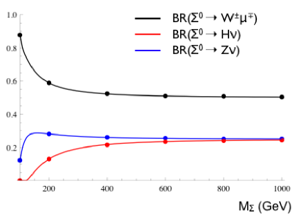
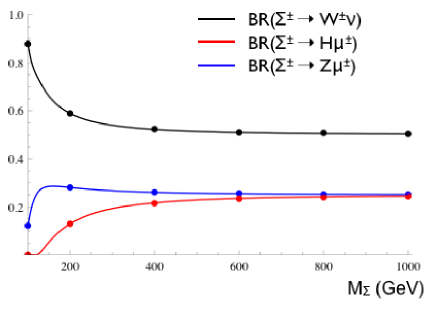
Figure 1: Branching ratios of the neutral component (left) and charged component (right) of the fermionic triplet in the case $V_{e}=V_{\tau}=0\,,\ V_{\mu}=0.063$. The dots correspond to numerically evaluated values while the lines correspond to the theoretical predictions. Notice that, as expected from Eqs. (90)-(95) in the case of one non-zero mixing angle, the result is the same for charged and neutral triplet decay.

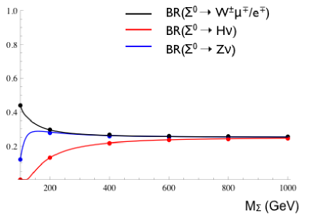
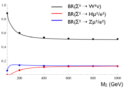
Figure 2: Branching ratios of the neutral component (left) and charged component (right) of the fermionic triplet in the case $V_{\tau}=0\,,\ V_{e}=V_{\mu}=4.1\cdot 10^{-4}$. The dots correspond to numerically evaluated values while the lines correspond to the theoretical predictions while the lines correspond to the theoretical predictions. When both channel with $e$ and $\mu$ are open, only one is displayed, since, for this particular choice of the mixing angles, they are overlapped.

As a second step of the validation procedure, we have computed the cross sections of a selection of $2\rightarrow 2$ processes that should not be influenced by the presence of triplets using MadGraph/MadEvent and we have compared the results obtained with typeIIIseesaw_MG and sm_FR. Results are gathered in Table 5 in Appendix B: an agreement at the level of $1\%$ is found.

Finally, we have checked that the production of a pair of triplets at the LHC with a center-of-mass energy of 14 TeV obtained with MadGraph/MadEvent matches the previous results in the literature [7, 8], see Table 6 in Appendix B.

4 The minimal type III seesaw model at the LHC at 7 TeV

4.1 Bounds on the mixing angles

In Refs. [10, 13, 14] the bounds on the parameters of the type III seesaw model have been derived. The bounds apply to the following combination of parameters:

$$\frac{v^{2}}{2}\left|Y^{\dagger}M^{-2}Y\right|_{\alpha\beta}=\left|V_{\alpha}V_{\beta}\right|.$$ (96)

We have then the following constraints:

$$|V_{e}| < 5.5\cdot 10^{-2}$$ (97)

$$|V_{\mu}| < 6.3\cdot 10^{-2}$$ (98)

$$|V_{\tau}| < 6.3\cdot 10^{-2}$$ (99)

$$|V_{e}V_{\mu}| < 1.7\cdot 10^{-7}$$ (100)

$$|V_{e}V_{\tau}| < 4.2\cdot 10^{-4}$$ (101)

$$|V_{\mu}V_{\tau}| < 4.9\cdot 10^{-4}.$$ (102)

Notice that if only $V_{e}$ or $V_{\mu}$ is present the stronger constrain of Eq. (100) does not apply and $\mathcal{O}(10^{-2})$ mixings are allowed. On the other side, if both are different from zero, then either one of the two is much smaller than the other, effectively reducing this case to the one with only one non-zero $V_{\alpha}$, or they are both $\mathcal{O}(10^{-3})$, in order to satisfy the strong bound of Eq. (100). However, as we will discuss later, since the production of the triplet happens via gauge interactions, reducing the mixing angle will not reduce the total cross section, so that these bounds have to be taken into account, but the mixing angles are not as crucial as in the type I seesaw.

In this paper we are going to focus on a specific case, in order to illustrate how our model works and to show that even with the LHC running at 7 TeV there is the possibility of testing the low scale type III seesaw. We are going to give the cross section of the relevant channels for the case $V_{e}=V_{\tau}=0\ ,\ V_{\mu}=0.063$. This case corresponds to the maximum allowed mixing angles. If the mixing is so large, then some cancellation or an extended seesaw mechanism like the inverse seesaw must be invoked in order to obtain the correct value for neutrino masses. However, all the discussion we perform in this section applies also in the case of small mixing. In the next sections we are going to discuss the triplet production and decays, give the cross sections which are relevant for discovery and discuss the main backgrounds which affect the measurement and the main cuts that could be implemented in order to reduce it. A more detailed study is beyond the scope of this work.

4.2 Triplet production and decay

At the LHC triplets are mainly produced in pair. In Table 2 production cross sections for different mass values are collected, with the acceptance cuts listed in Table 3. Since the triplets are produced via gauge interactions, the production cross sections do not depend on the mixing parameters. After production, the triplets decay inside the detector according to the expressions displayed in Eqs. (90)-(95). While the decay width depends strongly on the value of the mixing angles $V_{\alpha}$, the branching ratios dependence is very mild. Since we are always in the narrow width regime, the total cross section is driven only by the mass of the triplet (for the production) and its branching ratios (for the decays). Therefore, a non-discovery at the LHC will permit to constrain the mass of the triplet, after some assumption on the branching ratios have been done.

Once the triplets have decayed into leptons and gauge bosons, the latter will then decay into charged leptons, quarks, which will show up as jets (and leptons, when heavy quarks decay semileptonically), and neutrinos, which will manifest themselves as missing energy. Final states can be classified according to the number of charged leptons. The type III seesaw can give rise to final states with up to 6 leptons. However, it has been shown that the cross sections for 6-, 5- and 4-leptons final states is to low for being useful for discovery, already at 14 GeV [7]; therefore, we will not consider them here . On the other hand, the most promising channels are the 3-leptons and the dileptons, i.e. with 2 leptons of the same sign. In the following sections we are going to discuss these channels and the main backgrounds which affect them.

$M_{\Sigma}$	$\sigma(pp\to\Sigma^{+}\Sigma^{0})(fb)$	$\sigma(pp\to\Sigma^{+}\Sigma^{-})(fb)$	$\sigma(pp\to\Sigma^{-}\Sigma^{0})(fb)$
100	4.329e+3	3.339e+3	2.325e+3
120	2.157e+3	1.629e+3	1.106e+3
140	1.200e+3	8.882e+2	5.894e+2
160	7.215e+2	5.229e+3	3.387e+2
180	4.555e+2	3.249e+2	2.059e+2
200	3.006e+2	2.109e+2	1.311e+2
300	5.488e+1	3.580e+1	2.027e+1
400	1.434e+1	8.777	4.632
600	1.527	8.576e-1	4.118e-1
800	2.097e-1	1.132e-1	5.139e-2
1000	3.133e-2	1.774e-2	7.401e-2

Table 2: Production cross sections at 7 TeV.

Acceptance Cuts
$p_{T_{j}}>20\,\rm{GeV}$	$\eta_{j}<5$	$\Delta R_{jj}>0.001$
$p_{T_{\ell}}>10\,\rm{GeV}$	$\eta_{\ell}<2.5$	$\Delta R_{\ell\ell}>0$

Table 3: Acceptance cuts used for production simulations at 7 TeV and 14 TeV.

4.3 The most relevant final states

Tables 7 and 8 in Appendix C display the cross sections for the intermediate and final states with 2 and 3 leptons at different mass energies.  While the intermediate ones are calculated with MadGraph, the final ones are obtained by multiplication with the corresponding branching ratios. From a quick look to these tables one can see that even with LHC running at 7 TeV, with the few fb^-1 of luminosity which are expected to be reached by the end of 2011, several events are expected, for low triplet mass. In the 3-leptons table, in the total cross section we have isolated the channels with leptons not-coming from Z decay. Indeed, when the cut on the invariant mass of the leptons will be applied in order to reduce the background events coming from Z decay (see later), these events will mostly disappear. Then the numbers we quote in blue in Table 8 can be considered the effective cross section after the application of this cut.

By looking at these table we see that there are 4 possible final states with 2 and 3 leptons:

• 3 leptons + missing transverse energy (MET);

• 3 leptons + 2 jets + MET;

• 2 same-sign leptons + 4 jets;

• 2 same-sign leptons + 2 jets + MET.

In what follows we are going to discuss the main features of all of them. We have simulated $pp\rightarrow\Sigma^{+}\Sigma^{0}\rightarrow\mu^{+}\mu^{+}\mu^{-}+\nu s(+jets)$ with MadGraph/MadEvents, hadronization being obtained with the help of PYTHIA [15]. The CMS detector has been simulated via the PGS software [16].

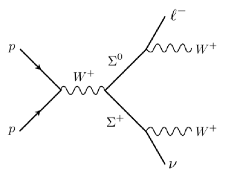
Figure 3: Dominant process for the discovery channel for the fermionic triplet at the LHC.

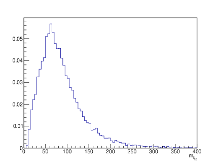
Figure 4: Invariant mass of the two $\mu^{+}$ for a luminosity of $30\rm{fb}^{-1}$ and $M_{\Sigma}=100~{}\rm{GeV}$. Pre-selection cuts selected only the events with 3 charged leptons among which 2 positive muons.

3 leptons + MET. This is probably the best discovery channel: indeed the background is more easily reduced due to the absence of jets in the final state. The dominant process generating it is depicted in Fig. 3. In an ideal detector where jets are not misidentified with leptons, the only background sources would be $WW$, $WWW$, $WZ$ and $ZZ$ when a lepton is missed. In practice jets should be added to these background; however, as it is discussed later, all these background should be under control.

In this channel, the invariant mass $m_{\mu^{+}\mu^{+}}$ of the two same-sign muons presents a long tail in the high energy region that is characteristic of the presence of new physics, see Fig. 4, and can be exploited to reduce the background. Moreover, this is typical of this kind of seesaw, permitting thus to distinguish among type I, II and III [7].

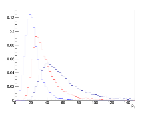
Figure 5: $p_{T}$ distribution of the different leptons for $M_{\Sigma}=100~{}\rm{GeV}$. The black, red and blue curves represent the lepton with the highest, intermediate and smallest $p_{T}$ respectively. Pre-selection cuts selected only the events with 3 charged leptons among which 2 positive muons.

3 leptons + 2 jets + MET. This channel is probably the best one in order to reconstruct the mass of the triplet. Moreover it can be used also to discriminate between type II and type III seesaw [7]. It also appears in the type I seesaw with a gauged $U(1)_{B-L}$ [17]. In this case the reduction of the background can be more complicated, due to the impossibility of applying a jet veto. Essentially all the sources listed in the next section constitute a background for this channel. A precise estimation of the sensitivity to this new physics would require the complete simulation of the background and a detailed analysis, which is beyond the scope of this work. However, we will show later that the possibility of reducing the background to “reasonable” levels is realistic.

Once the triplet has been observed, its mass needs to be measured. To this aim, this channel, emerging from the process $pp\rightarrow(\Sigma^{\pm}\rightarrow\ell^{\pm}Z/H)(\Sigma^{0}\rightarrow\ell^{\pm}W^{\mp})$ with $Z/H$ decaying into jets, is the best one. Indeed the momentum of the $Z/H$ boson is reconstructed from the jets momenta, while its combination with the momentum of one of the two same-sign leptons gives the mass of the charged triplet. Since there are two possibilities for this combination, the chosen one will be that giving closest invariant mass for the recontructed charged and neutral triplets, where the latter is given by the combination of the momenta of the two remaining leptons $plus$ MET .

The reconstructed mass of the charged and neutral triplet are shown in Fig. 6 where no cuts has been applied. Note that a selection cut on the invariant mass $m_{jj}$ of the jets

$$|m_{jj}-M_{Z/H}|<10\,\rm{GeV}$$ (103)

will improve the mass reconstruction.

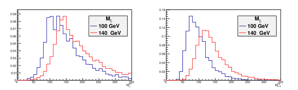
Figure 6: Reconstructed mass of the charged triplet (left) and neutral triplet (right), for a luminosity of $30\rm{fb}^{-1}$, in the case $M_{\Sigma}=100~{}\rm{GeV}$ (black curve) and $M_{\Sigma}=140~{}\rm{GeV}$ (red curve). Pre-selection cuts selected only the events with 3 charged leptons and at least 2 jets.

Even if the background is added, a clear peak in the reconstructed mass will still be visible, which should also permit to distinguish from type II seesaw [7].

2 same-sign leptons + jets (+MET) As it is clear from Table 7, the cross section for these final states are quite large, even larger than the ones for 3 leptons final states. However here jets are always present, which can render a bit more difficult the background reduction. The backgrounds are essentially the same as in the previous channel and indeed it has been shown [7] that the discovery and the discriminatory potentials of the 2- and 3-leptons final states are similar too. A realistic study, especially a study on real data, should consider this channel as well.

4.4 Background

The main background sources for the channels discussed above are : $t\overline{t}$, $t\overline{t}W$, $WW$, $WZ$, $ZZ$, $Zt\overline{t}$, $Zb\overline{b}$ and 3 gauge bosons. The same background plus additional jets should be considered as well, both if looking at final states with jets or no: some jets can be indeed misidentified as leptons. In the following we will give a brief description of each background and of the cuts that can be implemented in order to reduce it. Whenever the cross section for the different background under study has not been measured, we have used MadGraph/MadEvent to obtain the cross-sections for LHC running at 7 TeV and compared our results with previous results obtained by the CMS collaboration [18] whenever possible. All backgrounds have been simulated with 0 and 1 additional jets.

$\mathbf{t\overline{t}.}$ The production of a pair of top quarks decaying into $bW$, one of the $b$ giving a lepton and the W decaying leptonically, is a source of background with a large cross section. At 7 TeV the production of a top quarks pair has been measuread by CMS [19] and ATLAS [20] to be $\sigma_{t\overline{t}}=(173^{+39}_{-32})\,\rm{pb}$ and $(171\pm 20\pm 14^{+8}_{-6})\,\rm{pb}$, with an integrated luminosity of 36 and 35 pb^-1, respectively. Combining the branching ratio $BR(W\rightarrow l\nu)=30\%$ with the $10\%$ of branching ratio for the semileptonic decay of the $b$, the final cross section for such background should be around $0.15-1.5\,\rm{pb}$ depending on how many different lepton flavors one expect in the final state. In the case where the signal final state does not contain jets (at the parton level), a cut on the number of jets will reduce this background to negligible levels. $b$-tagging could be applied in order to reduce it when channels with jets are considered.

$\mathbf{t\overline{t}W.}$ Here the two tops decay into a $W$ plus jets. The third $W$ ensures the presence of three leptons in the final state. The presence of jets makes this background negligible when looking to three leptons + MET without jets. On the other hand, when channels with jets are considered, this background should be carefully studied. We found $\sigma_{ttWj}\sim 230~{}\rm{fb}$. The production cross section for $t\bar{t}W$ should then be larger, but considering the appropriate branching fractions, the final cross sections should be of few fb, depending on the number of jets.

$\mathbf{WW.}$ This is a large source of background. At $7$ TeV, it has been measured by CMS [21] and ATLAS [22] to be : $\sigma_{WW}=41.1\pm 15.3\rm{(stat.)}\pm 5.8\rm{(syst.)}\pm 4.5\rm{(lumi.)}~{}\rm{pb}$ and $\sigma_{WW}=41^{+20}_{-16}\rm{(stat.)}\pm 5\rm{(syst.)}\pm 1\rm{(lumi.)}~{}\rm{pb}$, with an integrated luminosity of 36 and 34 pb^-1, respectively. CMS collaboration also found [23] : $\sigma(pp\rightarrow WW+X)=55.3\pm 3.3\rm{(stat.)}\pm 6.9\rm{(syst.)}\pm 3.3\rm{(lumi.)}~{}pb$. But pre-selection cuts (3 charged leptons out of which 2 have the same sign, 2 hard leptons) should reduce it to a negligible level.

$\mathbf{WZ.}$ The CMS collaboration measured [23] : $\sigma(pp\rightarrow WZ+X)=17.0\pm 2.4\rm{(stat.)}\pm 1.1\rm{(syst.)}\pm 1.0\rm{(lumi.)}~{}pb$. This will give $\sim 60$ fb for the final state cross section. A cut on the invariant mass of two leptons with opposite sign, $|M_{Z}-m_{ll}|>10~{}\rm{GeV}$ , can be applied in order to eliminate leptons coming from $Z$ decay. Moreover, if one considers leptons with different flavour, like for instance the channel $e^{-}\mu^{+}\mu^{+}$ + MET, this will be free from such a background.

$\mathbf{ZZ.}$ This channel is a background when one of the lepton is lost. It has been measured at the LHC by the CMS collaboration [23] : $\sigma(pp\rightarrow ZZ+X)=3.8^{+1.5}_{-1.2}\rm{(stat.)}\pm 0.2\rm{(syst.)}\pm 0.2\rm{(lumi.)}~{}pb$. Again, cuts on the invariant mass of opposite signs leptons should allow to reduce it to a negligible level.

$\mathbf{t\overline{t}Z}$ and $\mathbf{b\overline{b}Z.}$ These constitute a background for final states involving jets. The production cross section is relatively large: $\sigma_{t\overline{t}Z}=205~{}\rm{fb}$ and $\sigma_{b\overline{b}Z}=50~{}\rm{pb}$. However, the cuts on the invariant mass of the leptons as well as $b$-tagging should reduce them to negligible levels.

$\mathbf{WWW.}$ Among the 3 gauge bosons background, this is the one with highest cross section. The production cross-section for three $W$ bosons is anyway lower than other background considered: $\sigma_{WWW}=71~{}\rm{fb}$, which becomes really negligible when the final state is considered.

All theses background sources can be reduces by cuts on the $p_{T}$ of the leptons which are hard in the signal final state. Additional cuts on number of jets or opposite-sign leptons’ invariance mass can further help to improve the signal over background ratio.

As it is clear, the aim of this section was just to describe the main backgrounds affecting the considered signals. In order to give precise estimation the entire simulation of the background should be performed.

4.5 Other relevant cases

Even if we have discussed in details only the case of large mixing with muons, there are other cases which can be relevant. Here we briefly sketch their characteristics.

Mixing with electrons or taus.

As already discussed in the literature [7], the situation for mixing with electrons is similar to the one with muons and our analisis can be applied to it as well. On the other side, since detecting taus is more complicated, the discovery potential of channels involving taus is believed to be smaller.

Mixing with 2 or 3 charged leptons.

In such a case the triplet can couple to more than one family. The mixing angles are thus more constrained. As we have already shown (see Figs. 1-2), the simultaneous presence of two (or three) non zero $V_{\alpha}$ would reduce the corresponding branching ratio by a small factor: if, for instance, two of them are taken to be equal, then the corresponding branching ratio will be decreased by a factor 2 with respect to the case with only one non-zero mixing angle (see Figs. 1-2). However the pair production cross section of triplets is not affected by the mixing values and thus only the branching ratios and the mass of the triplet drive the relevant processes studied here.

Small mixing angles, $\boldsymbol{\mathcal{O}(10^{-6})}$.

This case is the “most natural” one, since here small neutrino masses can be accomodated without any cancellation or further source of suppression . Such small mixing angles drastically reduce the value of the triplet decay width, so that displaced vertexes up to few millimeters can be present (see also [8]). In case of finding an excess of events in some of the considered channels, the measurement of these displaced vertexes could be a clear signal that we are in presence of this kind of physics. The possible presence of a displaced vertex have to be taken into account when defining the reconstruction parameters for the data analisis (for example to reconstruct an interaction vertex). A detailed study of this topic is postponed to the analisis of real data. A part from this, in general the cross sections are not affected and the analisis can proceed as in the case of large mixing.

5 Conclusions

In this paper we have described in details the minimal type III seesaw model and its implementation in FeynRules/MadGraph. In particular we have explicitly written all the couplings and we have discussed the tests we have performed in order to validate the implemented model. Even if the model has been tested only with MadGraph which uses the unitary gauge, the Goldstone bosons have been implemented as well, so that it can be used also with other Monte Carlo generators such as CalcHep [24]. As already stressed in the Introduction, this is a necessary step to be done before proceeding to the analysis of real LHC data.

In order to show an example of the utility of our model, we have focused on a particular case –large mixing with muons, $V_{\mu}=0.063$, and small triplet masses, 100 GeV, 120 GeV, 140 GeV– and for these cases we have calculated the cross sections of the relevant channels at the LHC running at 7 TeV. We have shown that several events are expected for a luminosity of few fb^-1. We have discussed the main background sources and the methods that can be employed in order to reduce it. A more detailed study is beyond the scope of this work, but, still at this level, we can expect that a discovery at the LHC is possible, even in the 2011 run, if the mass of the triplet is low enough and the background rejection is good. Otherwise, in case of non-discovery, an upgrade of the bounds on the triplet mass can be set.

Appendix A The explicit Lagrangian in the minimal model

$${\color[rgb]{0,0,1}g^{CC}_{L}} = \left(\begin{array}[]{cc}\left(1+\frac{V^{T}\wedge V}{2}\right)\mathcal{U}_{PMNS}&-V^{T}\\ 0&\sqrt{2}\left(1-\frac{V\cdot V^{T}}{2}\right)\end{array}\right)\ =\$$ (106)

$$=\left(\begin{array}[]{ccc}(\mathcal{U}_{PMNS})_{e1}+\frac{V_{e}V_{\alpha}}{2}(\mathcal{U}_{PMNS})_{\alpha 1}&(\mathcal{U}_{PMNS})_{e2}+\frac{V_{e}V_{\alpha}}{2}(\mathcal{U}_{PMNS})_{\alpha 2}&(\mathcal{U}_{PMNS})_{e3}+\frac{V_{e}V_{\alpha}}{2}(\mathcal{U}_{PMNS})_{\alpha 3}\\ (\mathcal{U}_{PMNS})_{\mu 1}+\frac{V_{\mu}V_{\alpha}}{2}(\mathcal{U}_{PMNS})_{\alpha 1}&(\mathcal{U}_{PMNS})_{\mu 2}+\frac{V_{\mu}V_{\alpha}}{2}(\mathcal{U}_{PMNS})_{\alpha 2}&(\mathcal{U}_{PMNS})_{\mu 3}+\frac{V_{\mu}V_{\alpha}}{2}(\mathcal{U}_{PMNS})_{\alpha 3}\\ (\mathcal{U}_{PMNS})_{\tau 1}+\frac{V_{\tau}V_{\alpha}}{2}(\mathcal{U}_{PMNS})_{\alpha 1}&(\mathcal{U}_{PMNS})_{\tau 2}+\frac{V_{\tau}V_{\alpha}}{2}(\mathcal{U}_{PMNS})_{\alpha 2}&(\mathcal{U}_{PMNS})_{\tau 3}+\frac{V_{\tau}V_{\alpha}}{2}(\mathcal{U}_{PMNS})_{\alpha 3}\\ 0&0&0\end{array}\right|$$ (111)

$$\left|\begin{array}[]{c}-V_{e}\\ -V_{\mu}\\ -V_{\tau}\\ \sqrt{2}(1-\frac{V_{e}^{2}+V_{\mu}^{2}+V_{\tau}^{2}}{2})\end{array}\right)$$ (116)

$${\color[rgb]{0,0,1}g^{CC}_{R}} = \left(\begin{array}[]{cc}0&-\sqrt{2}m_{l}V^{T}M_{\Sigma}^{-1}\\ -V\,\mathcal{U}_{PMNS}&1-\frac{V\cdot V^{T}}{2}\end{array}\right)=$$ (119)

$$=\left(\begin{array}[]{cccc}0&0&0&-\sqrt{2}M_{\Sigma}^{-1}m_{e}V_{e}\\ 0&0&0&-\sqrt{2}M_{\Sigma}^{-1}m_{\mu}V_{\mu}\\ 0&0&0&-\sqrt{2}M_{\Sigma}^{-1}m_{\tau}V_{\tau}\\ -V_{\alpha}(\mathcal{U}_{PMNS})_{\alpha 1}&-V_{\alpha}(\mathcal{U}_{PMNS})_{\alpha 2}&-V_{\alpha}(\mathcal{U}_{PMNS})_{\alpha 3}&1-\frac{V_{e}^{2}+V_{\mu}^{2}+V_{\tau}^{2}}{2}\end{array}\right)$$ (124)

$${\color[rgb]{0,0,1}g^{NC}_{L}} = \left(\begin{array}[]{cc}\frac{1}{2}-cos^{2}\theta_{W}-V^{T}\wedge V&\frac{1}{\sqrt{2}}V^{T}\\ \frac{1}{\sqrt{2}}V&V\cdot V^{T}-cos^{2}\theta_{W}\end{array}\right)=$$ (127)

$$=\left(\begin{array}[]{cccc}\frac{1}{2}-cos^{2}\theta_{W}-V_{e}^{2}&V_{e}V_{\mu}&V_{e}V_{\tau}&\frac{V_{e}}{\sqrt{2}}\\ V_{e}V_{\mu}&\frac{1}{2}-cos^{2}\theta_{W}-V_{\mu}^{2}&V_{\mu}V_{\tau}&\frac{V_{\mu}}{\sqrt{2}}\\ V_{e}V_{\tau}&V_{\mu}V_{\tau}&\frac{1}{2}-cos^{2}\theta_{W}-V_{\tau}^{2}&\frac{V_{\tau}}{\sqrt{2}}\\ \frac{V_{e}}{\sqrt{2}}&\frac{V_{\mu}}{\sqrt{2}}&\frac{V_{\tau}}{\sqrt{2}}&V_{e}^{2}+V_{\mu}^{2}+V_{\tau}^{2}-cos^{2}\theta_{W}\end{array}\right)$$ (132)

$${\color[rgb]{0,0,1}g^{NC}_{R}} = \left(\begin{array}[]{cc}1-cos^{2}\theta_{W}&\sqrt{2}m_{l}V^{T}M_{\Sigma}^{-1}\\ \sqrt{2}M_{\Sigma}^{-1}Vm_{l}&-cos^{2}\theta_{W}\end{array}\right)=$$ (135)

$$=\left(\begin{array}[]{cccc}1-cos^{2}\theta_{W}&0&0&\sqrt{2}M_{\Sigma}^{-1}m_{e}V_{e}\\ 0&1-cos^{2}\theta_{W}&0&\sqrt{2}M_{\Sigma}^{-1}m_{\mu}V_{\mu}\\ 0&0&1-cos^{2}\theta_{W}&\sqrt{2}M_{\Sigma}^{-1}m_{\tau}V_{\tau}\\ \sqrt{2}M_{\Sigma}^{-1}m_{e}V_{e}&\sqrt{2}M_{\Sigma}^{-1}m_{\mu}V_{\mu}&\sqrt{2}M_{\Sigma}^{-1}m_{\tau}V_{\tau}&-cos^{2}\theta_{W}\end{array}\right)$$ (140)

$${\color[rgb]{0,0,1}g^{NC}_{\nu}} = \left(\begin{array}[]{cc}1-\mathcal{U}_{PMNS}^{T}\,V^{T}\wedge V\,\mathcal{U}_{PMNS}&\mathcal{U}_{PMNS}^{T}V^{T}\\ V\,\mathcal{U}_{PMNS}&V\cdot V^{T}\end{array}\right)=$$ (143)

$$=\left(\begin{array}[]{cc}1-(\mathcal{U}_{PMNS})_{\alpha 1}V_{\alpha}V_{\beta}(\mathcal{U}_{PMNS})_{\beta 1}&-(\mathcal{U}_{PMNS})_{\alpha 1}V_{\alpha}V_{\beta}(\mathcal{U}_{PMNS})_{\beta 2}\\ -(\mathcal{U}_{PMNS})_{\alpha 2}V_{\alpha}V_{\beta}(\mathcal{U}_{PMNS})_{\beta 1}&1-(\mathcal{U}_{PMNS})_{\alpha 2}V_{\alpha}V_{\beta}(\mathcal{U}_{PMNS})_{\beta 2}\\ -(\mathcal{U}_{PMNS})_{\alpha 3}V_{\alpha}V_{\beta}(\mathcal{U}_{PMNS})_{\beta 1}&-(\mathcal{U}_{PMNS})_{\alpha 3}V_{\alpha}V_{\beta}(\mathcal{U}_{PMNS})_{\beta 2}\\ V_{\alpha}(\mathcal{U}_{PMNS})_{\alpha 1}&V_{\alpha}(\mathcal{U}_{PMNS})_{\alpha 2}\\ \end{array}\right|$$ (148)

$$\left|\begin{array}[]{cc}-(\mathcal{U}_{PMNS})_{\alpha 1}V_{\alpha}V_{\beta}(\mathcal{U}_{PMNS})_{\beta 3}&V_{\alpha}(\mathcal{U}_{PMNS})_{\alpha 1}\\ -(\mathcal{U}_{PMNS})_{\alpha 2}V_{\alpha}V_{\beta}(\mathcal{U}_{PMNS})_{\beta 3}&V_{\alpha}(\mathcal{U}_{PMNS})_{\alpha 2}\\ 1-(\mathcal{U}_{PMNS})_{\alpha 3}V_{\alpha}V_{\beta}(\mathcal{U}_{PMNS})_{\beta 3}&V_{\alpha}(\mathcal{U}_{PMNS})_{\alpha 3}\\ V_{\alpha}(\mathcal{U}_{PMNS})_{\alpha 3}&V_{e}^{2}+V_{\mu}^{2}+V_{\tau}^{2}\end{array}\right)$$ (153)

$${\color[rgb]{0,0,1}g^{H\ell}_{L}} = \left(\begin{array}[]{cc}\frac{m_{l}}{v}\left(1-3V^{T}\wedge V\right)&\sqrt{2}\frac{m_{l}}{v}V^{T}\\ \sqrt{2}\frac{M_{\Sigma}}{v}V\cdot(1-V^{T}\wedge V)+\sqrt{2}M_{\Sigma}^{-1}V\frac{m_{l}^{2}}{v}&2\frac{M_{\Sigma}}{v}V\cdot V^{T}\end{array}\right)=$$ (156)

$$=\left(\begin{array}[]{cc}\frac{m_{e}}{v}(1-3V_{e}^{2})&-3\frac{m_{e}}{v}V_{e}V_{\mu}\\ -3\frac{m_{\mu}}{v}V_{\mu}V_{e}&\frac{m_{\mu}}{v}(1-3V_{\mu}^{2})\\ -3\frac{m_{\tau}}{v}V_{\tau}V_{e}&-3\frac{m_{\tau}}{v}V_{\tau}V_{\mu}\\ \sqrt{2}\frac{M_{\Sigma}}{v}V_{e}(1-V_{e}^{2}-V_{\mu}^{2}-V_{\tau}^{2})+\sqrt{2}M_{\Sigma}^{-1}\frac{m_{e}^{2}}{v}V_{e}&\sqrt{2}\frac{M_{\Sigma}}{v}V_{\mu}(1-V_{e}^{2}-V_{\mu}^{2}-V_{\tau}^{2})+\sqrt{2}M_{\Sigma}^{-1}\frac{m_{\mu}^{2}}{v}V_{\mu}\end{array}\right|$$ (161)

$$\left|\begin{array}[]{cc}-3\frac{m_{e}}{v}V_{e}V_{\tau}&\sqrt{2}\frac{m_{e}}{v}V_{e}\\ -3\frac{m_{\mu}}{v}V_{\mu}V_{\tau}&\sqrt{2}\frac{m_{\mu}}{v}V_{\mu}\\ \frac{m_{\tau}}{v}(1-3V_{\tau}^{2})&\sqrt{2}\frac{m_{\tau}}{v}V_{\tau}\\ \sqrt{2}\frac{M_{\Sigma}}{v}V_{\tau}(1-V_{e}^{2}-V_{\mu}^{2}-V_{\tau}^{2})+\sqrt{2}M_{\Sigma}^{-1}\frac{m_{\tau}^{2}}{v}V_{\tau}&2\frac{M_{\Sigma}}{v}(V_{e}^{2}+V_{\mu}^{2}+V_{\tau}^{2})\end{array}\right)$$ (166)

$${\color[rgb]{0,0,1}g^{H\nu}_{L}} = \left(\begin{array}[]{cc}\frac{\sqrt{2}}{v}m_{\nu}^{d}&\frac{\sqrt{2}}{v}m_{\nu}^{d}\mathcal{U}_{PMNS}^{T}V^{T}\\ \frac{\sqrt{2}}{v}\left(1-\epsilon^{\prime}\right)M_{\Sigma}V\mathcal{U}_{PMNS}&\frac{\sqrt{2}}{v}M_{\Sigma}\epsilon^{\prime}\end{array}\right)=$$ (169)

$$=\frac{\sqrt{2}}{v}\left(\begin{array}[]{cccc}m_{\nu 1}&0&0&m_{\nu 1}{\mathcal{U}_{PMNS}}_{\alpha 1}V_{\alpha}\\ 0&m_{\nu 2}&0&m_{\nu 2}{\mathcal{U}_{PMNS}}_{\alpha 2}V_{\alpha}\\ 0&0&m_{\nu 3}&m_{\nu 3}{\mathcal{U}_{PMNS}}_{\alpha 3}V_{\alpha}\\ \left(1-\epsilon^{\prime}\right)M_{\Sigma}V_{\alpha}{\mathcal{U}_{PMNS}}_{\alpha 1}&\left(1-\epsilon^{\prime}\right)M_{\Sigma}V_{\alpha}{\mathcal{U}_{PMNS}}_{\alpha 2}&\left(1-\epsilon^{\prime}\right)M_{\Sigma}V_{\alpha}{\mathcal{U}_{PMNS}}_{\alpha 3}&M_{\Sigma}\epsilon^{\prime}\end{array}\right)$$ (174)

$${\color[rgb]{0,0,1}g^{\eta\ell}_{L}} = \left(\begin{array}[]{cc}-\frac{m_{l}}{v}(1+V^{T}\wedge V)&-\frac{m_{l}}{v}\sqrt{2}V^{T}\\ \frac{M_{\Sigma}}{v}\sqrt{2}V(1-V^{T}\wedge V-\frac{m^{2}_{l}}{M_{\Sigma}^{2}})&\frac{2M_{\Sigma}}{v}V\cdot V^{T}\end{array}\right)=$$ (177)

$$=\left(\begin{array}[]{cc}-\frac{m_{e}}{v}(1+V_{e}^{2})&-\frac{m_{e}}{v}V_{e}V_{\mu}\\ -\frac{m_{\mu}}{v}V_{\mu}V_{e}&-\frac{m_{\mu}}{v}(1+V_{\mu}^{2})\\ -\frac{m_{\tau}}{v}V_{\tau}V_{e}&-\frac{m_{\tau}}{v}V_{\tau}V_{\mu}\\ \sqrt{2}\frac{M_{\Sigma}}{v}V_{e}(1-V_{e}^{2}-V_{\mu}^{2}-V_{\tau}^{2})-\sqrt{2}M_{\Sigma}^{-1}\frac{m_{e}^{2}}{v}V_{e}&\sqrt{2}\frac{M_{\Sigma}}{v}V_{\mu}(1-V_{e}^{2}-V_{\mu}^{2}-V_{\tau}^{2})-\sqrt{2}M_{\Sigma}^{-1}\frac{m_{\mu}^{2}}{v}V_{\mu}\end{array}\right|$$ (182)

$$\left|\begin{array}[]{cc}-\frac{m_{e}}{v}V_{e}V_{\tau}&-\sqrt{2}\frac{m_{e}}{v}V_{e}\\ -\frac{m_{\mu}}{v}V_{\mu}V_{\tau}&-\sqrt{2}\frac{m_{\mu}}{v}V_{\mu}\\ -\frac{m_{\tau}}{v}(1+V_{\tau}^{2})&-\sqrt{2}\frac{m_{\tau}}{v}V_{\tau}\\ \sqrt{2}\frac{M_{\Sigma}}{v}V_{\tau}(1-V_{e}^{2}-V_{\mu}^{2}-V_{\tau}^{2})-\sqrt{2}M_{\Sigma}^{-1}\frac{m_{\tau}^{2}}{v}V_{\tau}&2\frac{M_{\Sigma}}{v}(V_{e}^{2}+V_{\mu}^{2}+V_{\tau}^{2})\end{array}\right)$$ (187)

$${\color[rgb]{0,0,1}g_{L}^{\phi}}=\left(\begin{array}[]{cc}\sqrt{2}\frac{m_{l}}{v}(1-\frac{V^{T}\wedge V}{2})\mathcal{U}_{PMNS}&\frac{\sqrt{2}}{v}m_{l}V^{T}\\ 2M_{\Sigma}^{-1}V\frac{m_{l}^{2}}{v}\mathcal{U}_{PMNS}&0\end{array}\right)=$$ (190)

$$=\left(\begin{array}[]{cccc}\frac{\sqrt{2}}{v}(m_{e}(\delta_{e\alpha}-\frac{V_{e}V_{\alpha}}{2})\mathcal{U}_{PMNS_{\alpha 1}})&\frac{\sqrt{2}}{v}(m_{e}(\delta_{e\alpha}-\frac{V_{e}V_{\alpha}}{2})\mathcal{U}_{PMNS_{\alpha 2}})&\frac{\sqrt{2}}{v}(m_{e}(\delta_{e\alpha}-\frac{V_{e}V_{\alpha}}{2})\mathcal{U}_{PMNS_{\alpha 3}})&\frac{\sqrt{2}}{v}m_{e}V_{e}\\ \frac{\sqrt{2}}{v}(m_{\mu}(\delta_{\mu\alpha}-\frac{V_{\mu}V_{\alpha}}{2})\mathcal{U}_{PMNS_{\alpha 1}})&\frac{\sqrt{2}}{v}(m_{\mu}(\delta_{\mu\alpha}-\frac{V_{\mu}V_{\alpha}}{2})\mathcal{U}_{PMNS_{\alpha 2}})&\frac{\sqrt{2}}{v}(m_{\mu}(\delta_{\mu\alpha}-\frac{V_{\mu}V_{\alpha}}{2})\mathcal{U}_{PMNS_{\alpha 3}})&\frac{\sqrt{2}}{v}m_{\mu}V_{\mu}\\ \frac{\sqrt{2}}{v}(m_{\tau}(\delta_{\tau\alpha}-\frac{V_{\tau}V_{\alpha}}{2})\mathcal{U}_{PMNS_{\alpha 1}})&\frac{\sqrt{2}}{v}(m_{\tau}(\delta_{\tau\alpha}-\frac{V_{\tau}V_{\alpha}}{2})\mathcal{U}_{PMNS_{\alpha 2}})&\frac{\sqrt{2}}{v}(m_{\tau}(\delta_{\tau\alpha}-\frac{V_{\tau}V_{\alpha}}{2})\mathcal{U}_{PMNS_{\alpha 3}})&\frac{\sqrt{2}}{v}m_{\tau}V_{\tau}\\ 2M^{-1}_{\Sigma}V_{\alpha}\frac{m_{\alpha}^{2}}{v}\mathcal{U}_{PMNS_{\alpha 1}}&2M^{-1}_{\Sigma}V_{\alpha}\frac{m_{\alpha}^{2}}{v}\mathcal{U}_{PMNS_{\alpha 2}}&2M^{-1}_{\Sigma}V_{\alpha}\frac{m_{\alpha}^{2}}{v}\mathcal{U}_{PMNS_{\alpha 3}}&0\end{array}\right)$$ (195)

$${\color[rgb]{0,0,1}g_{R}^{\phi}}=\left(\begin{array}[]{cc}-\sqrt{2}\mathcal{U}_{PMNS}\frac{m_{\nu}^{d}}{v}&(V^{T}-(V^{T}\wedge V)\cdot V^{T}-V^{T}\cdot\frac{V.V^{T}}{2})\sqrt{2}\frac{M_{\Sigma}}{v}-2\sqrt{2}\mathcal{U}_{PMNS}\frac{m_{\nu}^{d}}{v}\mathcal{U}_{PMNS}^{T}V^{T}\\ -2\frac{M_{\Sigma}}{v}V(1-\frac{(V^{T}\wedge V)}{2})\mathcal{U}_{PMNS}&0\end{array}\right)=$$ (198)

$$=\left(\begin{array}[]{cccc}-\frac{\sqrt{2}}{v}m_{\nu_{1}}\mathcal{U}_{e1}&-\frac{\sqrt{2}}{v}m_{\nu_{2}}\mathcal{U}_{e2}&-\frac{\sqrt{2}}{v}m_{\nu_{3}}\mathcal{U}_{e3}\\ -\frac{\sqrt{2}}{v}m_{\nu_{1}}\mathcal{U}_{\mu 1}&-\frac{\sqrt{2}}{v}m_{\nu_{2}}\mathcal{U}_{\mu 2}&-\frac{\sqrt{2}}{v}m_{\nu_{3}}\mathcal{U}_{\mu 3}\\ -\frac{\sqrt{2}}{v}m_{\nu_{1}}\mathcal{U}_{\tau 1}&-\frac{\sqrt{2}}{v}m_{\nu_{2}}\mathcal{U}_{\tau 2}&-\frac{\sqrt{2}}{v}m_{\nu_{3}}\mathcal{U}_{\tau 3}\\ \frac{M_{\Sigma}}{v}V_{\alpha}(V_{e}^{2}+V_{\mu}^{2}+V_{\tau}^{2}-2)\mathcal{U}_{\alpha 1}&\frac{M_{\Sigma}}{v}V_{\alpha}(V_{e}^{2}+V_{\mu}^{2}+V_{\tau}^{2}-2)\mathcal{U}_{\alpha 2}&\frac{M_{\Sigma}}{v}V_{\alpha}(V_{e}^{2}+V_{\mu}^{2}+V_{\tau}^{2}-2)\mathcal{U}_{\alpha 3}\end{array}\right|$$ (203)

$$\left|\begin{array}[]{c}\sqrt{2}\frac{M_{\Sigma}}{v}V_{e}(1-\frac{3}{2}(V_{e}^{2}+V_{\mu}^{2}+V_{\tau}^{2}))-2\sqrt{2}\frac{m_{\nu_{i}}}{v}\mathcal{U}_{ei}\mathcal{U}_{\alpha i}V_{\alpha}\\ \sqrt{2}\frac{M_{\Sigma}}{v}V_{\mu}(1-\frac{3}{2}(V_{e}^{2}+V_{\mu}^{2}+V_{\tau}^{2}))-2\sqrt{2}\frac{m_{\nu_{i}}}{v}\mathcal{U}_{\mu i}\mathcal{U}_{\alpha i}V_{\alpha}\\ \sqrt{2}\frac{M_{\Sigma}}{v}V_{\tau}(1-\frac{3}{2}(V_{e}^{2}+V_{\mu}^{2}+V_{\tau}^{2}))-2\sqrt{2}\frac{m_{\nu_{i}}}{v}\mathcal{U}_{\tau i}\mathcal{U}_{\alpha i}V_{\alpha}\\ 0\end{array}\right)$$ (208)

In the above expressions repetead flavour indexes are summed. As we will discuss later, we will take neutrino masses equal to zero, except in the case of small mixing angles .

Appendix B Tables for the validation of the implementation

Process	sm_FR	typeIIIseesaw1_MG	comparison
top decay	1.53174916	1.55409729	1.45899%
W decay	2.00335798	2.00322925	0.00642571%
Z decay	2.41539342	2.41481975	0.0237506%
BR(w+ $\to$ v e+ )	1.11025062e-01	1.11142e-01	0.105326%
BR(w+ $\to$ v m+ )	1.11036355e-01	1.11331e-01	0.265359%
BR(w+ $\to$ v tt+ )	1.12013868e-01	1.11018e-01	0.8962%
BR(w+ $\to$ c d  )	1.69615944e-02	1.69574065e-02	0.0246905%
BR(w+ $\to$ u d  )	3.14853587e-01	3.16304871e-01	0.460939%
BR(w+ $\to$ c s  )	3.17238100e-01	3.16278512e-01	0.302482%
BR(w+ $\to$ u s  )	1.68714343e-02	1.69683505e-02	0.574441%
BR(z $\to$ e- e+ )	3.45878542e-02	3.45049797e-02	0.239606%
BR(z $\to$ m- m+ )	3.46182266e-02	3.49703234e-02	1.01709%
BR(z $\to$ tt- tt+ )	3.45433552e-02	3.45770661e-02	0.0975901%
BR(z $\to$ invisible)	0.205237	0.205557	0.155917%
BR(z $\to$ b b  )	1.51238258e-01	1.50200176e-01	0.686388%
BR(z $\to$ c c  )	1.17361782e-01	1.17167722e-01	0.165352%
BR(z $\to$ d d  )	1.52782011e-01	1.52925551e-01	0.0939509%
BR(z $\to$ s s  )	1.52615959e-01	1.51787006e-01	0.543163%
BR(z $\to$ u u  )	1.17015696e-01	1.18309630e-01	0.10578%

Table 4: Comparison of decay widths and branching ratios between the model sm_FR and typeIIIseesaw1_MG.

Process	sm_FR	typeIIIseesaw1_MG	comparison
$e^{+}e^{-}\rightarrow e^{+}e^{-}$	$7.457\rm{e}{+2}$	$7.450\rm{e}{+2}$	0.095 %
$e^{+}e^{-}\rightarrow\mu^{+}\mu^{-}$	$1.125\rm{e}{-1}$	$1.126\rm{e}{-1}$	0.09 %
$e^{+}e^{-}\rightarrow\nu^{+}\nu^{-}$	$5.185\rm{e}{+1}$	$5.180\rm{e}{+1}$	0.10%
$\tau^{+}\tau^{-}\rightarrow W^{+}W^{-}$	$2.629\rm{e}{+0}$	$2.625\rm{e}{+0}$	0.15%
$\tau^{+}\tau^{-}\rightarrow ZZ$	$1.448\rm{e}{-1}$	$1.449\rm{e}{-1}$	0.07%
$\tau^{+}\tau^{-}\rightarrow Z\gamma$	$7.208\rm{e}{-1}$	$7.219\rm{e}{-1}$	0.15%
$\tau^{+}\tau^{-}\rightarrow\gamma\gamma$	$1.020\rm{e}{+0}$	$1.020\rm{e}{+0}$	–
$ZZ\rightarrow ZZ$	$5.997\rm{e}{-1}$	$5.996\rm{e}{-1}$	0.017%
$W^{+}W^{-}\rightarrow ZZ$	$2.996\rm{e}{+2}$	$2.995\rm{e}{+2}$	0.033%
$HH\rightarrow ZZ$	$6.763\rm{e}{+1}$	$6.763\rm{e}{+1}$	–
$HH\rightarrow W^{+}W^{-}$	$1.046\rm{e}{+2}$	$1.039\rm{e}{+2}$	0.57%
$GG\rightarrow GG$	$3.084\rm{e}{+5}$	$3.079\rm{e}{+5}$	0.16%
$u\overline{u}\rightarrow GG$	$1.981\rm{e}{+2}$	$1.980\rm{e}{+2}$	0.05%
$u\overline{u}\rightarrow W^{+}W^{-}$	$8.711\rm{e}{-1}$	$8.720\rm{e}{-1}$	0.10%
$u\overline{u}\rightarrow ZZ$	$8.783\rm{e}{-2}$	$8.800\rm{e}{-2}$	0.19%
$u\overline{u}\rightarrow Z\gamma$	$1.215\rm{e}{-1}$	$1.216\rm{e}{-1}$	0.08%
$u\overline{u}\rightarrow\gamma\gamma$	$6.725\rm{e}{-2}$	$6.714\rm{e}{-2}$	0.13%
$u\overline{u}\rightarrow s\overline{s}$	$7.809\rm{e}{+0}$	$7.807\rm{e}{+0}$	0.026 %
$u\overline{d}\rightarrow c\overline{s}$	$1.040\rm{e}{-1}$	$1.040\rm{e}{-1}$	–
$u\overline{s}\rightarrow c\overline{d}$	$3.000\rm{e}{-4}$	$2.999\rm{e}{-4}$	0.033%
$t\overline{t}\rightarrow GG$	$7.352\rm{e}{+1}$	$7.349\rm{e}{+1}$	0.027%
$t\overline{t}\rightarrow W^{+}W^{-}$	$7.521\rm{e}{+0}$	$7.512\rm{e}{+0}$	0.12%
$t\overline{t}\rightarrow ZZ$	$7.875\rm{e}{-1}$	$7.899\rm{e}{-1}$	0.30%
$t\overline{t}\rightarrow Z\gamma$	$4.778\rm{e}{-1}$	$4.771\rm{e}{-1}$	0.15%
$t\overline{t}\rightarrow\gamma\gamma$	$3.096\rm{e}{-2}$	$3.091\rm{e}{-2}$	0.161%
$t\overline{t}\rightarrow u\overline{u}$	$3.139\rm{e}{+0}$	$3.130\rm{e}{+0}$	0.28%

Table 5: Selection of $2\to 2$ processes. The FeynRules generated Standard Model implementations in MadGraph/MadEvent is denoted sm_FR and the one of the type III Seesaw is denoted typeIIIseesaw1_MG. The center-of-mass energy is fixed to 1 TeV and a $p_{T}$ cut of 20 GeV is applied to each final state particle.

$M_{\Sigma}$	$\sigma(pp\to\Sigma^{+}\Sigma^{0})(fb)$	$\sigma(pp\to\Sigma^{+}\Sigma^{-})(fb)$	$\sigma(pp\to\Sigma^{-}\Sigma^{0})(fb)$
100	$1.126\rm{e}{+4}$	$9.125\rm{e}{+3}$	$6.914\rm{e}{+3}$
120	$5.818\rm{e}{+3}$	$4.673\rm{e}{+3}$	$3.480\rm{e}{+3}$
140	$3.373\rm{e}{+3}$	$2.673\rm{e}{+3}$	$1.957\rm{e}{+3}$
160	$2.100\rm{e}{+3}$	$1.646\rm{e}{+3}$	$1.184\rm{e}{+3}$
180	$1.382\rm{e}{+3}$	$1.071\rm{e}{+3}$	$7.604\rm{e}{+2}$
200	$9.471\rm{e}{+2}$	$7.273\rm{e}{+2}$	$5.073\rm{e}{+2}$
300	$2.136\rm{e}{+2}$	$1.564\rm{e}{+2}$	$1.023\rm{e}{+2}$
400	$7.012\rm{e}{+1}$	$4.847\rm{e}{+1}$	$3.039\rm{e}{+1}$
600	$1.280\rm{e}{+1}$	$8.307$	$4.713$
800	$3.290$	1.993	1.068
1000	$1.018$	$5.896\rm{e}{-1}$	$2.978\rm{e}{-1}$

Table 6: Production cross sections at 14 TeV. These values have been obtained with MadGraph/MadEvent and the acceptance cuts implemented are listed in Table 3. Fig. 7 shows the interpolated curves.

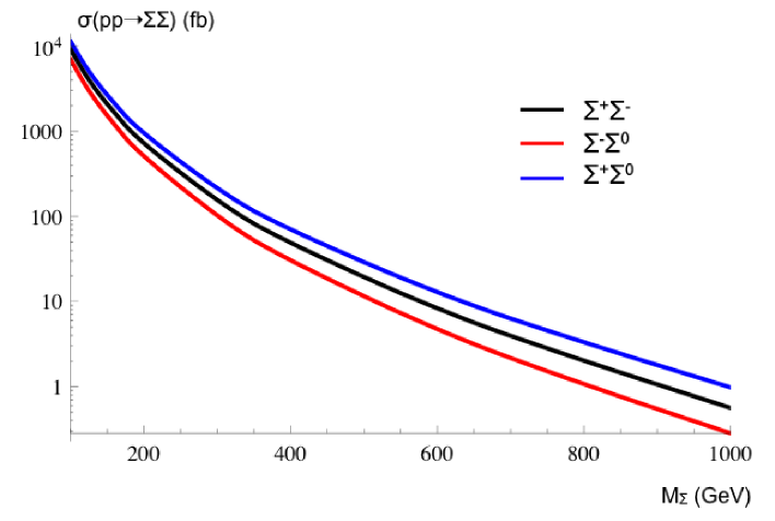
Figure 7: Production of a pair of triplets at 14 TeV at the LHC. The mixing parameters as been set to $V_{\mu}=0.063$ and $V_{e}=V_{\tau}=0$.

Appendix C Cross sections of the relevant channels at 7 TeV

Process	Cross Sections (fb)			Final State	Final State Cross Section (fb)
	100 GeV	120 GeV	140 GeV		100 GeV	120 GeV	140 GeV
Final State $++$
$W^{-}\mu^{+}Z\mu^{+}$	$2.36\rm{e}+2$	$2.02\rm{e}+2$	$1.16\rm{e}+2$	$\mu^{+}\mu^{+}hadr$	$108$	$92.7$	$53.4$
				$\mu^{+}\mu^{+}\nu\nu hadr$	$32.4$	$27.8$	$15.9$
$W^{-}\mu^{+}W^{+}\nu$	$1.66\rm{e}+3$	$6.06\rm{e}+2$	$2.82\rm{e}+2$	$\mu^{+}\mu^{+}\nu\nu hadr$	$124$	$45.3$	$21.1$
$W^{-}\mu^{+}h\mu^{+}$	$1.22\rm{e}-3$	$1.39\rm{e}-1$	$1.40\rm{e}+1$	$\mu^{+}\mu^{+}hadr$	-	-	$8.9$
				$\mu^{+}\mu^{+}\nu\nu hadr$	-	-	-
Total Cross Sections $\mu^{+}\mu^{+}$ + jets + missing $E_{T}$					156.4	73.1	37.0
Total Cross Sections $\mu^{+}\mu^{+}$ + jets					108	92.7	62.3
Final State $--$
$W^{+}\mu^{-}Z\mu^{-}$	$1.27\rm{e}+2$	$1.04\rm{e}+2$	$5.67\rm{e}+1$	$\mu^{-}\mu^{-}hadr$	$58.3$	$47.7$	$26.1$
				$\mu^{-}\mu^{-}\nu\nu hadr$	$17.4$	$14.3$	$7.8$
$W^{+}\mu^{-}W^{-}\nu$	$8.94\rm{e}+2$	$3.11\rm{e}+2$	$1.39\rm{e}+2$	$\mu^{-}\mu^{-}\nu\nu hadr$	$67.0$	$23.3$	$10.4$
$W^{+}\mu^{-}h\mu^{-}$	$5.87\rm{e}-6$	$7.13\rm{e}-2$	$6.86$	$\mu^{-}\mu^{-}hadr$	-	-	$4.4$
				$\mu^{-}\mu^{-}\nu\nu hadr$	-	-	-
Total Cross Sections $\mu^{-}\mu^{-}$ + jets + missing $E_{T}$					84.4	37.6	18.2
Total Cross Sections $\mu^{-}\mu^{-}$ + jets					58.3	47.7	30.5

Table 7: Final states with two muons of the same sign for $V_{e}=V_{\tau}=0$, $V_{\mu}=0.063$. The final cross sections have been computed using the measured branching ratios, except for the Higgs, whose branching ratios have been calculated assuming a mass of 120 GeV. Only channels with a final cross section higher than 0.1 have been reported.

Process	Cross Sections (fb)			Final State	Final State Cross Section (fb)
	100 GeV	120 GeV	140 GeV		100 GeV	120 GeV	140 GeV
Final State $++-$
$W^{+}\mu^{-}W^{+}\nu$	$1.66\rm{e}+3$	$6.08\rm{e}+2$	$2.82\rm{e}+2$	$\mu^{+}\mu^{+}\mu^{-}\nu\nu\nu$	$20.9$	$7.7$	$3.5$
$W^{-}\mu^{+}W^{+}\nu$	$1.66\rm{e}+3$	$6.06\rm{e}+2$	$2.82\rm{e}+2$	$\mu^{+}\mu^{+}\mu^{-}\nu\nu\nu$	$20.9$	$7.7$	$3.5$
$W^{+}\mu^{-}Z\mu^{+}$	$2.36\rm{e}+2$	$2.03\rm{e}+2$	$1.16\rm{e}+2$	$\mu^{+}\mu^{+}\mu^{-}\nu hadr$	$18.2$	$15.7$	$8.9$
				$\mu^{+}\mu^{+}\mu^{-}\nu\nu\nu$	$5.5$	$4.7$	$2.7$
$W^{-}\mu^{+}Z\mu^{+}$	$2.36\rm{e}+2$	$2.02\rm{e}+2$	$1.16\rm{e}+2$	$\mu^{+}\mu^{+}\mu^{-}\nu hadr$	$18.3$	$15.6$	$8.9$
				$\mu^{+}\mu^{+}\mu^{-}\nu\nu\nu$	$5.5$	$4.6$	$2.6$
$W^{+}\nu Z\nu$	$4.62\rm{e}+2$	$4.02\rm{e}+2$	$2.32\rm{e}+2$	$\mu^{+}\mu^{+}\mu^{-}\nu\nu\nu$	$1.8$	$1.6$	$0.9$
$Z\mu^{+}Z\nu$	$6.55\rm{e}+1$	$1.35\rm{e}+2$	$9.48\rm{e}+1$	$\mu^{+}\mu^{+}\mu^{-}\nu hadr$	$1.6$	$3.2$	$2.3$
				$\mu^{+}\mu^{+}\mu^{-}\nu\nu\nu$	$0.47$	$0.98$	$0.68$
$Z\mu^{+}h\nu$	$6.80\rm{e}-4$	$1.54\rm{e}-1$	$2.28\rm{e}+1$	$\mu^{+}\mu^{+}\mu^{-}\nu hadr$	-	-	0.76
$W^{-}\nu Z\mu^{+}$	$3.61\rm{e}+2$	$3.08\rm{e}+2$	$1.71\rm{e}+2$	$\mu^{+}\mu^{+}\mu^{-}\nu hadr$	$8.4$	$7.2$	$4.0$
$W^{+}\mu^{-}h\mu^{+}$	$1.22\rm{e}-3$	$1.39\rm{e}-1$	$1.40\rm{e}+1$	$\mu^{+}\mu^{+}\mu^{-}\nu hadr$	-	-	$1.5$
$W^{-}\mu^{+}h\mu^{+}$	$1.22\rm{e}-3$	$1.39\rm{e}-1$	$1.40\rm{e}+1$	$\mu^{+}\mu^{+}\mu^{-}\nu hadr$	-	-	1.5
Total Cross Sections $\mu^{+}\mu^{+}\mu^{-}$ + jets + missing $E_{T}$					$46.5$	$41.7$	$27.9$
Total Cross Sections $\mu^{+}\mu^{+}\mu^{-}$ + jets + missing $E_{T}$ (only via W)					$36.5$	$31.3$	$20.8$
Total Cross Sections $\mu^{+}\mu^{+}\mu^{-}$ + missing $E_{T}$					$55.1$	$27.3$	$13.9$
Total Cross Sections $\mu^{+}\mu^{+}\mu^{-}$ + missing $E_{T}$ (only via W)					$52.8$	$24.7$	$12.3$
Final State $+--$
$W^{-}\mu^{+}W^{-}\nu$	$8.96\rm{e}+2$	$3.13\rm{e}+2$	$1.39\rm{e}+2$	$\mu^{-}\mu^{-}\mu^{+}\nu\nu\nu$	11.2	3.9	1.7
$W^{+}\mu^{-}W^{-}\nu$	$8.94\rm{e}+2$	$3.11\rm{e}+2$	$1.39\rm{e}+2$	$\mu^{-}\mu^{-}\mu^{+}\nu\nu\nu$	11.1	3.9	1.7
$W^{-}\mu^{+}Z\mu^{-}$	$1.27\rm{e}+2$	$1.04\rm{e}+2$	$5.67\rm{e}+1$	$\mu^{-}\mu^{-}\mu^{+}\nu hadr$	9.8	8.0	4.4
				$\mu^{-}\mu^{-}\mu^{+}\nu\nu\nu$	2.9	2.4	1.3
$W^{+}\mu^{-}Z\mu^{-}$	$1.27\rm{e}+2$	$1.04\rm{e}+2$	$5.67\rm{e}+1$	$\mu^{-}\mu^{-}\mu^{+}\nu hadr$	9.8	8.0	4.4
				$\mu^{-}\mu^{-}\mu^{+}\nu\nu\nu$	2.9	2.4	1.3
$W^{-}\nu Z\nu$	$2.49\rm{e}+2$	$2.07\rm{e}+2$	$1.13\rm{e}+2$	$\mu^{-}\mu^{-}\mu^{+}\nu\nu\nu$	1.0	0.8	0.4
$Z\mu^{-}Z\nu$	$3.53\rm{e}+1$	$6.93\rm{e}+1$	$4.65\rm{e}+1$	$\mu^{-}\mu^{-}\mu^{+}\nu hadr$	0.85	1.7	1.1
				$\mu^{-}\mu^{-}\mu^{+}\nu\nu\nu$	0.25	0.5	0.3
$Z\mu^{-}h\nu$	$3.27\rm{e}-4$	$7.87\rm{e}-2$	$1.12\rm{e}+1$	$\mu^{-}\mu^{-}\mu^{+}\nu hadr$	-	-	$0.37$
$W^{+}\nu Z\mu^{-}$	$3.62\rm{e}+2$	$3.07\rm{e}+2$	$1.72\rm{e}+2$	$\mu^{-}\mu^{-}\mu^{+}\nu hadr$	$8.4$	$7.2$	$4.0$
$W^{-}\mu^{+}h\mu^{-}$	$5.87\rm{e}-4$	$7.13\rm{e}-2$	$6.86$	$\mu^{-}\mu^{-}\mu^{+}\nu hadr$	-	-	$0.7$
$W^{+}\mu^{-}h\mu^{-}$	$5.86\rm{e}-4$	$7.10\rm{e}-2$	$6.87$	$\mu^{-}\mu^{-}\mu^{+}\nu hadr$	-	-	0.7
Total Cross Sections $\mu^{+}\mu^{-}\mu^{-}$ + jets + missing $E_{T}$					$28.9$	$24.9$	$15.7$
Total Cross Sections $\mu^{+}\mu^{-}\mu^{-}$ + jets + missing $E_{T}$ (only via W)					$19.6$	$16.0$	$10.2$
Total Cross Sections $\mu^{+}\mu^{-}\mu^{-}$ + missing $E_{T}$					$29.4$	$13.9$	$6.7$
Total Cross Sections $\mu^{+}\mu^{-}\mu^{-}$ + missing $E_{T}$ (only via W)					$28.1$	$12.6$	$6.0$

Table 8: Final states with three muons for $V_{e}=V_{\tau}=0$, $V_{\mu}=0.063$. The final cross sections have been computed using the measured branching ratios, except for the Higgs, whose branching ratios have been calculated assuming a mass of 120 GeV. Only channels with a final cross section higher than 0.1 have been reported. As for the total cross sections, we have isolated the ones where the muons are generated via $W$ decay, since almost all the muons generated via $Z$ decay will be removed by the cut implemented to reduce the $Z$ background.

References

- [1] N. D. Christensen and C. Duhr, Comput. Phys. Commun. 180 (2009) 1614 [arXiv:0806.4194 [hep-ph]].
- [2] J. Alwall et al., JHEP 0709 (2007) 028, [arXiv:0706.2334 [hep-ph]]; J. Alwall, M. Herquet, F. Maltoni, O. Mattelaer, T. Stelzer, JHEP 1106 (2011) 128, [arXiv:1106.0522 [hep-ph]].
- [3] P. Minkowski, Phys. Lett. B 67 421 (1977); M. Gell-Mann, P. Ramond and R. Slansky, in Supergravity, edited by P. van Nieuwenhuizen and D. Freedman, (North-Holland, 1979), p. 315; T. Yanagida, in Proceedings of the Workshop on the Unified Theory and the Baryon Number in the Universe, edited by O. Sawada and A. Sugamoto (KEK Report No. 79-18, Tsukuba, 1979), p. 95; R.N. Mohapatra and G. Senjanović, Phys. Rev. Lett. 44 (1980) 912.
-
[4]
M. Magg and C. Wetterich,
Phys. Lett. B94 (1980) 61;
J. Schechter and J. W. F. Valle, Phys. Rev. D 22 (1980) 2227;
C. Wetterich, Nucl. Phys. B187 (1981) 343;
G. Lazarides, Q. Shafi and C. Wetterich, Nucl Phys. B181 (1981) 287;
R.N. Mohapatra and G. Senjanović, Phys. Rev. D23 (1981) 165. - [5] R. Foot, H. Lew, X.-G. He and G.C. Joshi, Z. Phys. C44 (1989) 441.
- [6] R. N. Mohapatra, Phys. Rev. Lett. 56 (1986) 561-563; R. N. Mohapatra, J. W. F. Valle, Phys. Rev. D34 (1986) 1642.
- [7] F. del Aguila and J. A. Aguilar-Saavedra, Nucl. Phys. B 813, 22 (2009) [arXiv:0808.2468 [hep-ph]].
- [8] R. Franceschini, T. Hambye and A. Strumia, Phys. Rev. D 78 (2008) 033002 [arXiv:0805.1613 [hep-ph]].
- [9] B. Bajc, G. Senjanovic, JHEP 0708 (2007) 014, [hep-ph/0612029]; B. Bajc, M. Nemevsek, G. Senjanovic, Phys. Rev. D76 (2007) 055011, [hep-ph/0703080]; A. Arhrib, B. Bajc, D. K. Ghosh, T. Han, G. -Y. Huang, I. Puljak, G. Senjanovic, Phys. Rev. D82 (2010) 053004, [arXiv:0904.2390 [hep-ph]].
- [10] A. Abada, C. Biggio, F. Bonnet, M. B. Gavela and T. Hambye, Phys. Rev. D 78 (2008) 033007 [arXiv:0803.0481 [hep-ph]].
- [11] K. Nakamura et al. [ Particle Data Group Collaboration ], J. Phys. G G37 (2010) 075021.
- [12] P. Meade and M. Reece, arXiv:hep-ph/0703031.
- [13] A. Abada, C. Biggio, F. Bonnet, M. B. Gavela and T. Hambye, JHEP 0712 (2007) 061 [arXiv:0707.4058 [hep-ph]].
- [14] F. del Aguila, J. de Blas, M. Perez-Victoria, Phys. Rev. D78 (2008) 013010. [arXiv:0803.4008 [hep-ph]].
- [15] T. Sjostrand, S. Mrenna, P. Z. Skands, JHEP 0605 (2006) 026. [hep-ph/0603175].
- [16] J. Conway et al., ”PGS4: Pretty Good Simulation of high energy collisions.” 2006. http://www.physics.ucdavis.edu/ conway/research/software/pgs/pgs4-general.htm
- [17] L. Basso, A. Belyaev, S. Moretti and C. H. Shepherd-Themistocleous, Phys. Rev. D 80 (2009) 055030 [arXiv:0812.4313 [hep-ph]]; L. Basso, arXiv:1106.4462 [hep-ph].
- [18] S. Chatrchyan et al. [ CMS Collaboration ], [arXiv:1102.4746 [hep-ex]].
- [19] S. Chatrchyan et al. [ CMS Collaboration ], [arXiv:1106.0902 [hep-ex]].
- [20] G. Aad et al. [ ATLAS Collaboration ], [arXiv:1108.3699 [hep-ex]].
- [21] S. Chatrchyan et al. [ CMS Collaboration ], Phys. Lett. B699 (2011) 25-47. [arXiv:1102.5429 [hep-ex]].
- [22] G. Aad et al. [ ATLAS Collaboration ], [arXiv:1104.5225 [hep-ex]].
- [23] [ CMS Collaboration ],“Measurement of the WW, WZ and ZZ cross sections at CMS”, CMS-EWK-11-010-PAS.
- [24] N. D. Christensen, P. de Aquino, C. Degrande, C. Duhr, B. Fuks, M. Herquet, F. Maltoni, S. Schumann, Eur. Phys. J. C71 (2011) 1541. [arXiv:0906.2474 [hep-ph]].