Homepage: ]http://www.smsyslab.org

Microcanonical entropy inflection points: Key to systematic understanding
of transitions in finite systems

Abstract

We introduce a systematic classification method for the analogs of phase transitions in finite systems. This completely general analysis, which is applicable to any physical system and extends towards the thermodynamic limit, is based on the microcanonical entropy and its energetic derivative, the inverse caloric temperature. Inflection points of this quantity signal cooperative activity and thus serve as distinct indicators of transitions. We demonstrate the power of this method through application to the long-standing problem of liquid-solid transitions in elastic, flexible homopolymers.

Structure formation processes are typically accompanied by nucleation transitions, where crystalline shapes form out of a liquid or vapor phase. Thus, nucleation is governed by finite-size and surface effects. For small physical systems, it is difficult to understand thermodynamic transitions of this type, as they strongly depend on system size.

Cooperativity refers to collective changes in a statistically significant fraction of the degrees of freedom in a system, which transforms the system into a new macrostate. In the thermodynamic limit of an infinitely large system, the ensemble of macrostates sharing similar thermodynamic properties would be called a “phase” and the transformation a “phase transition”. The description of such a transformation in a finite system is more subtle, as it cannot be described in the traditional Ehrenfest scheme of singularities in response quantities. However, statistical physics and thus thermodynamics are also valid for systems with no thermodynamic limit. Examples include the structure formation in small atomic clusters and all biomolecules. This is particularly striking for proteins, i.e., heterogeneous linear chains of amino acids. The fact that the individual biological function is connected with the geometrical shape of the molecule makes it necessary to discriminate unfolded (non-functional) and folded (functional) states. Although these systems are finite, they undergo a structural transition by passing a single (or more) free-energy barrier(s). Since these finite-system transitions exhibit strong similarities compared to phase transitions, we extend the terminology once defined in the thermodynamic limit to all systems exhibiting cooperative behavior.

In this paper, we introduce a commonly applicable and simple method for the identification and classification of cooperative behavior in systems of arbitrary size by means of microcanonical thermodynamics gross1 . It also includes the precise and straightforward analysis of the finite-size effects, which are important to a general understanding of the onset of phase transitions. This is in contrast to canonical approaches, where detailed information is lost by averaging out thermal fluctuations. Re-gaining information about finite-size effects in canonical schemes, e.g., by the investigation of the distribution of Lee-Yang zeros in the complex temperature plane borrmann or by inverse Laplace transform cohen1 , is complicated.

The identification of transitions is associated with a distinct definition of transition points such as a transition temperature. In the canonical representation of finite systems these usually differ, e.g., peak structures of thermodynamic quantities, such as the specific heat and fluctuations of order parameters as functions of the heat-bath temperature. This makes it impossible to fix a unique transition point. In the microcanonical analysis, the temperature is defined via the curvature of the caloric entropy curve and thus all transition signals in the microcanonical entropy can be directly associated with a transition temperature.

After introducing the method, we apply it to liquid-solid and solid-solid transitions occurring for elastic, flexible polymers, which have been under debate for quite some time. In contrast to the rather well-understood coil-globule collapse transition, the formation of highly compact crystalline, amorphous, or glasslike structures intricately depends on the precise relation of intrinsic energy and length scales in the system binder0 ; vbj1 ; seaton1 ; sbj1 ; taylor1 ; seaton3 .

In recent work, the microcanonical analysis has successfully been applied in aggregation studies of coarse-grained polymer and peptide models, where a nucleation process was found to be an energetically ordered hierarchy of individual structural subphase transitions jbj1 . Caloric approaches have also been used to investigate the folding behavior of proteins liang1 ; gomez1 ; b1 ; bbd1 ; bdb1 and the structural phases of polymers with stiff bonds taylor1 , as well as polymer adsorption transitions bj1 ; liang3 ; mjb1 . Other applications include the formation of galaxies thirring1 , the clustering and fragmentation of atomic clusters and nuclei gross1 ; gross2 ; doye1 , and order–disorder transitions in spin systems gross1 ; wj1 ; hueller1 ; cohen1 ; pleimling1 . Most of these studies are aimed at using the microcanonical analysis as an alternative approach to investigating finite-size scaling properties. However, a systematic scheme for the classification of transitions in the respective finite systems has remained lacking. The method introduced here closes this gap through the introduction of an Ehrenfest-like analysis based on microcanonical entropy inflection points.

A fundamental property of each physical system, and the central quantity for our method, is the microcanonical entropy $S(E)=k_{B}\ln g(E)$, where $g(E)$ is the density of states for a given energy $E$ (in the following, we will set $k_{B}\equiv 1$). Alternatively, a volume entropy can be defined via the integrated density of states by $S^{\prime}(E)=k_{B}\ln G(E)$ with $G(E)=\int_{E_{\rm min}}^{E}dE^{\prime}g(E^{\prime})$ hertz1 , which is virtually identical with $g(E)\Delta E$ ($|\Delta E/E|\ll 1$) in the transition regions jbj1 . It has been argued that only $G(E)$ is consistent with the classical equipartition theorem tiller1 ; campisi1 , however, its physical meaning is much less obvious gross1 . Therefore, we will continue using $S(E)$ instead. It should also be mentioned that $g(E)$ is the “natural” output provided, e.g., by generalized-ensemble Monte Carlo methods. Among the most prominent of these methods are multicanonical muca and Wang-Landau wl sampling, which enable a precise numerical estimation of this quantity over hundreds or even thousands of orders of magnitude sbj1 ; seaton1 .

A qualitative change in the interplay of entropy and energy in the system is signaled by noticeable alterations in the curvature of $S(E)$, which are quantitative measures for the strength of cooperativity of the associated transitions. For finite systems exhibiting transitions with phase separation, $S(E)$ can even possess convex regions gross1 , although it is a strictly concave function in the thermodynamic limit. In this case, the slope of a tangent at each point of the curve is unique, and it is common to define the reciprocal microcanonical temperature via the caloric derivative of $S$,

$$\beta(E)\equiv T^{-1}(E)=(dS/dE)_{N,V}~{},$$ (1)

where system size $N$ and volume $V$ are kept constant. In the thermodynamic limit, where fluctuations about the mean energy become negligible, the canonical and microcanonical ensembles are identical, and the canonical (or heat-bath) temperature equals the microcanonical temperature. This is not the case for a finite system experiencing a structural transition, where different quantities vary in their fluctuation properties, rendering an identification of transition points impossible. Since the complete phase behavior is already encoded in $S(E)$, it is useful to consider $\beta(E)$ as a unique parameter to identify transition points.

We further propose to analyze the monotonic behavior of $\beta(E)$, expressed by its derivative with respect to energy,

$$\gamma(E)=d\beta(E)/dE=d^{2}S/dE^{2}.$$ (2)

This will allow for the introduction of a systematic classification scheme of transitions in finite systems. In principle, this can also be used for scaling analyses towards the thermodynamic limit.

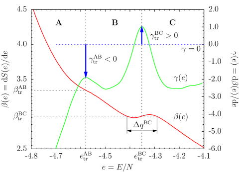
Figure 1: (Color online) Inverse temperature $\beta(e)$ and its derivative $\gamma(e)$ as functions of the energy per particle, $e=E/N$, exemplified for an elastic polymer with 102 monomers. The maxima of $\gamma(e)$ indicate transitions between the structural phases A and B at $e_{\rm tr}^{\rm AB}$ and B and C at $e_{\rm tr}^{\rm BC}$. The associated points $\beta(e_{\rm tr}^{\rm AB})=\beta_{\rm tr}^{\rm AB}$ and $\beta(e_{\rm tr}^{\rm BC})=\beta_{\rm tr}^{\rm BC}$ define the transition temperatures $T_{\rm tr}^{\rm AB}=(\beta_{\rm tr}^{\rm AB})^{-1}$ and $T_{\rm tr}^{\rm BC}=(\beta_{\rm tr}^{\rm BC})^{-1}$. According to our classification scheme, the transition between A and B is of second order, since the slope of the inflection point is negative. On the other hand, B$\leftrightarrow$C is a first-order transition as the respective slope at $\beta(e_{\rm tr}^{\rm BC})$ is positive. The non-monotonicity of $\beta(e)$ in this region, called “backbending”, is a typical signal of phase coexistence. The latent heat $\Delta q^{\rm BC}$ is defined as the energetic width of this transition region.

We define a transition between phases to be of first order if the slope of the corresponding inflection point of $\beta(E)$ at $E=E_{\rm tr}$ is positive, i.e., $\gamma_{\rm tr}=\gamma(E_{\rm tr})>0$. Only in this case is the temperature curve non-monotonic and there is no unique mapping between $\beta$ and $E$. Physically, both phases coexist in the transition region. The overall energetic width of the undercooling, backbending, and overheating regions, obtained from a Maxwell construction, is thus identical to the latent heat. Therefore, for a first-order transition, $\Delta q>0$. In the case that the inflection point has a negative slope, $\gamma_{\rm tr}=\gamma(E_{\rm tr})<0$, the phases cannot coexist and the latent heat is zero. In complete analogy to phase transitions in the thermodynamic limit, we classify such transitions as of second order. Since the inflection points of $\beta(E)$ correspond to maxima in $\gamma(E)$, it is therefore sufficient to analyze the peak structure of $\gamma(E)$ in order to identify the transition energies and temperatures. The sign of the peak values classifies the transition. This very simple and general classification scheme applies to all physical systems.

Figure 1 illustrates the procedure for the identification of the transitions by means of inflection-point analysis, where the inverse temperature $\beta$ and its energetic derivative $\gamma$ are plotted as functions of the reduced energy $e=E/N$, with $N$ being the system size. As a first example, we consider an elastic flexible homopolymer with $N=102$ monomers. This system exhibits four structural phases sbj1 : two solid icosahedral phases (A: Mackay, B: anti-Mackay), a globular liquid phase (C), and the random-coil phase (D). In Fig. 1, the transitions can indeed be uniquely identified (since the C$\leftrightarrow$D transition occurs at much higher energy and temperature, it is not included, but can also easily be found by inflection-point analysis; it is a second-order transition at $e_{\rm tr}^{\rm CD}\approx-1.21$, $\beta_{\rm tr}^{\rm CD}\approx 1.08$). A 1^st-order liquid-solid transition B$\leftrightarrow$C is characterized by $\gamma_{\rm tr}^{\rm BC}>0$ at $e_{\rm tr}^{\rm BC}\approx-4.35$ ($\beta_{\rm tr}^{\rm BC}\approx 2.97$). The width of the energetic transition region corresponds to the latent heat, $\Delta q^{\rm BC}$, which is obviously nonzero because of the backbending effect or the coexistence of both phases in this region. The 2^nd-order transition A$\leftrightarrow$B is found at $e_{\rm tr}^{\rm AB}\approx-4.58$ ($\beta_{\rm tr}^{\rm AB}\approx 3.34$) by an inflection point with negative slope ($\gamma_{\rm tr}^{\rm AB}<0$).

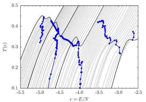
Figure 2: (Color online) Caloric temperature curves $T(e)=\beta^{-1}(e)$ for a selection of elastic, flexible polymers with chain lengths in the interval $N=13,\ldots,309$ (from right to left). Curves for chains with magic length ($N=13,55,147,309$) are bold. The relevant inflection points, indicating the conformational transitions on the basis of our analysis method, are marked by $\bullet$ symbols.

In order to demonstrate the capability of our method to systematically analyze all transitions in finite systems, we estimate the transition points for the entire set of elastic Lennard-Jones homopolymers with $N=13,\ldots,309$ monomers. In the liquid and solid regimes, the structural behavior of these polymers is very similar to rare-gas systems consisting of $N$ atoms, which also form compact, crystalline clusters at very low temperatures frant1 ; sbj1 ; seaton3 . We employ the standard model for flexible, elastic polymers, where the monomers interact via a truncated-shifted Lennard-Jones potential, $E_{\rm LJ}^{\rm mod}(r_{ij})=E_{\rm LJ}(\min(r_{ij},r_{\rm c}))-E_{\rm LJ}(r_{\rm c})$ with $E_{\rm LJ}(r_{ij})=4\epsilon[(\sigma/r_{ij})^{12}-(\sigma/r_{ij})^{6}]$, where $r_{ij}$ is the distance between two monomers located at ${\bf r}_{i}$ and ${\bf r}_{j}$ ($i,j=1,\ldots,N$), and $\epsilon=1$ and $\sigma=2^{-1/6}r_{0}$, with the potential minimum at $r_{0}=0.7$ and the cutoff at $r_{\rm c}=2.5\sigma$. Adjacent monomers are connected by finitely extensible nonlinear elastic (FENE) anharmonic bonds FENE ; binder3 , $E_{\rm FENE}(r_{i\,i+1})=-KR^{2}\ln\{1-[(r_{i\,i+1}-r_{0})/R]^{2}\}^{1/2}$. The FENE potential minimum is located at $r_{0}$ and diverges for $r\rightarrow r_{0}\pm R$ (in our simulations $R=0.3$). The spring constant $K$ is set to $40$. The total energy of a polymer conformation ${\bf X}=({\bf r}_{1},\ldots,{\bf r}_{N})$ is given by $E({\bf X})=\sum_{i=1}^{N}\sum_{j=i+1}^{N}E^{\rm mod}_{\rm LJ}(r_{ij})+\sum_{i=1}^{N-1}E_{\rm FENE}(r_{ii+1}).$

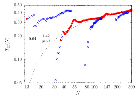
Figure 3: (Color online) Transition temperatures $T_{\rm tr}(N)$ of conformational transitions for small elastic polymers with chain lengths $N=13,\ldots,309$ in the liquid-solid and solid-solid transition regimes, obtained from inflection-point analysis. First-order transition points are marked by red symbols ($\bullet$), second-order transition points by blue symbols ($\times$). Also shown is a fit for the liquid-solid transition temperature towards the thermodynamic limit $N\to\infty$ (dashed line).

Figure 2 shows the caloric temperature curves for elastic polymers with various chain lengths in the liquid and solid regimes, calculated from highly accurate density of states estimates obtained in sophisticated multicanonical Monte Carlo simulations sjb1 . The identified inflection points associated with conformational transitions are indicated by $\bullet$ symbols. As expected, there is no general and obvious relation of the behavior of chains with slightly different lengths. This is due to the still dominant finite-size effects of the polymer trying to reduce their individual surface-to-volume ratio, which therefore strongly depends on optimal monomer packings in the interior and on the surface of the conformations. For example, for chains of moderate lengths ($N\leq 147$ sbj1 ; seaton3 ), the different behavior can be traced back to the monomer arrangements on the facets of icosahedral structures, known as Mackay and anti-Mackay overlayers northby1 . Solid-solid transitions between Mackay and anti-Mackay structures are also possible under certain conditions in these systems sbj1 ; seaton3 . This can be seen in Fig. 3, where all transition temperatures $T_{\rm tr}(N)=\beta^{-1}_{\rm tr}(N)$ for liquid-solid and solid-solid transitions are plotted in dependence of the chain length $N$ rem1 . Symbols $\bullet$ indicate first-order transitions, which for $N>38$ can be associated to the respective liquid-solid transitions, whereas symbols $\times$ mark second-order transitions.

If the associated transition temperatures are smaller than the liquid-solid transition temperatures, the symbols indicating second-order behavior belong to solid-solid transitions, e.g., transitions between geometrical shapes with Mackay or anti-Mackay overlayers. Note the different behavior for “magic” chain lengths $N_{\rm magic}=13,55,147,309,\ldots$, in which icosahedral Mackay ground states form. Figure 3 also gives evidence for the convergence of the solid-solid and liquid-solid transition temperatures when $N$ approaches a magic length. This behavior repeats for each $N$ interval that finally ends at a certain magic length $N_{\rm magic}$, where both transitions merge into a single first-order liquid-solid transition. The influence of the solid-solid effects weakens with increasing system size, while the liquid-solid transition remains a true phase transition in the thermodynamic limit. Inserted into the plot is a fit function $T_{\rm tr}(N)=T^{\rm ls}-aN^{-1/3}$ which suggests an estimate for the thermodynamic phase transition temperature $T_{\rm tr}^{\rm ls}\approx 0.64$.

Summarizing, we have introduced a general method for the analysis of phase transitions in small systems based on the central quantity of any statistical system, the microcanonical entropy, and applied it to the long-standing problem of structural transitions of flexible polymers. Advanced Monte Carlo simulation techniques such as multicanonical sampling muca and the Wang-Landau method wl enable precise estimations of the density of states, and thus it is straightforward to obtain the microcanonical entropy in computer simulations. Since indicative quantities such as transition temperatures can be quantitatively determined, our method also enables experimentally competitive predictions.

This project has been partially supported by NSF DMR-0810223.

References

- (1) D. H. E. Gross, Microcanonical Thermodynamics (World Scientific, Singapore, 2001).
- (2) P. Borrmann, O. Mülken, and J. Harting, Phys. Rev. Lett. 84, 3511 (2000); O. Mülken, H. Stamerjohanns, and P. Borrmann, Phys. Rev. E 64, 047105 (2001).
- (3) I. Ispolatov and E. G. D. Cohen, Physica A 295, 475 (2001).
- (4) F. Rampf, W. Paul, K. Binder, Europhys. Lett. 70, 628 (2005); J. Polym. Sci.: Part B: Polym. Phys. 44, 2542 (2006); W. Paul, T. Strauch, F. Rampf, and K. Binder, Phys. Rev. E 75, 060801(R) (2007).
- (5) T. Vogel, M. Bachmann, and W. Janke, Phys. Rev. E 76, 061803 (2007).
- (6) D. T. Seaton, S. J. Mitchell, and D. P. Landau, Braz. J. Phys. 38, 48 (2008); D. T. Seaton, T. Wüst, and D. P. Landau, Comp. Phys. Comm. 180, 587 (2009).
- (7) S. Schnabel, T. Vogel, M. Bachmann, and W. Janke, Chem. Phys. Lett. 476, 201 (2009); S. Schnabel, M. Bachmann, and W. Janke, J. Chem. Phys. 131, 124904 (2009).
- (8) M. P. Taylor, W. Paul, and K. Binder, Phys. Rev. E 79, 050801(R) (2009); J. Chem. Phys. 131, 114907 (2009).
- (9) D. T. Seaton, T. Wüst, and D. P. Landau, Phys. Rev. E 81, 011802 (2010).
- (10) C. Junghans, M. Bachmann, and W. Janke, Phys. Rev. Lett. 97, 218103 (2006); J. Chem. Phys. 128, 085103 (2008); Europhys. Lett. 87, 40002 (2009).
- (11) T. Chen, X. S. Lin, Y. Liu, and H. J. Liang, Phys. Rev. E 76, 046110 (2007); Phys. Rev. E 78, 056101 (2008).
- (12) J. Hernández-Rojas and J. M. Gomez-Llorente, Phys. Rev. Lett. 100, 258104 (2008).
- (13) M. Bachmann, Phys. Proc. 3, 1387 (2010).
- (14) T. Bereau, M. Bachmann, and M. Deserno, J. Am. Chem. Soc. 132, 13129 (2010).
- (15) T. Bereau, M. Deserno, and M. Bachmann, Biophys. J. in press (2011).
- (16) M. Bachmann and W. Janke, Phys. Rev. Lett. 95, 058102 (2005); Phys. Rev. E 73, 041802 (2006); Lect. Notes Phys. 736, 203 (2008).
- (17) L. Wang, T. Chen, X. S. Lin, Y. Liu, and H. J. Liang, J. Chem. Phys. 131, 244902 (2009).
- (18) M. Möddel, W. Janke, and M. Bachmann, Phys. Chem. Chem. Phys., 12, 11548 (2010).
- (19) W. Thirring, Z. Physik 235, 339 (1970).
- (20) D. H. E. Gross and J. F. Kenney, J. Chem. Phys. 122, 224111 (2005).
- (21) E. G. Noya and J. P. K. Doye, J. Chem. Phys. 124, 104503 (2006).
- (22) W. Janke, Nucl. Phys. B (Proc. Suppl.) 63A-C, 631 (1998).
- (23) M. Kastner, M. Promberger, and A. Hüller, J. Stat. Mech. 99, 1251 (2000).
- (24) H. Behringer and M. Pleimling, Phys. Rev. E 74, 011108 (2006); H. Behringer, Entropy 10, 224 (2008).
- (25) P. Hertz, Ann. Phys. 33, 225 (1910); ibid., 537 (1910).
- (26) E. M. Pearson, T. Halicioglu, and W. A. Tiller, Phys. Rev. A 32, 3030 (1985).
- (27) M. Campisi and D. H. Kobe, Am. J. Phys. 78, 608 (2010).
- (28) B. A. Berg and T. Neuhaus, Phys. Lett. B 267, 249 (1991); Phys. Rev. Lett. 68, 9 (1992).
- (29) F. Wang and D. P. Landau, Phys. Rev. Lett. 86, 2050 (2001); Phys. Rev. E 64, 056101 (2001); Comp. Phys. Commun. 147, 674 (2002).
- (30) P. A. Frantsuzov and V. A. Mandelshtam, Phys. Rev. E 72, 037102 (2005).
- (31) R. B. Bird, C. F. Curtiss, R. C. Armstrong, and O. Hassager, Dynamics of Polymeric Liquids, 2nd ed., 2 vols. (Wiley, New York, 1987).
- (32) A. Milchev, A. Bhattacharaya, and K. Binder, Macromolecules 34, 1881 (2001).
- (33) S. Schnabel, W. Janke, and M. Bachmann, J. Comput. Phys. 230, 4454 (2011).
- (34) J. A. Northby, J. Chem. Phys. 87, 6166 (1987).
- (35) The inflection-point analysis for can also easily be applied to the coil-globule transition, which occurs at much higher temperatures (for this reason, transition points are not inserted in Fig. 3).