Computing Heavy Elements

Abstract

Reliable calculations of the structure of heavy elements are crucial to address fundamental science questions such as the origin of the elements in the universe. Applications relevant for energy production, medicine, or national security also rely on theoretical predictions of basic properties of atomic nuclei. Heavy elements are best described within the nuclear density functional theory (DFT) and its various extensions. While relatively mature, DFT has never been implemented in its full power, as it relies on a very large number ($\sim 10^{9}-10^{12}$) of expensive calculations ($\sim$ day). The advent of leadership-class computers, as well as dedicated large-scale collaborative efforts such as the SciDAC 2 UNEDF project, have dramatically changed the field. This article gives an overview of the various computational challenges related to the nuclear DFT, as well as some of the recent achievements.

1 Introduction

Nuclear physics pervades a number of scientific disciplines as well as societal applications. Understanding the production of the elements in stellar interiors is key to reproduce the observed isotopic abundances in the universe. It necessitates an accurate knowledge of the structure of radioactive nuclides that are so short-lived that they will remain beyond reach of experimental facilities for many years to come, if not for ever. In the long term, the safety and viability of nuclear energy production sources will be enhanced by acquiring a precise understanding of the complex mechanisms of fission and fusion. The latter are also critical for stockpile stewardship, which has broad implications for national security.

At the heart of these important issues lies the elusive structure of the atomic nucleus. From a physics standpoint, it is a quantum many-body problem facing three major theoretical challenges: (1) the interaction that binds neutrons and protons together in the nucleus is in principle derived from quantum chromodynamics (QCD), but this derivation has not been firmly established yet; (2) the interaction between nucleons inside the nucleus is very different from the one between isolated nucleons in the vacuum (in-medium interactions); (3) the number of constituents in the nucleus ($\sim$1–300) almost always forbids both exact analytical solutions, except for the lightest systems, as well as the use of statistical methods applicable to systems with a very large number of particles. In spite of these formidable difficulties, there has been significant progress over the past 50 years to address all these issues.

While there exist many excellent models for light nuclei, heavy elements can be described only by what is variously known as the nuclear self-consistent mean-field theory or, more recently, density functional theory (DFT) [1]. Since its inception in the 1950ies, DFT has reached a satisfactory level of maturity. Until now, however, computational limitations did not allow to implement the theory as originally designed, resulting in uncontrolled systematic errors, poor precision, and dubious reliability in regions of exotic nuclei where experimental information is scarce or nonexistent. The fast development of leadership-class computers has for the first time lifted many of these limitations, and the solution to long-standing problems seems now possible in the short term. After briefly introducing the underlying theoretical background, this article discusses some of the computational challenges and methods used in nuclear DFT, highlights some of the recent achievements, and discusses current open problems.

2 Theoretical Models of Heavy Nuclei

The central hypothesis of nuclear DFT is that the $A$ nucleons (protons and neutrons) inside the nucleus can be treated as independent quasi-particles moving in an average nuclear potential well. The theory can be entirely formulated by introducing the so-called one-body density matrix $\rho(x,x^{\prime})$ and pairing tensor $\kappa(x,x^{\prime})$, where $x\equiv(\boldsymbol{r},\sigma)$ includes spatial as well as spin coordinates, $\sigma=\pm 1/2$. Requiring that the total energy $E$ of the nucleus is minimal under a variation of both $\rho$ and $\kappa$ leads to the so-called Hartree-Fock-Bogoliubov (HFB) equations:

$$\int dx^{\prime}\left(\begin{array}[]{cc}h[\rho(x,x^{\prime})]-\lambda&\Delta[\kappa(x,x^{\prime})]\\ -\Delta^{*}[\kappa(x,x^{\prime})]&-h^{*}[\rho(x,x^{\prime})]+\lambda\end{array}\right)\left(\begin{array}[]{c}U_{\mu}(x^{\prime})\\ V_{\mu}(x^{\prime})\end{array}\right)=E_{\mu}\left(\begin{array}[]{c}U_{\mu}(x)\\ V_{\mu}(x)\end{array}\right),\ \ \mu=1,\dots,+\infty,$$ (1)

with $\lambda$ a Lagrange parameter that must be introduced to conserve particle number, and

$$\begin{array}[]{l}\rho(x,x^{\prime})=\displaystyle\sum_{\mu}V_{\mu}^{*}(x)V_{\mu}(x^{\prime}),\vskip 6.0pt plus 2.0pt minus 2.0pt\\ \kappa(x,x^{\prime})=\displaystyle\sum_{\mu}V_{\mu}^{*}(x)U_{\mu}(x^{\prime}).\end{array}$$ (2)

In Eq. (1), $h[\rho]$ is a Hermitian operator (mean-field), which is a functional of the density matrix, and $\Delta[\kappa]$ is an antisymmetric operator (pairing field), which is a functional of the pairing tensor. The explicit dependence of the HFB matrix on the eigenfunctions $(U_{\mu},V_{\mu})$ via the density matrix and pairing tensor, or self-consistency, makes the eigenvalue problem highly nonlinear.

In its most general form, the mean-field operator reads:

$$h=-\frac{\hbar^{2}}{2m}\boldsymbol{\nabla}^{2}+\Gamma(x,x^{\prime})$$ (3)

with $\hbar$ the Planck constant, $m$ the mass of a nucleon, $\boldsymbol{\nabla}$ the gradient operator, and $\Gamma$ the so-called Hartree-Fock potential. In phenomenological mean-field models, $\Gamma$ is in fact parametrized by some suitable mathematical function and does not depend on the density matrix. In the traditional version of the self-consistent mean-field theory, $\Gamma$ is instead computed from a local two-body interaction, or effective pseudo-potential, $V(x,x^{\prime})$, which depends on the spatial and spin coordinates $x$ and $x^{\prime}$ of two nucleons and takes the general form

$$\Gamma(x,x^{\prime})=\delta(x-x^{\prime})\int dx_{1}V(x,x_{1})\rho(x_{1},x_{1})-V(x,x^{\prime})\rho(x,x^{\prime}).$$ (4)

Standard two-body interactions have either zero-range, that is, $V(x,x^{\prime})\sim\delta(\boldsymbol{r}-\boldsymbol{r}^{\prime})$ (Skyrme forces), or finite-range, $V(x,x^{\prime})\sim V(\boldsymbol{r}-\boldsymbol{r}^{\prime})$ (Gogny forces), which may further simplify the general expression (4). They all contain a density-dependent term that is necessary to reproduce the saturation of nuclear matter but that makes them ill-behaved for extensions of the theory dealing with large amplitude collective motion [2, 3]. Recent formulations of nuclear DFT do not consider explicitly effective interactions and instead parametrize $\Gamma(x,x^{\prime})$ directly as a functional of the density matrix $\rho(x,x^{\prime})$, or alternatively the local density $\rho(x)$ and its spatial derivatives.

The success of the nuclear mean-field theory relies on the mechanism of spontaneous symmetry breaking, whereby the solutions of the HFB equations (1) may break some of the symmetries of the underlying effective interaction $V(x,x^{\prime})$. This mechanism can be viewed as a way to introduce correlations in what is otherwise an independent particle model. A simple example is the breaking of rotational invariance of $V(x,x^{\prime})$, which implies that the density matrix and pairing tensor can have nonisotropic spatial distributions: in the mean-field theory, nuclei can be deformed, and the energy of the nucleus therefore depends on the deformation. However, this dependence is not known beforehand. In practice, one must introduce constraint operators $\hat{Q}_{lm}$ to probe the deformation energy surface. The problem is complicated by the fact that the expectation value $\langle Q_{lm}\rangle$ of the (local) constraint operator $\hat{Q}_{lm}$ is itself a functional of the density matrix,

$$\langle Q_{lm}\rangle=\int dx\hat{Q}_{lm}(x)\rho(x,x).$$ (5)

The HFB equations (1) with the constraints (5) represent a system of coupled, nonlinear, integro-differential equations and are the cornerstone of the description of heavy elements in a microscopic framework. In the following, we discuss the various methods used to solve these equations, as well as the related mathematical and computational challenges.

3 Mathematical and Computational Challenges

From a computational perspective, nuclear DFT has two facets: (i) the HFB solver itself and (ii) the management of a large number of quasi-independent, time-consuming, load-imbalanced tasks. We discuss below each of these aspects.

3.1 HFB Solver

Solving the HFB Equations - There exist essentially two classes of methods to solve the HFB equations. In the coordinate representation, the equations (1) are solved directly by numerical integration for each eigenfunction $\mu$. Boundary conditions for the wave-functions are imposed on the domain of integration. While precise, the feasibility and usability of this approach are highly dependent on the symmetries of the wave functions: in spherical symmetry, the eigenfunctions are separable $(U_{\mu}(\boldsymbol{r}),V_{\mu}(\boldsymbol{r}))=(u_{\mu}(r),v_{\mu}(r))Y_{lm}(\theta,\varphi)$. The HFB equations depend only on the radial coordinate $r$, and numerical implementations can be very fast (typically less than 1 minute per HFB calculation) [4]. In cylindrical symmetry, the wave-functions depend explicitly on the two variables $z$ and $\rho$, and special separation techniques (B-splines or similar) must be employed. Codes with built-in parallel capabilities achieve good convergence for a few dozens of cores/HFB calculation in a few hours [5]. Full 3D solvers in coordinate space are in development: they will probably require a large number of cores ($>$1,000) to achieve convergence in less than a day. At this scale, the benefits of using DFT (reformulate the problem to replace the $3A$ coordinates of the nucleons by the only three coordinates of the density matrix) are greatly reduced though.

The alternative approach consists of introducing a basis of the Hilbert space $\mathcal{L}_{2}$ of square-integrable functions and computing the matrix elements of all relevant operators in that basis. The Harmonic Oscillator (HO) basis proves the most adapted to nuclear structure applications as it involves very localized basis functions. By comparison, molecular physics applications often employ the plane wave basis. The choice of the coordinate system is dictated by the symmetries that one wants to impose, or relax, on the system. For example, fission studies typically require many spatial symmetries to be broken, and the Cartesian HO basis becomes the tool of choice. The HO basis is by definition an infinite countable basis of the one-particle Hilbert space: numerical implementations require the truncation of the expansion up to a maximum number of oscillator shells $N$. This introduces systematic truncation errors, as well as an artificial dependence on the frequency $\omega_{0}$ of the HO. When studying very deformed nuclei, it is recommended to choose an anisotropic 2D HO, with $\omega_{\perp}\neq\omega_{\parallel}$. The final truncation error then depends also on the deformation of the basis, that is, the ratio $q=\omega_{\parallel}/\omega_{\perp}$. For any practical calculation, the final HFB energy $E$ should therefore be written $E(N,\omega_{0},q)$. High-precision calculations require systematic and costly studies of this model space dependence; see Figs. 2–2 [6]. Recent attempts have therefore been made to apply multiresolution methods based on wavelet expansions to nuclear DFT, in order to combine the versatility of basis expansion with arbitrary precision results [7].

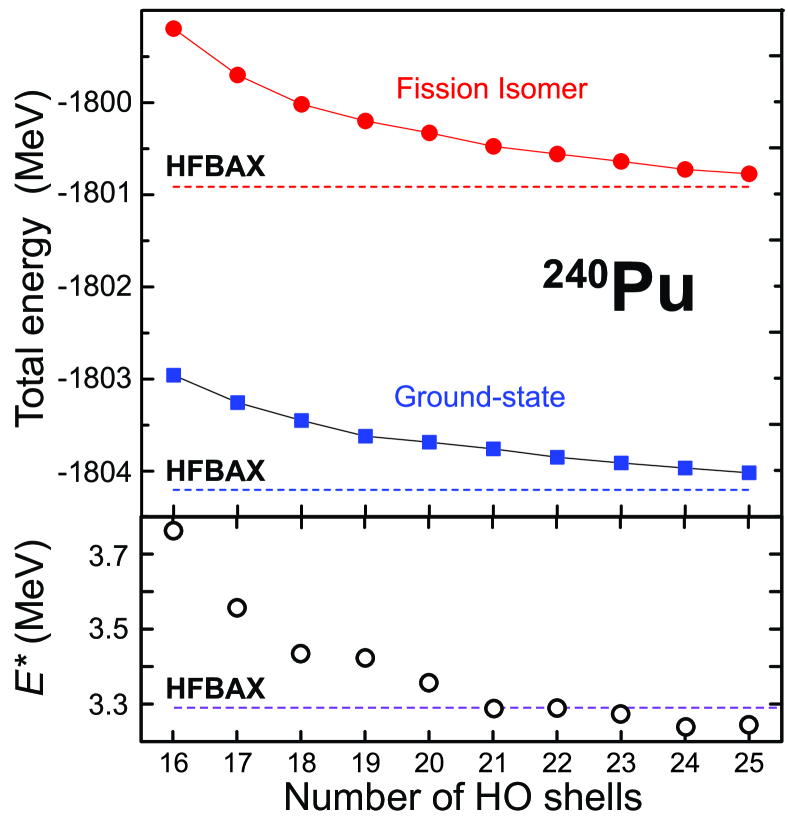
Figure 1: (color online) Convergence of the energy for various deformed states in ²⁴⁰Pu as function of the number of HO shells. The dashed line gives the result of [5].

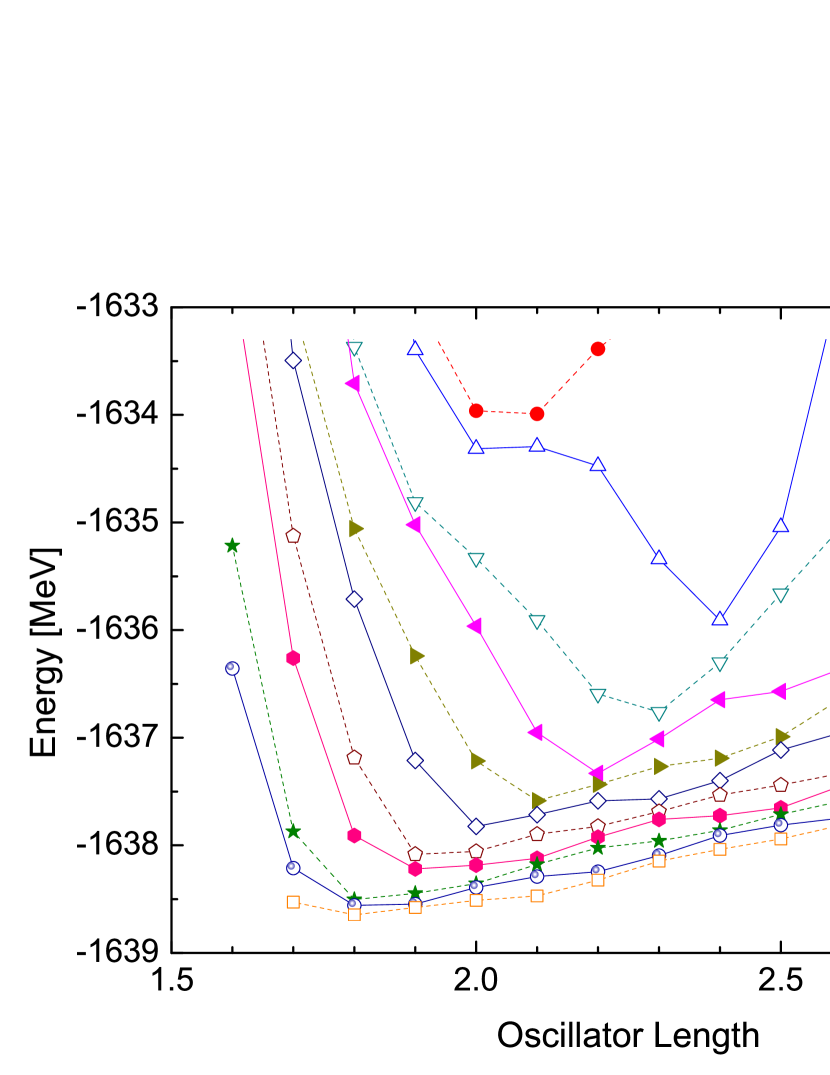
Figure 2: (color online) Convergence of the energy for the ground-state of ²⁰⁸Pb as function of the HO oscillator length $b=\sqrt{m\omega_{0}/\hbar}$ for various number of oscillator shells.

Dense Linear Algebra - When expressed in a single-particle basis, the density $\rho(x,x^{\prime})$ becomes an actual matrix $\rho_{ij}$ defined as

$$\rho_{ij}=\iint dxdx^{\prime}\phi_{j}^{*}(x^{\prime})\rho(x,x^{\prime})\phi_{i}(x).$$ (6)

A general two-body interaction becomes a rank-4 tensor $v_{abcd}$. The HF potential is obtained by taking a tensor contraction:

$$\Gamma_{ac}=\sum_{bd}v_{abcd}\rho_{db},$$ (7)

where the summation for each index extends over the size of the basis. Such tensor contractions must be performed at every iteration and represent an important bottleneck in the calculation. Indeed, for a heavy nucleus, the size of the HO basis for a precise calculation contains typically $N>20$ shells. In a Cartesian basis, this implies that each index $a,b,c,d$ is in fact a set of three numbers, $a\rightarrow\boldsymbol{n}_{a}\equiv(n_{x,a},n_{y,a},n_{z,a})$ with $n_{x,a}+n_{y,a}+n_{z,a}=N$. A naive implementation of Eq. (7) would therefore require a 12-nested loop to compute the entire matrix $\Gamma_{ac}$. Most problematic, in double-precision arithmetic the size of the complex tensor $v_{abcd}$ would be on the order of 80 TB after taking into account the anti-symmetry properties of $v_{abcd}$. Current implementations therefore do not store the matrix $v_{abcd}$ but compute it on the fly, adding to the computational overhead, and store the matrix $\Gamma_{ac}$ instead ($\sim$ 50 MB storage).

An alternative technique to compute $\Gamma_{ac}$, which avoids handling directly the tensor $v_{abcd}$ and is particularly efficient when the functional depends only on the local density matrix, relies on the fact that the functional dependence of $\Gamma$ on the density matrix $\rho$ is known. The HF potential for a local functional is simplified: $\Gamma[\rho(x,x^{\prime})]\rightarrow\Gamma[\rho(x)]$. The matrix $\Gamma_{ac}$ can then be computed by only one 3D integral:

$$\Gamma_{ac}=\int dx\phi_{j}^{*}(x)\Gamma[\rho(x)]\phi_{i}(x).$$ (8)

Such integrations can be performed exactly by quadrature formulas. The only time-consuming part of this method is to obtain an expression of $\rho(x)$ on the quadrature mesh, that is, $\rho(x_{k_{x}},y_{k_{y}},z_{k_{z}})$. One must compute

$$\rho(x_{k_{x}},y_{k_{y}},z_{k_{z}})=\sum_{\boldsymbol{m}\boldsymbol{n}}\sum_{\mu}V_{\boldsymbol{m}\mu}^{*}V_{\boldsymbol{n}\mu}\phi_{\boldsymbol{n}}^{*}(x_{k_{x}},y_{k_{y}},z_{k_{z}})\phi_{\boldsymbol{m}}(x_{k_{x}},y_{k_{y}},z_{k_{z}}).$$ (9)

This dense linear algebra requires at first sight 10-nested loops to build the entire representation of $\rho$ on the integration grid. Various numerical tricks can be used to reduce this number [8].

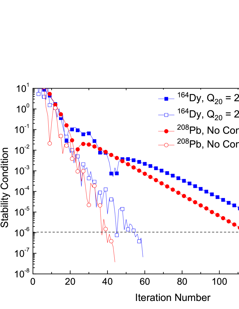
Figure 3: (color online) Convergence of the energy of two different nuclei with and without constraint on the quadrupole moment using standard linear mixing and the modified Broyden method [9].

Figure 4: (color online) Small-scale illustration of convergence failure. The figure shows a 2D cross-section of the potential energy landscape in ²⁴⁰Pu. Black points are calculated points; missing points did not converge.

Iterative Algorithms - The HFB equations are usually solved by iterations: starting at iteration 0 with an initial guess for, for example, the density matrix $\rho_{\text{in}}^{(0)}$ and pairing tensor $\kappa_{\text{in}}^{(0)}$, one constructs the HFB matrix $M^{(0)}$; diagonalizing it gives the eigenvectors at iteration 0, which are used to compute an updated version of the density matrix $\rho_{\text{out}}^{(0)}$ and pairing tensor $\kappa_{\text{out}}^{(0)}$; using these updates as input to iteration 1, one constructs the new HFB matrix $M^{(1)}$, diagonalizes it, and so forth, until convergence is met. Formally, this can be written as

$$\boldsymbol{V}_{\text{out}}^{(m)}=\boldsymbol{I}(\boldsymbol{V}_{\text{in}}^{(m)}).$$ (10)

The solution to the HFB equation satisfies: $\boldsymbol{V}=\boldsymbol{I}(\boldsymbol{V})$, or equivalently $\boldsymbol{F}(\boldsymbol{V})=\boldsymbol{V}-\boldsymbol{I}(\boldsymbol{V})=0$. This is a form of the fixed-point problem. Most DFT solvers iterate $\boldsymbol{V}$ either with a standard linear mixing,

$$\boldsymbol{V}_{\text{in}}^{(m+1)}=\alpha\boldsymbol{V}_{\text{out}}^{(m)}+(1-\alpha)\boldsymbol{V}_{\text{in}}^{(m)},$$ (11)

or a more elaborate mixing like the modified Broyden mixing [9]. The final number of iterations needed to reach convergence is extremely dependent on the type of calculation: ground-state properties of a spherical nucleus may take as little as 30 iterations, while the scission configuration in ²⁴⁰Pu may take as much as 5,000 iterations [10]. In addition, the iterative method often fails to converge, especially with large “exotic” constraints. Since the time of calculation is ultimately linearly proportional to the number of iterations, controlling the latter and ensuring a high convergence rate is critical for DFT applications.

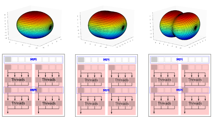
Figure 5: (color online) Hybrid MPI/OpenMP programming model for large-scale DFT applications: the process grid is decomposed in MPI communicators made of a few nodes (1 - 16), handling a given HFB calculation, with OpenMP threading within nodes.

3.2 Large-Scale Applications

In itself, one HFB calculation is almost always manageable on a standard computer. However, realistic applications always require the computation of a very large number of different configurations. The static description of nuclear fission is a good example: at least four deformation degrees of freedom are necessary—elongation, triaxiality, mirror symmetry, and neck size—just for calculations at zero temperature and zero angular momentum. A typical estimate for the number of points for each degree of freedom is $500\times 40\times 20\times 20=8.10^{6}$ points. At each point, one can estimate the error due to the truncation of the basis by repeating the same calculation with several different combinations of basis parameters: assuming 10 points per basis parameter, this adds a factor of 1,000. The typical size of the problem is therefore on the order of $10^{9}--10^{12}$ independent calculations, each taking on the order of a few days on a single core for high-precision results. This estimate applies to a single nucleus only.

Modern DFT solvers have therefore adopted a hybrid MPI/OpenMP programming model, illustrated in Fig. 5. Since a large number of HFB calculations is needed for any realistic problem, the process grid is decomposed into many small MPI communicators, each in charge of handling one HFB task, and possibly spanning multiple nodes. In order to accelerate dense linear algebra operations, OpenMP threading is used within a node. In many applications, only one MPI task per node is devoted to an HFB calculation. With existing solvers, the number of files needed to dump the output of the calculation grows as the number of HFB configurations handled: navigating this large mass of data and extracting the most relevant information pertaining to the problem at hand can be tricky. Some effort has therefore been put into the development of interfaces with advanced data mining software [11].

4 Recent Achievements

Collaborative efforts such as the SciDAC 2 UNEDF project have enabled ground-breaking optimizations of nuclear DFT solvers [12], which in turn have led to important discoveries in several areas of the physics of heavy nuclei. We highlight below two examples of recent work.

Figure 6: (color online) Differences between theoretical and experimental atomic masses for SLy4 (gray) and UNEDF1 (red) parametrization. Each line corresponds to an isotopic sequence. Adapted from [13].

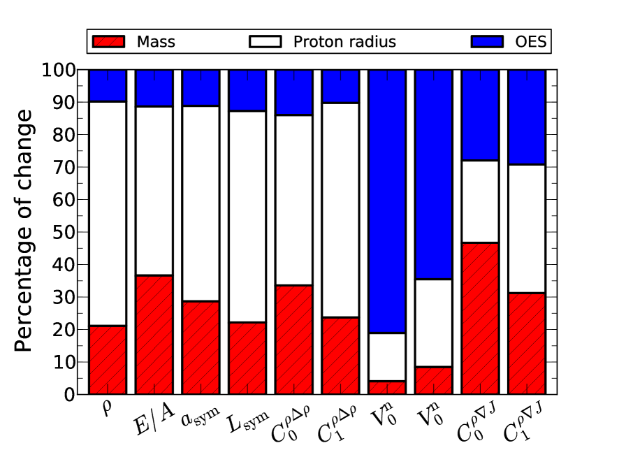
Figure 7: (color online) Sensitivity of the parameters of the Skyrme functional to various types of experimental data included in the optimization. Adapted from [13].

Optimization of Energy Functionals - The only input to nuclear DFT is the dozen or so low-energy constants characterizing the energy functionals. These parameters need to be carefully adjusted to experimental data. In the past, this procedure was usually carried out for specific systems such as infinite nuclear matter or doubly magic spherical nuclei, essentially because calculations are fast for those cases. However, most realistic nuclei are significantly different from such idealized systems, and it has been realized that many energy functionals suffer from systematic biases. The availability of heavily optimized DFT solvers together with leadership-class computers has allowed parameter optimization to be performed in realistic nuclei, that is, deformed nuclei with pairing. Moreover, statistical methods can now be applied at the solution to investigate the sensitivity of the solution to the experimental data, as well as built-in correlations between the parameters. Such modern methods have shed new light on the validity of current functionals and are now being applied to new generations of functionals [13].

Description of the Fission Process - The successful description of the fission process in the framework of DFT is a poster-child example of a large-scale computational problem involving nuclear DFT that could have tremendous applications for society. Most of the recent progress in the field has come from the computational side. In particular, the first systematic self-consistent survey of fission pathways with several shape degrees of freedom has been carried out in the region of the heaviest elements. Calculated lifetimes are in reasonable agreement with experiment; see Fig. 9 [14]. In parallel, preliminary studies of compound nucleus fission have shed new light on the probability of formation for superheavy elements in fusion reactions; see Fig. 9 [15, 16].

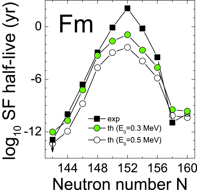
Figure 8: (color online) Theoretical and experimental fission half-lives of even-even Fermium isotopes.

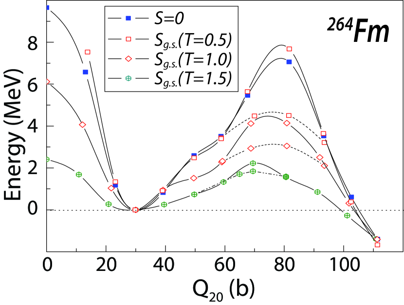
Figure 9: (color online) Symmetric isentropic fission pathways of ²⁶⁴Fm (energy normalized to the ground-state) including triaxial degrees of freedom (dashed lines).

5 Moving Forward

Computing Excited States - Most of the examples presented in this article correspond to the ground-state properties of nuclei. A significant challenge to DFT is its ability to also describe excited states. In the version of DFT that derives from a two-body effective interaction, indications are that a three-body force will have to be explicitly included. Doing so would enable to apply a well-established set of techniques such as projection and the generator coordinate method that can provide excited spectra. However, these methods will require yet another leap in the number of HFB points to be computed: for example, tensor contractions with a three-body force will increase from 12 to 18 the number of nested loops needed to compute the mean-field $\Gamma_{ac}$ in Cartesian coordinates.

Advanced Data Management - Currently, all DFT solvers have a rather simple I/O system, which essentially relies on native Fortran or C/C++ routines for disc access. Files are written on a per core basis: in large-scale applications, the number of files becomes huge and its management rather complex, and the scalability may degrade quickly as one hits the limits of the operating system; see Fig. 11. It seems therefore necessary to invest into more efficient I/O systems, possibly interfaced with professional database management and data-mining software. Indeed, a specific feature of DFT is that it produces a lot of data points that need to be analyzed in many different ways.

Real-time Simulation Steering - Current large-scale simulations are intrinsically static: given a set of input data shared among processes, each group of cores performs its task until completion. However, entire regions of potential energy surfaces irrelevant for physics applications cannot be detected until postanalysis is performed; calculations that failed could be converged with, for example, slightly different mixing parameters; model space dependence could be efficiently studied by optimizaton over the basis parameters, rather than meshing the parameter space. All these observations point to the need of dynamically steering the simulation based on a set of preliminary results. However, such a program can be viable only if the time of one HFB calculation can be reduced to at least less than 1 hour.

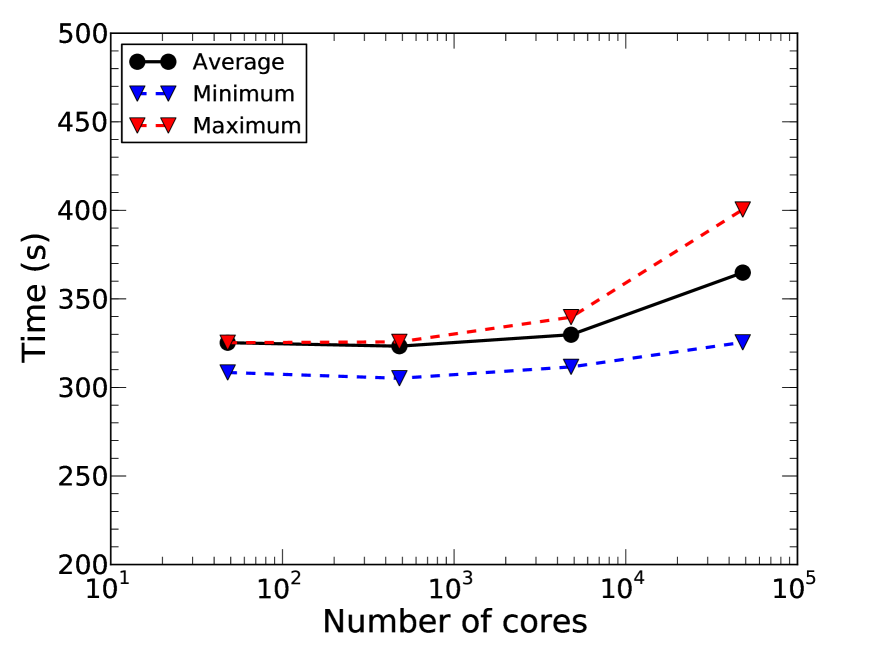
Figure 10: (color online) Scaling of the DFT solver HFODD for identical calculations run in parallel. Most of the load-imbalance and imperfect scaling comes from I/O. From [12].

Figure 11: (color online) Time of calculation for six HFB iterations depending on the ScaLAPACK diagonalization routine and the process grid (matrices of rank 2760).

Parallel Dense Linear Algebra Libraries - The reduction of the typical computation time below the 1-hour barrier is not possible without the development of highly optimized parallel dense linear algebra libraries. The current ScaLAPACK library provides a good starting point, but many routines do not reach the same level of performance as the original LAPACK versions. Currently, the gain is probably not sufficient for many practical application; see Fig. 11.

6 Conclusions

Nuclear DFT is the only theoretical framework that can be applied to all nuclei from the lightest to the heaviest, including stellar environments. While relatively mature, the theory has only recently started to benefit from the availability of leadership-class computers and advances in code development. Significant progress has been achieved, in particular in terms of parameter optimization and specific applications such as fission or large-scale surveys [17]. It is reasonable to anticipate that numerical uncertainties due to the truncation of the model space (HO basis) and the collective space (number of deformations) could be virtually eliminated in the near future, which would then open the door to high-precision nuclear simulations of importance to science and society. Such a promise, though, can be delivered only by the joint effort of both nuclear scientists and computer scientists. On the computational side, some of the key aspects are the parallelization of dense linear algebra operations, the development of real-time simulation steering tools, and the implementation of scalable I/O models and data management tools.

References

References

- [1] M. Bender, P.-H. Heenen, and P.-G. Reinhard, Rev. Mod. Phys. 75, 121 (2003).
- [2] J. Dobaczewski, M.V. Stoitsov, W. Nazarewicz, and P.-G. Reinhard, C 76, 054315 (2007).
- [3] T. Duguet and J. Sadoudi, J. Phys. G: Nucl. Part. Phys. 37 064009 (2010).
- [4] K. Bennaceur and J. Dobaczewski, Comput. Phys. Commun. 168, 96 (2005).
- [5] J. C. Pei, M. V. Stoitsov, G. I. Fann, W. Nazarewicz, N. Schunck, and F. R. Xu, Phys. Rev. C 78, 064306 (2008).
- [6] N. Nikolov, N. Schunck, W. Nazarewicz, M. Bender, and J. Pei, Phys. Rev. C 83, 034305 (2011).
- [7] G.I. Fann, J. Pei, R.J. Harrison, J. Jia, J. Hill, M. Ou, W. Nazarewicz, W. A. Shelton, and N. Schunck, J. Phys, Conference Series; 180 012080 (2009) Proc. SciDAC 2009 Conference, San Diego, CA.
- [8] J. Dobaczewski, W. Satuła, B.G. Carlsson, J. Engel, P. Olbratowski, P. Powałowski, M. Sadziak, J. Sarich, N. Schunck, A. Staszczak, M.V. Stoitsov, M. Zalewski, and H. Zduńczuk, Comput. Phys. Commun. 180, 2361 (2009).
- [9] A. Baran, A. Bulgac, M. McNeil Forbes, G. Hagen, W. Nazarewicz, N. Schunck, and M.V. Stoitsov, Phys. Rev. C 78, 014318 (2008).
- [10] W. Younes and D. Gogny, Phys. Rev. C 80, 054313 (2009).
- [11] http:massexplorer.org.
- [12] N. Schunck, J. Dobaczewski, J. McDonnell, W. Satuła, J.A. Sheikh, A. Staszczak, M. Stoitsov, P. Toivanen, arXiv:1103.1851 (2011).
- [13] M. Kortelainen, T. Lesinski, J. Moré, W. Nazarewicz, J. Sarich, N. Schunck, M.V. Stoitsov, and S. Wild, Phys. Rev. C 82, 024313 (2010).
- [14] A. Staszczak, A. Baran, J. Dobaczewski and W. Nazarewicz, Phys. Rev. C 80, 014309 (2009).
- [15] J.C. Pei, W. Nazarewicz, J.A. Sheikh, A.K. Kerman, Phys. Rev. Lett. 102, 192501 (2009).
- [16] J.A. Sheikh, W. Nazarewicz, J.C. Pei, Phys. Rev. C 80, 011302 (2009).
- [17] N. Schunck, J. Dobaczewski, J. Moré, J. McDonnell, W. Nazarewicz, J. Sarich, and M. V. Stoitsov, Phys. Rev. C 81, 024316 (2010).