1 Introduction

The Kolmogorov [1] and Kraichnan [2] theories of three- and two-dimensional Navier-Stokes turbulence have served as a benchmark in the understanding of fluid turbulence and as fundamental tests for the accuracy of simulations. The Boussinesq approximation of the compressible Navier-Stokes equations in a rotating frame give a fairly accurate description of the flow dynamics over much of the Earth’s oceans and atmosphere but are prohibitively expensive to simulate in detail over global scales. Guided by the success of the Kolmogorov/Kraichnan theories, it would be useful to develop a statistical phenomenology of the small scales of Boussinesq flows to gain an understanding of the physics, serve as benchmarks to test simulations, and offer parameterizations which could eventually be useful in practical modeling of geophysical flows. In addition to global energy, the inviscid Boussinesq equations conserve local potential vorticity (hereafter, PV) and global potential enstrophy, thus offering more complexity than incompressible Navier-Stokes dynamics. Charney [3] addressed one limiting case of the Boussinesq approximation, namely the quasi-geostrophic limit of strong rotation and strong stratification, and showed that the conservation of both energy and the quadratic potential enstrophy in such flows constrained energy to cascade to the large scales as in 2D turbulence [2].

Conservation of potential enstrophy is believed to play a fundamental role in the dynamics of the atmosphere and oceans [4]. Understanding its function in nonlinear scale interactions would appear to be essential for extending Kolmogorov’s theory to Boussinesq flows with rotation and stratification. Herring et al. [5] studied the cascade properties of potential enstrophy in turbulence simulations with a passive scalar in the absence of rotation and stratification. The authors concluded that because potential enstrophy in their simulation is not a quadratic, but a quartic invariant, the usual Kolmogorov-like arguments for a cascade and an inertial range do not apply. In fact, their potential enstrophy budget shows the direct action of viscous-diffusion terms at all scales, even in the limit of very small viscosity and diffusivity. Their figure 15 shows that potential enstrophy dissipation peaks at the largest scales (see also their figure 14 and the discussion on pp. 37 and 43). Thus, a pure inertial range of potential enstrophy flux is precluded because of contamination by dissipation at all scales. However for Boussinesq flows, with strong rotation and/or strong stratification, Kurien et al. [6] (hereafter, KSW06) derived analytically, starting from the evolution of the two-point correlation of potential vorticity, a flux law for potential enstrophy which is analogous to Kolmogorov’s 4/5-law for energy flux in 3D incompressible turbulence. The so-called 2/3-law of KSW06 implies that an inertial cascade of potential enstrophy can exist in three limiting cases: (i) strong rotation with moderate stratification (ii) moderate rotation with strong stratification and (iii) strong rotation and strong stratification. By “moderate” we mean that the rotation (stratification) frequency is of the same order as the non-linear turbulence frequency; whereas by “strong” we mean that the respective frequencies are much faster than the non-linear timescale. In the above three regimes, KSW06 showed that potential enstrophy, generally a quartic quantity, becomes quadratic which results in the localization of viscous-diffusion terms to the smallest scales, thus allowing for an inertial range of scales dominated by the flux of potential enstrophy. Furthermore, KSW06 suggested that in the absence of strong rotation and/or strong stratification, when potential enstrophy reverts to being quartic, viscous-diffusion effects may contaminate all scales, in agreement with the conclusions of [5].

The existence of an inertial cascade range for potential enstrophy is far from obvious and remains an unsettled issue. To date, there has been no empirical demonstration of KSW06’s results on the constant flux range of potential enstrophy in Boussinesq flows. In [7] a phenomenology and supporting data from Boussinesq simulations with equally strong (non-dimensional) rotation and stratification were presented to show that conservation of quadratic potential enstrophy could constrain the spectral distribution of energy in the large wavenumbers. In [8] the analysis and phenomenology of [7] was extended to include the two other limiting cases (i) and (ii) above, to show that indeed in all parameter regimes with linear PV, the downscale flux of (quadratic) potential enstrophy can constrain the scale-distribution of energy. While the two studies [7, 8] did not measure potential enstrophy flux, their numerical findings confirmed phenomenologically predicted scalings of the energy spectra assuming constant downscale fluxes of potential enstrophy. Motivated partially by those results, the present work uses data from [8] to directly measure the cascade of potential enstrophy for the first time.

Some previous studies have highlighted the interest in energy fluxes. The results from [9, 10] of purely stratified flow computed in small-aspect-ratio domains with forcing of the horizontal velocity only, did not show convincing constant energy fluxes (see figure 18 of [9] and figure 15 of [10] which plot energy flux on a log-log scale). On the other hand [11] provides evidence of scale-independent fluxes of kinetic and potential energy in purely stratified flow in unit aspect-ratio. It should be noted that these studies used forcing, stratification, and domain aspect-ratio different from ours. Furthermore, the simulations of [9, 10, 11] were not reported to be in the linear PV regime and, therefore, our results may not apply to their flows. Most importantly, none of these previous studies computed or analyzed the potential enstrophy flux, which constitutes an essential part of our work.

In this Letter, we present a very general framework for analyzing nonlinear scale interactions in Boussinesq flows. The coarse-graining approach we utilize allows for probing the dynamics simultaneously in space and in scale. Motivated by the work of [6, 7, 8], we then measure fluxes of energy and potential enstrophy across scales from simulations in three distinct limits of rotation and stratification. Our results show constant and positive fluxes of the two quadratic invariants, indicating simultaneous persistent downscale cascades of both quantities in all three cases. Our measurements of potential enstrophy flux are a novel contribution of this Letter and constitute the first empirical confirmation of analytical results by [6]. Furthermore, our evidence of a scale-independent energy flux is significant because it conveys that a cascade should persist to arbitrarily small scales at asymptotically high simulation resolutions.

2 Boussinesq dynamics

We study stably stratified Boussinesq flows in a rotating frame. The dynamics is described by momentum (1) and active scalar (2) equations:

$$\partial_{t}{\bf u}+({\bf u}{\mbox{\boldmath$\cdot$}}{\mbox{\boldmath$\nabla$}}){\bf u} = -{\mbox{\boldmath$\nabla$}}p-f\hat{{\bf z}}{\mbox{\boldmath$\times$}}{\bf u}-N\theta\hat{{\bf z}}+\nu\nabla^{2}{\bf u}+{\boldsymbol{\mathcal{F}}}^{u},$$ (1)

$$\partial_{t}\theta+({\bf u}{\mbox{\boldmath$\cdot$}}{\mbox{\boldmath$\nabla$}})\theta = Nu_{z}+\kappa\nabla^{2}\theta+{\mathcal{F}}^{\theta}.$$ (2)

Here, ${\bf u}$ is a solenoidal velocity field, ${\mbox{\boldmath$\nabla$}}{\mbox{\boldmath$\cdot$}}{\bf u}=0$, whose vertical component is $u_{z}$. The effective pressure is $p$, and ${\boldsymbol{\mathcal{F}}}^{u}$,${\mathcal{F}}^{\theta}$ are external forces. Gravity, $g$, is constant and in the $-\hat{{\bf z}}$ direction. Total density is given by $\rho_{T}({\bf x})=\rho_{0}-bz+\rho({\bf x})$, such that $|\rho({\bf x})|\ll|bz|$ and $|\rho({\bf x})|\ll\rho_{0}$, where $\rho_{0}$ is a constant background density, $b$ is constant and positive for stable stratification, and $\rho({\bf x})$ is the fluctuating density field with zero mean. The normalized density, $\theta({\bf x})=\sqrt{g/b\rho_{0}}\rho({\bf x})$, has units of velocity. For a constant rotation rate $\Omega$ about the z-axis, the Coriolis parameter is $f=2\Omega$. The Brunt-Väisälä frequency is $N=\sqrt{gb/\rho_{0}}$, kinematic viscosity is $\nu=\mu/\rho_{0}$, and mass diffusivity is $\kappa$. In this paper, we only study flows with Prandtl number $Pr=\nu/\kappa={\cal O}(1)$. Relevant non-dimensional parameters are Rossby number, $Ro=f_{nl}/f$, and Froude number, $Fr=f_{nl}/N$, where we define the characteristic non-linear frequency as $f_{nl}=(\epsilon_{f}k_{f}^{2})^{1/3}$, for a given energy injection rate $\epsilon_{f}$ at wavenumber $k_{f}$ (see [12, 6, 8]).

The dynamics of inviscid and unforced Boussinesq flows (such that $\nu=\kappa={\mathcal{F}}^{\theta}={\mathcal{F}}^{u}_{i}=0$) is constrained by the conservation of potential vorticity, $q({\bf x})=\frac{N}{b}{\mbox{\boldmath$\omega$}}_{a}{\mbox{\boldmath$\cdot$}}{\mbox{\boldmath$\nabla$}}\rho_{T}$, following material flow particles, $D_{t}q=\partial_{t}q+({\bf u}{\mbox{\boldmath$\cdot$}}{\mbox{\boldmath$\nabla$}})q=0$. Here, absolute vorticity is ${\mbox{\boldmath$\omega$}}_{a}={\mbox{\boldmath$\omega$}}+f\hat{{\bf z}}$ and local vorticity is ${\mbox{\boldmath$\omega$}}={\mbox{\boldmath$\nabla$}}{\mbox{\boldmath$\times$}}{\bf u}$. PV may be written in terms of $\omega$ and $\theta$ as

$$q({\bf x})=f\partial_{z}\theta-N{\mbox{\boldmath$\omega$}}{\mbox{\boldmath$\cdot$}}\hat{{\bf z}}+{\mbox{\boldmath$\omega$}}{\mbox{\boldmath$\cdot$}}{\mbox{\boldmath$\nabla$}}\theta-fN.$$ (3)

The first two terms are linear and dominate over the quadratic term, ${\mbox{\boldmath$\omega$}}{\mbox{\boldmath$\cdot$}}{\mbox{\boldmath$\nabla$}}\theta$, in the limit of large $f$ and/or large $N$. The constant part in (3) does not participate in the dynamics and can, therefore, be neglected [12].

In addition to conservation of PV, the flow is constrained by the global conservation of potential enstrophy, $Q=\frac{1}{2}q^{2}$, such that $\frac{d}{dt}\langle Q\rangle=0,$ where $\langle\dots\rangle=\frac{1}{V}\int_{V}d^{3}{\bf x}(\dots)$ is a space average. Another quadratic invariant of the inviscid dynamics is total mean energy, $E_{T}=\frac{1}{2}\langle|{\bf u}|^{2}+|\theta|^{2}\rangle$, such that $\frac{d}{dt}E_{T}=0.$

3 Numerical data

The Sandia-LANL DNS code was used to perform pseudo-spectral calculations of the Boussinesq equations (1)-(2) on grids of $640^{3}$ points in unit aspect-ratio domains. The time-stepping is 4th-order Runge-Kutta and the fastest linear wave frequencies are resolved with at least five timesteps per wave period. The diffusion of both momentum and density (scalar) is modeled by hyperviscosity of laplacian to the 8th-power. The coefficient of the hyperviscous diffusion term is chosen dynamically such that the energy in the largest wavenumber shell (smallest resolved scale) is dissipated at each time-step [13, 12]. This choice ensures that one does not have to guess the coefficient a priori and is a way to allow the flow itself to determine the magnitude of the diffusion. Hyperviscosity is a standard dissipation model that has long been used in studies of rotating and/or stratified flows [9, 10, 11, 12]. In principle, hyperviscosity can lead to thermalization and isotropy at the smallest scales [14], however our results on the inertial-range cascades are robust and unaffected by the small-scale dissipation model [15]. Stochastic forcing is incompressible and equipartitioned between the three velocity components and $\theta$. The forcing spectrum is peaked at $k_{f}=4\pm 1$, for large scale forcing. We use the two-thirds dealiasing rule. These data were reported in [7, 8], where further computational details may be found.

Run	resolution	$f~{}(Ro)$	$N~{}(Fr)$
Rs	$640^{3}$	$3000~{}(.002)$	$14~{}(.4)$
rS	$640^{3}$	$14~{}(.4)$	$3000~{}(.002)$
RS	$640^{3}$	$3000~{}(.002)$	$3000~{}(.002)$

Table 1: Parameters of the Boussinesq simulation data.

We analyze three sets of simulations corresponding to three extreme flow regimes summarized in Table 1. The first, Rs, is a flow under strong rotation and moderate stratification, $f/N\gg 1$. The second, rS, is a flow under moderate rotation but strong stratification, $f/N\ll 1$. The third, RS, is a flow under strong rotation and strong stratification such that $f=N$. Figure 1 shows that in all three cases, $\langle Q\rangle$ is well approximated by (one half) the square of the corresponding linear PV to within $3\%$ or better (see [6, 8]). Figure 1 is evidence that our simulations are in regimes of strong rotation and/or strong stratification. We analyze snapshots of the flow at late times when $\langle Q\rangle$ along with small-scale energy spectra (at wavenumbers $k\geq 6$) have reached a statistically steady state. The total energy, however, continues to grow due to an accumulation at the largest scales.

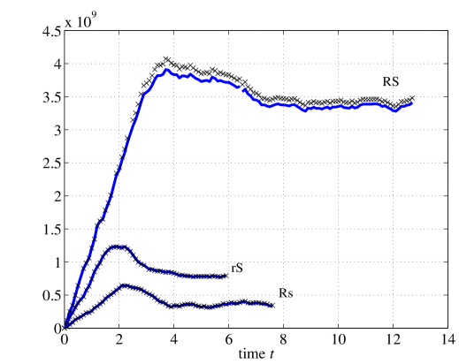
Figure 1: Time-series of mean potential enstrophy $\langle Q\rangle$ (solid line), and its quadratic part $\langle\widetilde{Q}\rangle$ (crosses). In run RS $\langle\widetilde{Q}\rangle=\big{\langle}\left[f\partial_{z}\theta-N{\mbox{\boldmath$\omega$}}{\mbox{\boldmath$\cdot$}}\hat{{\bf z}}\right]^{2}\big{\rangle}/2$; in run rS $\langle\widetilde{Q}\rangle=\big{\langle}\left[N{\mbox{\boldmath$\omega$}}{\mbox{\boldmath$\cdot$}}\hat{{\bf z}}\right]^{2}\big{\rangle}/2$; and in run Rs $\langle\widetilde{Q}\rangle=\big{\langle}\left[f\partial_{z}\theta\right]^{2}\big{\rangle}/2$. The plots show that $\langle Q\rangle$ reaches steady-state and that $\langle Q\rangle\simeq\langle\widetilde{Q}\rangle$ in all three regimes considered.

4 Analyzing the cascades by coarse-graining

Following [16, 17, 18, 19], we use a simple filtering technique common in the Large Eddy Simulation (LES) literature to resolve turbulent fields simultaneously in scale and in space. Other decompositions, such as wavelet analysis, also allow for the simultaneous space-scale resolution and may be used to analyze nonlinear scale interactions as well.

We define a coarse-grained or (low-pass) filtered field in $d$-dimensions as

$$\overline{\bf a}_{\ell}({\bf x})=\int d^{d}{\bf r}~{}G_{\ell}({\bf r}){\bf a}({\bf x}+{\bf r}),$$ (4)

where $G({\bf r})$ is a normalized convolution kernel, $\int d^{d}{\bf r}~{}G({\bf r})=1$. An example of such a kernel is the Gaussian function, $G(r)=\frac{1}{\sqrt{2\pi}}e^{-r^{2}/2}$. Its dilation $G_{\ell}({\bf r})\equiv\ell^{-d}G({\bf r}/\ell)$ in $d$-dimensions has its main support in a ball of radius $\ell$. Operation (4) may be interpreted as a local space average. In the rest of our Letter, we shall omit subscript $\ell$ whenever there is no ambiguity.

Applying the filtering operation (4) to the dynamics (1)-(2) yields coarse-grained equations that describe the evolution of $\overline{{\bf u}}_{\ell}({\bf x})$ and $\overline{\theta}_{\ell}({\bf x})$ at every point ${\bf x}$ in space and at any instant of time:

$$\partial_{t}\overline{\bf u}+(\overline{\bf u}{\mbox{\boldmath$\cdot$}}{\mbox{\boldmath$\nabla$}})\overline{\bf u} = -{\mbox{\boldmath$\nabla$}}\overline{p}-f\hat{{\bf z}}{\mbox{\boldmath$\times$}}\overline{\bf u}-N\overline{\theta}\hat{{\bf z}}$$ (5)

$$-{\mbox{\boldmath$\nabla$}}{\mbox{\boldmath$\cdot$}}\,\overline{\tau}({\bf u},{\bf u})+\nu\nabla^{2}\overline{\bf u}+\overline{{\boldsymbol{\mathcal{F}}}^{u}},$$

$$\partial_{t}\overline{\theta}+(\overline{\bf u}{\mbox{\boldmath$\cdot$}}{\mbox{\boldmath$\nabla$}})\overline{\theta} = N\,\overline{u}_{z}-{\mbox{\boldmath$\nabla$}}{\mbox{\boldmath$\cdot$}}\,\overline{\tau}({\bf u},\theta)$$ (6)

$$+\kappa\nabla^{2}\overline{\theta}+\overline{{\mathcal{F}}^{\theta}},$$

where subgrid stresses, $\overline{\tau}_{\ell}(f,g)\equiv\overline{fg}_{\ell}-\overline{f}_{\ell}~{}\overline{g}_{\ell}$, are “generalized 2nd-order moments” [17] accounting for the influence of eliminated fluctuations at scales $<\ell$.

The coarse-grained equations describe flow at scales $>\ell$, for arbitrary $\ell$. The approach, therefore, allows for the simultaneous resolution of dynamics both in scale and in space. Furthermore, the approach admits intuitive physical interpretation of various terms in the coarse-grained balance (5)-(6) which resemble the original governing eqs. (1)-(2), except for additional subgrid terms which quantify the nonlinear coupling between resolved and filtered scales. These subgrid terms depend inherently on the unresolved dynamics which has been filtered out. Traditional modeling efforts, such as in LES (see for example [20]), focus on devising closures for such terms which are plausible but whose regimes of applicability and validity are inevitably unknown. A key feature of the formalism employed here that distinguishes it from those modeling efforts is that it allows us to estimate the contribution of subgrid terms as a function of the resolution scale $\ell$ through exact mathematical analysis and direct numerical simulations (see for example [21, 22, 23, 24]). Our approach thus quantifies the coupling that exists between different scales and may be used to extract certain scale-invariant features in the dynamics.

4.1 Large-scale energy budget

From eqs. (5) and (6), it is straightforward to derive an energy budget for the large-scales, which reads

$$\partial_{t}\left(\frac{|\overline{\bf u}|^{2}}{2}+\frac{|\overline{\theta}|^{2}}{2}\right)+{\mbox{\boldmath$\nabla$}}{\mbox{\boldmath$\cdot$}}{\bf J}_{\ell} = -\Pi_{\ell}-\nu|{\mbox{\boldmath$\nabla$}}\overline{\bf u}|^{2}-\kappa|{\mbox{\boldmath$\nabla$}}\overline{\theta}|^{2}\hskip 17.07164pt$$

$$+\overline{\bf u}{\mbox{\boldmath$\cdot$}}\overline{{\boldsymbol{\mathcal{F}}}^{u}}+\overline{\theta}~{}\overline{{\mathcal{F}}^{\theta}}.$$

Here, $\nu|{\mbox{\boldmath$\nabla$}}\overline{\bf u}|^{2}+\kappa|{\mbox{\boldmath$\nabla$}}\overline{\theta}|^{2}$ is molecular dissipation acting on scales $>\ell$, and $\overline{\bf u}{\mbox{\boldmath$\cdot$}}\overline{{\boldsymbol{\mathcal{F}}}^{u}}+\overline{\theta}~{}\overline{{\mathcal{F}}^{\theta}}$ is energy injected due to external stirring. The term ${\bf J}_{\ell}({\bf x})$ represents space transport of large-scale energy whose complete expression is deferred to an Appendix below. Subgrid scale (SGS) flux, $\Pi_{\ell}({\bf x})$, accounts for the nonlinear transfer of energy from scales $>\ell$ to smaller scales:

$$\Pi_{\ell}({\bf x})=-\partial_{j}\overline{u}_{i}\overline{\tau}(u_{i},u_{j})-\partial_{j}\overline{\theta}~{}\overline{\tau}(\theta,u_{j}).$$ (8)

The SGS flux in (8) is work done by large-scale velocity and scalar gradients, ${\mbox{\boldmath$\nabla$}}\overline{\bf u}({\bf x})$ and ${\mbox{\boldmath$\nabla$}}\overline{\theta}({\bf x})$, against subgrid stresses. It acts as a sink in the large-scale budget (4.1) and accounts for the energy transferred across scale $\ell$ at any point ${\bf x}$ in the flow. Furthermore, $\Pi_{\ell}({\bf x})$ is Galilean invariant. Other definitions of a flux are possible, such as $\Pi_{\ell}({\bf x})=\overline{u}_{i}u_{j}\partial_{j}(u_{i}-\overline{u}_{i})$ (Eq. (2.52) in Frisch [25]), which differs from our definition (8) by a total gradient (disregarding the scalar part). However, these alternate definitions are not pointwise Galilean invariant, so the amount of energy cascading at any point ${\bf x}$ in the fluid according to such definitions would depend on the observer’s velocity.

Another physical requirement on the SGS flux $\Pi_{\ell}({\bf x})$ is that it should vanish in the absence of fluctuations at scales smaller than $\ell$ [21, 22]. For example, when $\ell=K^{-1}_{max}$, where $K_{max}$ is the maximum wavenumber in a pseudospectral simulation, there should be no cascade across $\ell$ simply because fluctuations at wavevectors $|{\bf k}|>K_{max}$ have zero amplitude. This is satisfied by our definition (8) identically at every point ${\bf x}$ in the flow. Alternate definitions such as $\Pi_{\ell}({\bf x})=\overline{u}_{i}u_{j}\partial_{j}u_{i}$ (eq. (6) in [26]) fail this pointwise requirement of a flux.

4.2 Large-scale $Q$ budget

Similar to the momentum, scalar, and energy equations (5)-(4.1), we can write down large-scale balances for PV and $Q$. The “bare” PV equation with diffusion and external forcing may be derived from eqs. (1) and (2) as

$$\partial_{t}q+({\bf u}{\mbox{\boldmath$\cdot$}}{\mbox{\boldmath$\nabla$}})q = \nu({\mbox{\boldmath$\nabla$}}\theta-N\hat{{\bf z}})\,{\mbox{\boldmath$\cdot$}}\nabla^{2}{\mbox{\boldmath$\omega$}}_{a}+\kappa{\mbox{\boldmath$\omega$}}_{a}{\mbox{\boldmath$\cdot$}}\nabla^{2}{\mbox{\boldmath$\nabla$}}\theta~{}~{}$$

$$+({\mbox{\boldmath$\nabla$}}\theta-N\hat{{\bf z}})\,{\mbox{\boldmath$\cdot$}}{{\boldsymbol{\mathcal{F}}}^{\omega}}+{\mbox{\boldmath$\omega$}}_{a}{\mbox{\boldmath$\cdot$}}{\mbox{\boldmath$\nabla$}}{{\mathcal{F}}^{\theta}},$$

where ${{\boldsymbol{\mathcal{F}}}^{\omega}}={\mbox{\boldmath$\nabla$}}{\mbox{\boldmath$\times$}}{{\boldsymbol{\mathcal{F}}}^{u}}$. Applying the filtering operation to (4.2) in the limit of strong rotation and/or stratification (limit of large $f$ and/or $N$ such that PV is linear, $q=f\partial_{z}\theta-N\omega_{z}$), yields the following balance for large-scale PV

$$\partial_{t}\overline{q}+(\overline{{\bf u}}{\mbox{\boldmath$\cdot$}}{\mbox{\boldmath$\nabla$}})\overline{q} = -{\mbox{\boldmath$\nabla$}}{\mbox{\boldmath$\cdot$}}\overline{\tau}(q,{\bf u})-\nu\,N\,\nabla^{2}\overline{\omega}_{z}+\kappa\,f\,\nabla^{2}\partial_{z}\overline{\theta}\hskip 5.69054pt$$ (10)

$$-N\,\overline{{\mathcal{F}}^{\omega}}_{z}+f\,\partial_{z}\overline{{\mathcal{F}}^{\theta}}.$$

Using (10), we can now write the large-scale potential enstrophy budget in the limit of linear PV,

$$\partial_{t}\frac{|\overline{q}|^{2}}{2}+{\mbox{\boldmath$\nabla$}}{\mbox{\boldmath$\cdot$}}{\bf J}^{Q}=-\Pi^{Q}-D^{Q}+\epsilon_{inj}^{Q},$$ (11)

where ${\bf J}^{Q}({\bf x})$ is space transport, $D^{Q}_{\ell}({\bf x})$ is dissipation due to viscosity and diffusivity acting directly on scales $>\ell$, and $\epsilon_{inj}^{Q}$ is the potential enstrophy injected due to external forcing. These terms are defined in [15]. $\Pi^{Q}_{\ell}({\bf x})$ is SGS flux of potential enstrophy,

$$\Pi^{Q}_{\ell}({\bf x})=-\partial_{j}\overline{q}~{}\overline{\tau}(q,u_{j}).$$ (12)

It is straightforward to verify that $\Pi^{Q}_{\ell}({\bf x})$ is Galilean invariant and vanishes in the absence of subgrid fluctuations.

5 Calculating fluxes using sharp spectral filter

We choose the so-called “sharp spectral filter” as our coarse-graining kernel in the definition of fluxes. We denote a field in a periodic domain $[0,1)^{3}$, coarse-grained with the spherically symmetric sharp-spectral filter to retain only Fourier modes $|{\bf k}|<K$, by

$${\bf a}^{<K}({\bf x})\equiv\sum_{|{\bf k}|\leq K}d{\bf k}~{}\hat{{\bf a}}({\bf k})e^{i2\pi{\bf k}\cdot{\bf x}}.$$ (13)

This is similar to $\overline{\bf a}_{\ell}({\bf x})$ with $\ell\sim K^{-1}$. We omit the factor $2\pi$ in reference to wavenumber in this Letter. While an isotropic filter such as (13) cannot distinguish between different directions, it does not average out anisotropy if present in a flow as will be clearly demonstrated in [15].

Using this filter, we can discern the amount of energy and potential enstrophy cascading across a certain wavenumber $K$. For example, to analyze the energy cascade, we can compute

$$\Pi_{K}({\bf x})=-\partial_{j}u_{i}^{<K}\tau^{<K}(u_{i},u_{j})-\partial_{j}\theta^{<K}\tau^{<K}(\theta,u_{j})$$ (14)

as a function of $K$. Here, $\tau^{<K}(f,g)=(fg)^{<K}-f^{<K}g^{<K}$. We can also analyze potential enstrophy cascade using

$$\Pi^{Q}_{K}({\bf x})=-\partial_{j}q^{<K}\tau^{<K}(q,u_{j}).$$ (15)

SGS energy flux (14) coincides with that used in [9, 10] only after space averaging. Yet, our quantity has the correct pointwise physical properties discussed above and, therefore, allows for studying spatial properties of the cascades.

6 Numerical Results

In this Letter, we restrict our numerical investigation to spatially averaged fluxes using the sharp spectral filter. Figure 2 shows that there is a positive and constant flux (y-axis shown on a linear scale to highlight true constancy) of total energy to small scales in all three cases of rotation and stratification. While all three cases show a clear downscale energy cascade, the RS case also has a negative flux over $K\leq 4$ possibly indicative of the expected inverse cascade present in such regime (e.g. [27, 28, 29]). We do not have the required scale-range in our simulations to say anything more definitive about the dynamics at scales larger than that of forcing.

We wish to emphasize the constancy of fluxes. A constant flux indicates a persistent non-linear transfer of energy to smaller scales, i.e. the flow is able to sustain a cascade to arbitrarily small scales, regardless of how small the viscous-diffusion parameters are. The term “cascade” necessitates a flux constant in wavenumber. It is certainly possible for non-linear interactions to yield a transient transfer to smaller scales but one which does not persist (decays to zero) and cannot carry the energy all the way to molecular scales. This is sometimes observed, for example, in 2D turbulence simulations and experiments (e.g. Figure 1 in [30]), where we know that a positive downscale flux of energy is only transient and cannot be constant (e.g. Figure 1 in [31]). Such distinction between transient and constant fluxes is imperative to modeling efforts. In the former case, there is no cascade or enhancement of dissipation due to turbulence whereas in the latter case, dissipation becomes independent of Reynolds number.

This issue is especially important when drawing conclusions from limited resolution simulations, true of most cases including ours. A constant flux indicates that dissipation should be independent of the simulation resolution. One may contend that a constant flux is just a consequence of a steady state and having forcing localized to the largest scales. However, it may very well be that the flow reaches steady state due to direct viscous dissipation acting on all scales as shown in [5] for potential enstrophy rather than a Kolmogorov-like inertial cascade.

Figure 2: Plots of total energy flux, $\langle\Pi_{K}\rangle$, from runs Rs (top), rS (middle), and RS (bottom). Dotted (blue) lines are fluxes taken from an instantaneous time snapshot. Solid (black) lines are averaged over time.

We also compute the potential enstrophy flux. Figure 3 shows that, in a manner similar to that of energy, there is a positive and constant flux of potential enstrophy in all three extreme cases. The plots in Figure 3 are the first measurements of potential enstrophy flux in rotating stratified Boussinesq flows and constitute one of the main results in this Letter. They can be regarded as the first empirical confirmation of analytical results in [6] which derived an exact law for potential enstrophy flux in physical space as a function of scale. Unlike for energy, $\langle\Pi^{Q}_{K}\rangle$ in Figure 3 for the RS case is not negative over $K\leq 4$.

Figure 3: Plots of potential enstrophy flux, $\langle\Pi^{Q}_{K}\rangle$, from runs Rs (top), rS (middle), and RS (bottom). Dotted (blue) lines are fluxes taken from an instantaneous time snapshot. Solid (black) lines are averaged over time.

Rotating and stratified flows are often said to be ‘two-dimensionalized’ in some sense, eliciting comparisons with two-dimensional turbulence and often justifying the study of the latter as a simplified paradigm for geophysical flows. Here we point out that the existence of a concurrent flux of both energy and potential enstrophy in rotating and stratified flow to smaller scales is in itself a marked departure of these flows from 2D turbulence. In the latter case, it is known (e.g. [2, 31]) that the two cascades cannot co-exist over the same scale-range since a forward cascade of enstrophy acts as a constraint leading to an inverse cascade of energy to larger scales.

In rotating and stratified flows, the velocity and scalar fields can be decomposed into the sum of a vortical component, which accounts for all the potential vorticity in the flow, and into a wave component, which has zero potential vorticity (e.g. [27, 12]). In the strongly rotating and strongly stratified regime, it is known (see [27, 28, 29]) that the vortical component of the flow is governed by quasigeostrophic dynamics, which is very similar to 2D turbulence [3]. In this regime, a forward energy cascade of the vortical component is suppressed due to the forward cascade of potential enstrophy. We verified (to appear in [15]) that this is indeed the case in our RS run, where the forward energy cascade (in Figure 2, bottom panel) is due to the wave component of the flow in agreement with [27]. However, the situation in the remaining two cases, runs Rs and rS, is markedly different from both 2D and quasigeostrophic dynamics as will be discussed in [15].

7 Conclusions

The two main results presented in this Letter are (i) energy and potential enstrophy budgets which resolve the dynamics simultaneously in space and in scale and (ii) concurrent and persistent cascades of energy and potential energy to small scales in three extreme cases of rotating and stratified Boussinesq flow simulations. The numerical results on constant fluxes of potential enstrophy constitute the first direct empirical evidence in support of analytical results by [6]. Our findings show a clear departure of the flows we study from 2-dimensional turbulence and should be incorporated in any phenomenological treatments of strongly rotating and/or stratified Boussinesq flows. In a longer forthcoming work [15], we shall refine our analysis to study anisotropy of these cascades, their pointwise and scale-locality properties, and quantify contributions from vortical and wave components.

Acknowledgements. This research used resources of the Argonne Leadership Computing Facility at Argonne National Laboratory, which is supported by the Office of Science of the US DOE under contract DE- AC02-06CH11357. HA acknowledges partial support from NSF grant PHY-0903872 during a visit to the Kavli Institute for Theoretical Physics. This research was performed under the auspices of the US DOE at LANL under Contract No. DE-AC52-06NA25396. HA was supported by the LANL/LDRD program and by the DOE ASCR program in Applied Mathematical Sciences. SK received partial funding from NSF program Collaborations in the Mathematical Geosciences: NSF CMG-1025188.

8 Appendix: Budgets

For the sake of completion, we write down the complete expression for the transport term in (4.1):

$$J_{j}({\bf x}) = \overline{u}_{j}\frac{|\overline{\bf u}|^{2}}{2}+\overline{u}_{i}~{}\overline{\tau}(u_{i},u_{j})-\nu\partial_{j}\frac{{|\overline{\bf u}|^{2}}}{2},$$

$$+ \overline{u}_{j}\frac{|\overline{\theta}|^{2}}{2}+\overline{\theta}~{}\overline{\tau}(\theta,u_{j})-\kappa\partial_{j}\frac{{|\overline{\theta}|^{2}}}{2}.$$

In large-scale potential enstrophy budget (11), ${\bf J}^{Q}({\bf x})$ is space transport, $D^{Q}_{\ell}({\bf x})$ is dissipation, and $\epsilon_{inj}^{Q}$ is the potential enstrophy injected due to external forcing. These are defined as

$$D^{Q}_{\ell}({\bf x}) = \nu N^{2}|{\mbox{\boldmath$\nabla$}}\overline{\omega}_{z}|^{2}+\kappa f^{2}|{\mbox{\boldmath$\nabla$}}\partial_{z}\overline{\theta}|^{2}-(\nu+\kappa)fN({\mbox{\boldmath$\nabla$}}\partial_{z}\overline{\theta}){\mbox{\boldmath$\cdot$}}{\mbox{\boldmath$\nabla$}}\overline{\omega}_{z}\hskip 19.91692pt$$ (17)

$$J^{Q}_{j}({\bf x}) = \overline{u}_{j}\frac{|\overline{q}|^{2}}{2}+\overline{q}~{}\overline{\tau}(u_{j},q)+\nu N~{}\overline{q}~{}\partial_{j}\overline{\omega}_{z}-\kappa f~{}\overline{q}~{}\partial_{j}\partial_{z}\overline{\theta},~{}~{}$$ (18)

$$\epsilon_{inj}^{Q}({\bf x}) = -N~{}\overline{q}~{}\overline{{\mathcal{F}}^{\omega}}_{z}+f~{}\overline{q}~{}\partial_{z}\overline{{\mathcal{F}}^{\theta}}$$ (19)

Note that while the first two dissipation terms in (17) are positive definite, the last term can be of either sign.

References

- [1] A. Kolmogorov. The local structure of turbulence in incompressible viscous fluid for very large Reynolds number. Dokl. Akad. Nauk SSSR, 30:9–13, 1941.
- [2] R. H. Kraichnan. Inertial Ranges in Two-Dimensional Turbulence. Phys. Fluids, 10:1417–1423, July 1967.
- [3] J. G. Charney. Geostrophic Turbulence. J. Atmos. Sci., 28:1087–1094, September 1971.
- [4] G. K. Vallis. Atmospheric and Oceanic Fluid Dynamics. Cambridge University Press, November 2006.
- [5] J. R. Herring, R. M. Kerr, and R. Rotunno. Ertel’s Potential Vorticity in Unstratified Turbulence. J. Atmos. Sc., 51:35–47, January 1994.
- [6] S. Kurien, L. Smith, and B. Wingate. On the two-point correlation of potential vorticity in rotating and stratified turbulence. J. Fluid Mech., 555:131–140, May 2006.
- [7] S. Kurien, B. Wingate, and M. A. Taylor. Anisotropic constraints on energy distribution in rotating and stratified turbulence. Europhys. Lett., 84:24003, October 2008.
- [8] S. Kurien. Scaling of high-wavenumber energy spectra in the unit aspect-ratio rotating Boussinesq system. unpublished, 2010. arXiv:1005.5366.
- [9] E. Lindborg. The energy cascade in a strongly stratified fluid. J. Fluid Mech., 550:207–242, March 2006.
- [10] G. Brethouwer, P. Billant, E. Lindborg, and J.-M. Chomaz. Scaling analysis and simulation of strongly stratified turbulent flows. J. Fluid Mech., 585:343–368, August 2007.
- [11] M. L. Waite. Stratified turbulence at the buoyancy scale. Phys. Fluids, 23:066602, 2011.
- [12] L. M. Smith and F. Waleffe. Generation of slow large scales in forced rotating stratified turbulence. J. Fluid Mech., 451:145–168, January 2002.
- [13] J. R. Chasnov. Similarity states of passive scalar transport in isotropic turbulence. Physics of Fluids, 6(2):1036 – 1051, FEB 1994.
- [14] Frisch, U. et al. Hyperviscosity, Galerkin Truncation, and Bottlenecks in Turbulence. Phys. Rev. Lett., 101(14):144501–+, October 2008.
- [15] H. Aluie and S. Kurien. Pointwise fluxes of energy and potential enstrophy, their anisotropy, and scale-locality in rotating stratified Boussinesq turbulence. In preparation, 2011.
- [16] A. Leonard. Energy Cascade in Large-Eddy Simulations of Turbulent Fluid Flows. Adv. Geophys., 18:A237, 1974.
- [17] M. Germano. Turbulence - The filtering approach. J. Fluid Mech., 238:325–336, 1992.
- [18] G. L. Eyink. Local energy flux and the refined similarity hypothesis. J. Stat. Phys., 78:335–351, 1995.
- [19] G. L. Eyink. Locality of turbulent cascades. Physica D, 207:91–116, 2005.
- [20] C. Meneveau and J. Katz. Scale-Invariance and Turbulence Models for Large-Eddy Simulation. Ann. Rev. Fluid Mech., 32:1–32, 2000.
- [21] G. Eyink and H. Aluie. Localness of energy cascade in hydrodynamic turbulence. I. Smooth coarse graining. Phys. Fluids, 21(11):115107, November 2009.
- [22] H. Aluie and G. Eyink. Localness of energy cascade in hydrodynamic turbulence. II. Sharp spectral filter. Phys. Fluids, 21(11):115108, November 2009.
- [23] H. Aluie and G. Eyink. Scale Locality of Magnetohydrodynamic Turbulence. Phys. Rev. Lett., 104(8):081101, February 2010.
- [24] H. Aluie. Compressible Turbulence: The Cascade and its Locality. Phys. Rev. Lett., 106(17):174502, April 2011.
- [25] U. Frisch. Turbulence. The legacy of A. N. Kolmogorov. Cambridge University Press, UK, 1995.
- [26] P. D. Mininni, A. Alexakis, and A. Pouquet. Nonlocal interactions in hydrodynamic turbulence at high Reynolds numbers: The slow emergence of scaling laws. Phys. Rev. E, 77(3):036306, 2008.
- [27] P. Bartello. Geostrophic Adjustment and Inverse Cascades in Rotating Stratified Turbulence. J. Atmos. Sci., 52:4410–4428, December 1995.
- [28] Babin, A. et al. On the Asymptotic Regimes and the Strongly Stratified Limit of Rotating Boussinesq Equations. Theor. Comput. Fluid Dyn., 9:223–251, 1997.
- [29] P. F. Embid and A. J. Majda. Low Froude number limiting dynamics for stably stratified flow with small or finite Rossby numbers. Geophys. Astrophys. Fluid Dyn., 87:1–50, 1998.
- [30] Chen, S. et al. Physical Mechanism of the Two-Dimensional Inverse Energy Cascade. Phys. Rev. Lett., 96(8):084502, February 2006.
- [31] G. Boffetta. Energy and enstrophy fluxes in the double cascade of two-dimensional turbulence. J. Fluid Mech., 589:253–260, 2007.