Assessment of synchrony in multiple neural spike trains using loglinear point process models

Abstract

Neural spike trains, which are sequences of very brief jumps in voltage across the cell membrane, were one of the motivating applications for the development of point process methodology. Early work required the assumption of stationarity, but contemporary experiments often use time-varying stimuli and produce time-varying neural responses. More recently, many statistical methods have been developed for nonstationary neural point process data. There has also been much interest in identifying synchrony, meaning events across two or more neurons that are nearly simultaneous at the time scale of the recordings. A natural statistical approach is to discretize time, using short time bins, and to introduce loglinear models for dependency among neurons, but previous use of loglinear modeling technology has assumed stationarity. We introduce a succinct yet powerful class of time-varying loglinear models by (a) allowing individual-neuron effects (main effects) to involve time-varying intensities; (b) also allowing the individual-neuron effects to involve autocovariation effects (history effects) due to past spiking, (c) assuming excess synchrony effects (interaction effects) do not depend on history, and (d) assuming all effects vary smoothly across time. Using data from the primary visual cortex of an anesthetized monkey, we give two examples in which the rate of synchronous spiking cannot be explained by stimulus-related changes in individual-neuron effects. In one example, the excess synchrony disappears when slow-wave “up” states are taken into account as history effects, while in the second example it does not. Standard point process theory explicitly rules out synchronous events. To justify our use of continuous-time methodology, we introduce a framework that incorporates synchronous events and provides continuous-time loglinear point process approximations to discrete-time loglinear models.

, and

1 Introduction

One of the most important techniques in learning about the functioning of the brain has involved examining neuronal activity in laboratory animals under varying experimental conditions. Neural information is represented and communicated through series of action potentials, or spike trains, and the central scientific issue in many studies concerns the physiological significance that should be attached to a particular neuron firing pattern in a particular part of the brain. In addition, a major relatively new effort in neurophysiology involves the use of multielectrode recording, in which responses from dozens of neurons are recorded simultaneously. Much current research focuses on the information that may be contained in the interactions among neurons. Of particular interest are spiking events that occur across neurons in close temporal proximity, within or near the typical one millisecond accuracy of the recording devices. In this paper we provide a point process framework for analyzing such nearly synchronous events.

The use of point processes to describe and analyze spike train data has been one of the major contributions of statistics to neuroscience. On the one hand, the observation that individual point processes may be considered, approximately, to be binary time series allows methods associated with generalized linear models to be applied [cf. Brillinger (1988, 1992)]. On the other hand, basic point process methodology coming from the continuous-time representation is important both conceptually and in deriving data-analytic techniques [e.g., the time-rescaling theorem may be used for goodness of fit and efficient spike train simulation; see Brown et al. (2001)]. The ability to go back and forth between continuous time, where neuroscience and statistical theory reside, and discrete time, where measurements are made and data are analyzed, is central to statistical analysis of spike trains. From the discrete-time perspective, when multiple spike trains are considered simultaneously it becomes natural to introduce loglinear models [cf. Martignon et al. (2000)] and a widely read and hotly debated report by Schneidman et al. (2006) examined the extent to which pairwise dependence among neurons can capture stimulus-related information. A fundamental limitation of much of the work in this direction, however, is its reliance on stationarity. The main purpose of the framework described below is to handle the nonstationarity inherent in stimulus-response experiments by introducing appropriate loglinear models while also allowing passage to a continuous-time limit. The methods laid out here are in the spirit of Ventura, Cai and Kass (2005), who proposed a bootstrap test of time-varying synchrony, but our methods are different in detail and our framework is much more general.

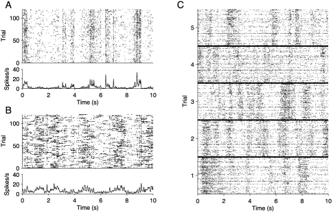
Figure 1: Neural spike train raster plots for repeated presentations of a drifting sine wave grating stimulus. (A) Single cell responses to 120 repeats of a 10 second movie. At the top is a raster corresponding to the spike times, and below is a peri-stimulus time histogram (PSTH) for the same data. Portions of the stimulus eliciting firing are apparent. (B) The same plots as in (A), for a different cell. (C) Population responses to the same stimulus, for 5 repeats. Each block, corresponding to a single trial, is the population raster for $\nu=128$ units. On each trial there are several dark bands, which constitute bursts of network activity sometimes called “up states.” Up state epochs vary across trials, indicating they are not locked to the stimulus.

Statistical modeling of point process data focuses on intensity functions, which represent the rate at which the events occur, and often involve covariates [cf. Brown et al. (2004), Kass, Ventura and Brown (2005), Paninski et al. (2009) and references therein]. A basic distinction is that of conditional versus marginal intensities: the conditional intensity determines the event rate for a given realization of the process, while the marginal intensity is the expectation of the conditional intensity across realizations. In neurophysiological experiments stimuli are often presented repeatedly across many trials, resulting in many replications of the multiple sequences of spike trains. This is the situation we concern ourselves with here, and it is illustrated in Figure 1, part A, where the responses of a single neuron for 120 trials are displayed: each line of the raster plot shows a single spike train, which is the neural response on a single trial. The experiment that generated these data is described in Section 1.1. The bottom panel in part A of Figure 1 displays a smoothed peristimulus time histogram (PSTH), which summarizes the trial-averaged response by pooling across trials. As we explain in greater detail in Section 1.2, scientific questions and statistical analyses may concern either within-trial responses (conditional intensities) or trial-averaged responses (marginal intensities).

A point process evolves in continuous time but, as we have noted, it is convenient for many statistical purposes to consider a discretized version. Decomposing time into bins of width $\delta$, we may define a binary time series to be 1 for every time bin in which an event occurs, and 0 for every bin in which an event does not occur. It is not hard to show that, under the usual regularity condition that events occur discretely (i.e., no two events occur at the same time), the likelihood function of the binary time series approximates the likelihood of the point process as $\delta\rightarrow 0$. For a pair of point processes, the discretized process is a time series of $2\times 2$ polytomous variables indicating, in each time bin, whether an event of the first process occurred, an event of the second process occurred, or both, or neither. This suggests analyzing nearly synchronous events based on a loglinear model with cell probabilities that vary across time. Intuitive as such procedures may be, their point process justification is subtle: the standard regularity condition forbids two processes having synchronous events, so it is not obvious how we might obtain convergence to a point process (as $\delta\rightarrow 0$) for discrete-process likelihoods that incorporate synchrony.

One way out of this impasse is to introduce a marked point process framework in which each event/mark could be of three distinct types: first process, second process, or both. The standard marked point process requires modification, however, because it fails to accommodate independence as a special case. Under independence, the discretized events for each process occur with probability of order $O(\delta)$, while the synchronous events occur with probability of order $O(\delta^{2})$ as $\delta\rightarrow 0$. We refer to this as a sparsity condition, and the generalization to multiple processes involves a hierarchical sparsity condition. Once we introduce a family of marked point processes indexed by $\delta$, we can guarantee hierarchical sparsity. Not only does this allow, as it must, the special case of independence models, but it also makes the conditional intensity for neuron $i$ depend only on the history for neuron $i$, asymptotically (as $\delta\rightarrow 0$). This in turn avoids confounding the dependence described by the loglinear model and greatly reduces the dimensionality of the problem. We require two very natural regularity conditions based on well-known neurophysiology: the existence of a refractory period, during which the neuron cannot spike again, and smoothness of the conditional intensity across time. It would be possible, and sometimes advantageous, instead to model dependence through the individual-neuron conditional intensity functions. The loglinear modeling approach used here avoids this step.

1.1 A motivating example

In a series of experiments performed by one of us (Kelly, together with Dr. Matthew Smith), visual images were displayed at resolution $1024\times 768$ pixels on a computer monitor, while the neural responses in the primary visual cortex of an anesthetized monkey were recorded. Each of 98 distinct images consisted of a sinusoidal grating that drifted in a particular direction for 300 milliseconds, and each was repeated 120 times. Each repetition of the complete sequence of stimuli lasted approximately 30 seconds. This kind of stimulus has been known to drive cells in the primary visual cortex since the Nobel prize-winning work of Hubel and Wiesel in the 1960s. With improved technology and advanced analytical strategies, much more precise descriptions of neural response are now possible. A small portion of the data from 5 repetitions of many stimuli is shown in part C of Figure 1.

The details of the experiment and recording technique are reported in Kelly et al. (2007). A total of 125 neural “units” were obtained, which included about 60 well-isolated individual neurons; the remainder were of undetermined origin (some mix of 1 or more neurons). The goal was to discover the interactions among these units in response to the stimuli. Each neuron will have its own consistent pattern of responses to stimuli, as illustrated in parts A and B of Figure 1. Synchronous spiking across neurons is relatively rare. However, in each of the 5 blocks within part C of Figure 1 (each block corresponding to a single trial) several dark bands of activity across most neurons may be seen during the trial. These bands correspond to what are often called network “up” states, and are often seen under anesthesia. For discussion and references see Kelly et al. (2010). It would be of interest to separate the effects of such network activity from other synchronous activity, especially stimulus-related synchronous activity. The framework in this paper provides a foundation for statistical methods that can solve such problems.

1.2 Overview of approach

We begin with some notation. Suppose we observe the activity of an ensemble of $\nu$ neurons labeled $1$ to $\nu$ over a time interval $[0,T)$, where $T>0$ is a constant. Let $N_{T}^{i}$ denote the total number of spikes produced by neuron $i$ on $[0,T)$ where $i=1,\ldots,\nu$. The resulting (stochastic) sequence of spike times is written as $0\leq s_{1}^{i}<\cdots<s^{i}_{N^{i}_{T}}<T$. For the moment we focus on the case $\nu=3$, but other values of $\nu$ are of interest and with contemporary recording technology $\nu\approx 100$ is not uncommon, as in the experiment in Section 1.1. Let $\delta>0$ be a constant such that $T$ is a multiple of $\delta$ (for simplicity). We divide the time interval into bins of width $\delta$. Define $X^{i}(t)=1$ if neuron $i$ has a spike in the time bin $[t,t+\delta)$ and $0$ otherwise. Because of the existence of a refractory period for each neuron, there can be at most 1 spike in $[t,t+\delta)$ from the same neuron if $\delta$ is sufficiently small. Then writing

$$P^{1,2,3}_{a,b,c}(t)=P\bigl{(}X^{1}(t)=a,X^{2}(t)=b,X^{3}(t)=c\bigr{)}\qquad\forall a,b,c\in\{0,1\},$$

the data would involve spike counts across trials [e.g., the number of trials on which $(X^{1}(t),$ $X^{2}(t),X^{3}(t))=(1,1,1)$]. The obvious statistical tool for analyzing spiking dependence is loglinear modeling and associated methodology.

Three complications make the problem challenging, at least in principle. First, there is nonstationarity: the probabilities vary across time. The data thus form a sequence of $2^{\nu}$ contingency tables. Second, absent from the above notation is a possible dependence on spiking history. Such dependence is the rule rather than the exception. Let $\bar{\mathcal{H}}^{i}_{t}$ denote the set of values of $X^{i}(s)$, where $s<t$, and $s,t$ are multiples of $\delta$. Thus, $\bar{\mathcal{H}}_{t}=(\bar{\mathcal{H}}^{1}_{t},\ldots,\bar{\mathcal{H}}^{\nu}_{t})$ is the history of the binned spike train up to time $t$. We may wish to consider conditional probabilities such as

$$P_{a,b,c}^{1,2,3}(t|\bar{\mathcal{H}}_{t})=P\bigl{(}X^{1}(t)=a,X^{2}(t)=b,X^{3}(t)=c|\bar{\mathcal{H}}_{t}\bigr{)}$$

for $a,b,c\in\{0,1\}$. Third, there is the possibility of precisely timed lagged dependence (or time-delayed synchrony): for example, we may want to consider the probability

$$P_{1,1,1}^{1,2,3}(s,t,u)=P\bigl{(}X^{1}(s)=1,X^{2}(t)=1,X^{3}(u)=1\bigr{)},$$ (1)

where $s,t,u$ may be distinct. Similarly, we might consider the conditional probability

$$P^{1,2,3}_{1,1,1}(s,t,u|\bar{\mathcal{H}}_{s}^{1},\bar{\mathcal{H}}_{t}^{2},\bar{\mathcal{H}}_{u}^{3})=P\bigl{(}X^{1}(s)=1,X^{2}(t)=1,X^{3}(u)=1|\bar{\mathcal{H}}_{s}^{1},\bar{\mathcal{H}}_{t}^{2},\bar{\mathcal{H}}_{u}^{3}\bigr{)}.$$

In principle, we would want to consider all possible combinations of lags. Even for $\nu=3$ neurons, but especially as we contemplate $\nu\gg 3$, strong restrictions must be imposed in order to have any hope of estimating all these probabilities from relatively sparse data in a small number of repeated trials. To reduce model dimensionality, we suggest four seemingly reasonable tactics: (i) considering models with only low-order interactions, (ii) assuming the probabilities $P^{1,2,3}_{a,b,c}(t)$ or $P_{a,b,c}^{1,2,3}(t|\bar{\mathcal{H}}_{t})$ vary smoothly across time $t$, (iii) restricting history effects to those that modify a neuron’s spiking behavior based on its own past spiking, and then (iv) applying analogues to standard loglinear model methodology. Combining these, we obtain tractable models for multiple binary time series to which standard methodology, such as maximum likelihood and smoothing, may be applied. In modeling synchronous spiking events as loglinear time series, however, it would be highly desirable to have a continuous-time representation, where binning becomes an acknowledged approximation. We therefore also provide a theoretical point process foundation for the discrete multivariate methods proposed here.

It is important to distinguish the probabilities $P_{a,b,c}^{1,2,3}(t)$ and $P_{a,b,c}^{1,2,3}(t|\bar{\mathcal{H}}_{t})$. The former are trial-averaged or marginal probabilities, while the latter are within-trial or conditional probabilities. Both might be of interest but they quantify different things. As an extreme example suppose, as sometimes is observed, each of two neurons has highly rhythmic spiking at an approximately constant phase relationship with an oscillatory potential produced by some large network of cells. Marginally these neurons will show strongly dependent spiking. On the other hand, after taking account of the oscillatory rhythm by conditioning on each neuron’s spiking history and/or a suitable within-trial time-varying covariate, that dependence may vanish. Such a finding would be informative, as it would clearly indicate the nature of the dependence between the neurons. In Section 3 we give a less dramatic but similar example taken from the data described in Section 1.1.

We treat marginal and conditional analyses separately. Our use of two distinct frameworks is a consequence of the way time resolution will affect continuous-time approximations. We might begin by imagining the situation in which event times could be determined with infinite precision. In this case it is natural to assume, as is common in the point process literature, that no two processes have simultaneous events. As we indicate, this conception may be applied to marginal analysis. However, the event times are necessarily recorded to fixed accuracy, which becomes the minimal value of $\delta$, and $\delta$ may be sufficiently large that simultaneous events become a practical possibility. Many recording devices, for example, store neural spike event times with an accuracy of 1 millisecond. Furthermore, the time scale of physiological synchrony—the proximity of spike events thought to be physiologically meaningful—is often considered to be on the order of $\delta=5$ milliseconds [cf. Grün, Diesmann and Aertsen (2002a, 2002b) and Grün (2009)]. For within-trial analyses of synchrony, the theoretical conception of simultaneous (or synchronous) spikes across multiple trials therefore becomes important and leads us to the formalism detailed below. The framework we consider here provides one way of capturing the notion that events within $\delta$ milliseconds of each other are essentially synchronous.

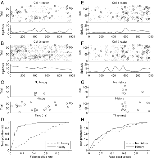
Figure 2: Synchronous spike analysis for two pairs of neurons. Results for one pair shown on left, in parts (A)–(D) and for the other pair on the right in parts (E)–(H). Part (A) Response of a cell to repetitions of a 1 second drifting grating stimulus. The raster plot is shown above and the smoothed PSTH below. Part (B) Response from a second cell, as in (A). In both (A) and (B), spikes that are synchronous between the pair are circled. Part (C) Correct joint spike predictions from model, shown as circles [as in parts (A) and (B)], when false positive rate is set at 10%. In top plot the joint spikes are from the history-independent model, as in (13), while in the bottom plot they are as in (16), including the network covariate in the history term. Part (D) ROC curves for the models in part (C). Parts (E), (F), (G) and (H) are similar to Parts (A), (B), (C) and (D) but for the second pair of neurons.

The rest of this article is organized as follows. Section 2 presents the methodology in three subsections: Sections 2.1 and 2.2 introduce marginal and conditional methods in the simplest case, while Section 2.3 discusses the use of loglinear models and associated methodology for analyzing spiking dependence. In Section 3 we illustrate the methodology by returning to the example of Section 1.1. The main purpose of our approach is to allow covariates to take account of such things as the irregular network rhythm displayed in Figure 1, so that synchrony can be understood as either related to the network effects or unrelated. Figure 2 displays synchronous spiking events for two different pairs of neurons, together with accompanying fits from continuous-time loglinear models. For both pairs the independence model fails to account for synchronous spiking. However, for one pair the apparent excess synchrony disappears when history effects are included in the loglinear model, while in the other pair they do not, leading to the conclusion that in the second case the excess synchrony must have some other source. Theory is presented in Sections 4–6. We add some discussion in Section 7. All proofs in this article are deferred to the Appendix.

2 Methodology

In this section we present our continuous-time loglinear modeling methodology. We begin with the simplest case of $\nu=2$ neurons, presenting the main ideas in Sections 2.1 and 2.2 for the marginal and conditional cases, respectively, in terms of the probabilities $P^{1}_{a}(t)=P(X^{1}(t)=a)$, $P^{1,2}_{a,b}(t)=P(X^{1}(t)=a,X^{2}(t)=b)$, etc., for all $a,b\in\{0,1\}$. We show how we wish to pass to the continuous-time limit, thereby introducing point process technology and making sense of continuous-time smoothing, which is an essential feature of our approach. In Section 2.3 we reformulate using loglinear models, and then give continuous-time loglinear models for $\nu=3$. Our analyses in Section 3 are confined to $\nu=2$ and $\nu=3$ because of the paucity of higher-order synchronous spikes in our data. Our explicit models for $\nu=3$ should make clear how higher-order models are created. We give general recursive formulas in Sections 5 and 6.

2.1 Marginal methods for $\nu=2$

The null hypothesis

$$H_{0}\dvtx P^{1,2}_{1,1}(t)=P_{1}^{1}(t)P^{2}_{1}(t)\qquad\forall t\in{\mathcal{T}}=\{0,\delta,2\delta,\ldots,T-\delta\}$$ (2)

is a statement that both neurons spike in the interval $[t,t+\delta)$, on the average, at the rate determined by independence. Defining $\zeta(t)$ by

$$P^{1,2}_{1,1}(t)=P^{1}_{1}(t)P^{2}_{1}(t)\zeta(t)\qquad\forall t\in{\mathcal{T}},$$ (3)

we may rewrite (2) as

$$H_{0}\dvtx\zeta(t)=1\qquad\forall t\in{\mathcal{T}}.$$ (4)

As in Ventura, Cai and Kass (2005), to assess $H_{0}$, the general strategy we follow is to (i) smooth the observed-frequency estimates of $P^{1}_{1}(t)$, $P^{2}_{1}(t)$ and $P^{1,2}_{1,1}(t)$ across time $t$, and then (ii) form a suitable test statistic and compute a $p$-value using a bootstrap procedure. We may deal with time-lagged hypotheses similarly, for example, for a lag $h>0$, we write

$$P^{1,2}_{1,1}(t,t+\delta h) = P\bigl{(}X^{1}(t)=1,X^{2}(t+\delta h)=1\bigr{)}$$

$$= P^{1}_{1}(t)P^{2}_{1}(t+\delta h)\zeta(t,t+\delta h),$$

then smooth the observed-frequency estimates for $P^{1,2}_{1,1}(t,t+\delta h)$ as a function of $t$, form an analogous test statistic and find a $p$-value.

To formalize this approach, we consider counting processes $N^{i}_{t}$ corresponding to the point processes $s_{1}^{i},s_{2}^{i},\ldots,s^{i}_{N^{i}_{t}}$, $i=1,2$ (as in Section 1.2 with $\nu=2$). Under regularity conditions, the following limits exist:

$$\lambda^{i}(t) = \lim_{\delta\rightarrow 0}\delta^{-1}P\bigl{(}N^{i}_{t+\delta}-N^{i}_{t}=1\bigr{)},$$

$$\lambda^{1,2}(t) = \lim_{\delta\rightarrow 0}\delta^{-2}P\bigl{(}(N^{1}_{t+\delta}-N^{1}_{t})(N^{2}_{t+\delta}-N^{2}_{t})=1\bigr{)},$$ (6)

$$\xi(t) = \lim_{\delta\rightarrow 0}\zeta(t).$$

Consequently, for small $\delta$, we have

$$P^{i}_{1}(t)\approx\lambda^{i}(t)\delta,\qquad P^{1,2}_{1,1}(t)\approx\lambda^{1,2}(t)\delta^{2}.$$

The smoothing of the observed-frequency estimates for $P_{1,1}^{1,2}(t)$ may be understood as producing an estimate $\hat{\lambda}^{1,2}(t)$ for $\lambda^{1,2}(t)$. The null hypothesis in (2) becomes, in the limit as $\delta\rightarrow 0$,

$$H_{0}\dvtx\lambda^{1,2}(t)=\lambda^{1}(t)\lambda^{2}(t)\qquad\forall t\in[0,T),$$

or, equivalently,

$$H_{0}:\xi(t)=1\qquad\forall t\in[0,T).$$ (7)

The lag $h$ case is treated similarly. Under mild conditions, Theorems 1 and 2 of Section 5 show that the above heuristic arguments hold for a continuous-time regular marked point process. This in turn gives a rigorous asymptotic justification (as $\delta\rightarrow 0$) for estimation and testing procedures such as those in steps (i) and (ii) mentioned above, following (4), and illustrated in Section 3.

2.2 Conditional methods for $\nu=2$

To deal with history effects, equation (3) is replaced with

$$P^{1,2}_{1,1}(t|\bar{\mathcal{H}}_{t})=P^{1}_{1}(t|\bar{\mathcal{H}}^{1}_{t})P^{2}_{1}(t|\bar{\mathcal{H}}^{2}_{t})\zeta(t)\qquad\forall t\in{\mathcal{T}},$$ (8)

where $\bar{\mathcal{H}}^{i}_{t}$, $i=1,2$, are, as in Section 1, the binned spiking histories of neurons 1 and 2, respectively, on the interval $[0,t)$. Analogous to (4), the null hypothesis is

$$H_{0}\dvtx\zeta(t)=1\qquad\forall t\in{\mathcal{T}}.$$

We note that there are two substantial simplifications in (8). First, $P^{i}_{1}(t|\bar{\mathcal{H}}_{t})=P^{i}_{1}(t|\bar{\mathcal{H}}^{i}_{t})$, which says that neuron $i$’s own history $\bar{\mathcal{H}}^{i}_{t}$ is relevant in modifying its spiking probability (but not the other neuron’s history). Second, $\zeta(t)$ does not depend on the spiking history $\bar{\mathcal{H}}_{t}$. This is important for what it claims about the physiology, for the way it simplifies statistical analysis, and for the constraint it places on the point process framework. Physiologically, it decomposes excess spiking into history-related effects and stimulus-related effects, which allows the kind of interpretation alluded to in Section 1 and presented in our data analysis in Section 3. Statistically, it improves power because tests of $H_{0}$ effectively pool information across trials, thereby increasing the effective sample size.

Consider counting processes $N^{i}_{t}$, $i=1,2$, as in Section 2.1. Under regularity conditions, the following limits exist for $t\in[0,T)$:

$$\lambda^{i}(t|{\mathcal{H}}^{i}_{t}) = \lim_{\delta\rightarrow 0}\delta^{-1}P(N^{i}_{t+\delta}-N^{i}_{t}=1|\bar{\mathcal{H}}_{t}^{i}),\qquad i=1,2,$$

$$\lambda^{1,2}(t|{\mathcal{H}}_{t}) = \lim_{\delta\rightarrow 0}\delta^{-2}P\bigl{(}(N^{1}_{t+\delta}-N^{1}_{t})(N^{2}_{t+\delta}-N^{2}_{t})=1|\bar{\mathcal{H}}_{t}\bigr{)},$$ (9)

$$\xi(t) = \lim_{\delta\rightarrow 0}\zeta(t),$$

where ${\mathcal{H}}_{t}=\lim_{\delta\rightarrow 0}\bar{\mathcal{H}}_{t}$ and ${\mathcal{H}}_{t}^{i}=\lim_{\delta\rightarrow 0}\bar{\mathcal{H}}_{t}^{i},i=1,2$. For sufficiently small $\delta$, we have

$$\hskip 25.0ptP^{i}_{1}(t|\bar{\mathcal{H}}^{i}_{t})\approx\lambda^{i}(t|{\mathcal{H}}^{i}_{t})\delta,\qquad i=1,2,\quad\mbox{and}\quad P^{1,2}_{1,1}(t|\bar{\mathcal{H}}_{t})\approx\lambda^{1,2}(t|{\mathcal{H}}_{t})\delta^{2}$$ (10)

for all $t\in{\mathcal{T}}$. Again following Ventura, Cai and Kass (2005), we may smooth the observed-frequency estimates of $P^{1,2}_{1,1}(t|\bar{\mathcal{H}}_{t})$ to produce an estimate of $\lambda^{1,2}(t|{\mathcal{H}}_{t})$, and smooth the observed-frequency estimates of $P^{i}_{1}(t|\bar{\mathcal{H}}^{i}_{t})$ to produce estimates of $\lambda^{i}(t|{\mathcal{H}}_{t}^{i})$, $i=1,2$. Letting $\delta\rightarrow 0$ in (8), we obtain

$$\lambda^{1,2}(t|{\mathcal{H}}_{t})=\xi(t)\lambda^{1}(t|{\mathcal{H}}_{t}^{1})\lambda^{2}(t|{\mathcal{H}}_{t}^{2})\qquad\forall t\in[0,T).$$ (11)

Consequently, for sufficiently small $\delta$, a conditional test of $H_{0}\dvtx\zeta(t)=1$ for all $t$ becomes a test of the null hypothesis $H_{0}\dvtx\lambda^{1,2}(t|{\mathcal{H}}_{t})=\lambda^{1}(t|{\mathcal{H}}_{t}^{1})\lambda^{2}(t|{\mathcal{H}}_{t}^{2})$ for all $t$ or, equivalently, in this conditional case we have the same null hypothetical statement as (7).

In attempting to make equation (2.2) rigorous, a difficulty arises: for a regular marked point process, the function $\xi$ need not be independent of the spiking history. This would create a fundamental mismatch between the discrete data-analytical method and its continuous-time limit. The key to avoiding this problem is to enforce the sparsity condition (10). Specifically, the probabilities $P^{i}_{1}(t|\bar{\mathcal{H}}^{i}_{t})$ are of order $O(\delta)$, while the probabilities $P^{1,2}_{1,1}(t|\bar{\mathcal{H}}_{t})$ are of order $O(\delta^{2})$. This also allows independence models within the marked point process framework. Section 6 proposes a class of marked point process models indexed by $\delta$ and provides results that validate the heuristics above.

2.3 Loglinear models

We now reformulate in terms of loglinear models the procedures sketched in Sections 2.1 and 2.2 for $\nu=2$ neurons, and then indicate the way generalizations proceed when $\nu\geq 3$.

In the marginal case of Section 2.1, it is convenient to define

$$\tilde{P}^{1,2}_{0,0}(t) = 1,$$

$$\tilde{P}^{1,2}_{1,0}(t) = P^{1}_{1}(t),$$

$$\tilde{P}^{1,2}_{0,1}(t) = P^{2}_{1}(t),$$

$$\tilde{P}^{1,2}_{1,1}(t) = P^{1,2}_{1,1}(t)\qquad\forall t\in{\mathcal{T}}.$$

Equation (3) implies that

$$\log[\tilde{P}^{1,2}_{a,b}(t)]=a\log[P^{1}_{1}(t)]+b\log[P^{2}_{1}(t)]+ab\log[\zeta(t)]$$ (12)

for all $a,b\in\{0,1\}$ and $t\in{\mathcal{T}}$ and in the continuous-time limit, using (2.1), we write

$$\log\lambda^{1,2}(t)=\log\lambda^{1}(t)+\log\lambda^{2}(t)+\log[\xi(t)]$$ (13)

for $t\in[0,T)$. The null hypothesis may then be written as

$$H_{0}\dvtx\log[\xi(t)]=0\qquad\forall t\in[0,T).$$ (14)

In the conditional case of Section 2.2, we similarly define

$$\tilde{P}^{1,2}_{0,0}(t|\bar{\mathcal{H}}_{t}) = 1,$$

$$\tilde{P}^{1,2}_{1,0}(t|\bar{\mathcal{H}}_{t}) = P^{1}_{1}(t|\bar{\mathcal{H}}_{t}),$$

$$\tilde{P}^{1,2}_{0,1}(t|\bar{\mathcal{H}}_{t}) = P^{2}_{1}(t|\bar{\mathcal{H}}_{t}),$$

$$\tilde{P}^{1,2}_{1,1}(t|\bar{\mathcal{H}}_{t}) = P^{1,2}_{1,1}(t|\bar{\mathcal{H}}_{t})\qquad\forall t\in{\mathcal{T}},$$

we may rewrite (8) as the loglinear model

$$\log[\tilde{P}^{1,2}_{a,b}(t|\bar{\mathcal{H}}_{t})]=a\log[P^{1}_{1}(t|\bar{\mathcal{H}}_{t}^{1})]+b\log[P^{2}_{1}(t|\bar{\mathcal{H}}_{t}^{2})]+ab\log[\zeta(t)]$$ (15)

for all $a,b\in\{0,1\}$ and $t\in{\mathcal{T}}$ and in the continuous-time limit we rewrite (11) in the form

$$\log\lambda^{1,2}(t|{\mathcal{H}}_{t})=\log\lambda^{1}(t|{\mathcal{H}}^{1}_{t})+\log\lambda^{2}(t|{\mathcal{H}}^{2}_{t})+\log[\xi(t)]$$ (16)

for $t\in[0,T)$. The null hypothesis may again be written as in (14).

Rewriting the model in loglinear forms (12), (13), (15) and (16) allows us to generalize to $\nu\geq 3$ neurons. For example, with the obvious extensions of the previous definitions, for $\nu=3$ neurons the two-way interaction model in the continuous-time marginal case becomes

$$\hskip 25.0pt\log[\tilde{P}^{1,2,3}_{a,b,c}(t)] = \log[P^{1}_{1}(t)]+\log[P^{2}_{1}(t)]+\log[P^{3}_{1}(t)]$$

$${}+ab\log\bigl{[}\zeta_{\{1,2\}}(t)\bigr{]}+ac\log\bigl{[}\zeta_{\{1,3\}}(t)\bigr{]}+bc\log\bigl{[}\zeta_{\{2,3\}}(t)\bigr{]}$$

for all $a,b,c\in\{0,1\}$ and $t\in{\mathcal{T}}$, and

$$\log[\lambda^{1,2,3}(t)] = \log[\lambda^{1}(t)]+\log[\lambda^{2}(t)]+\log[\lambda^{3}(t)]$$

$${}+\log\bigl{[}\xi_{\{1,2\}}(t)\bigr{]}+\log\bigl{[}\xi_{\{1,3\}}(t)\bigr{]}+\log\bigl{[}\xi_{\{2,3\}}(t)\bigr{]}$$

for all $t\in(0,T]$. The general form of (2.3) is given by equation (5.1) in Section 5. In the conditional case, the two-way interaction model becomes

$$\hskip 23.0pt\log[\tilde{P}^{1,2,3}_{a,b,c}(t|\bar{\mathcal{H}}_{t})] = a\log[P^{1}_{1}(t|\bar{\mathcal{H}}_{t})]+b\log[P^{2}_{1}(t|\bar{\mathcal{H}}_{t})]+c\log[P^{3}_{1}(t|\bar{\mathcal{H}}_{t})]$$

$${}+ab\log\bigl{[}\zeta_{\{1,2\}}(t)\bigr{]}+ac\log\bigl{[}\zeta_{\{1,3\}}(t)\bigr{]}+bc\log\bigl{[}\zeta_{\{2,3\}}(t)\bigr{]}$$

for all $a,b,c\in\{0,1\}$ and $t\in{\mathcal{T}}$ and in continuous time,

$$\log[\lambda^{1,2,3}(t|{\mathcal{H}}_{t})] = \log[\lambda^{1}(t|{\mathcal{H}}_{t})]+\log[\lambda^{2}(t|{\mathcal{H}}_{t})]+\log[\lambda^{3}(t|{\mathcal{H}}_{t})]$$

$${}+\log\bigl{[}\xi_{\{1,2\}}(t)\bigr{]}+\log\bigl{[}\xi_{\{1,3\}}(t)\bigr{]}+\log\bigl{[}\xi_{\{2,3\}}(t)\bigr{]}$$

for all $t\in(0,T]$. In either the marginal or conditional case, the null hypothesis of independence may be written as

$$H_{0}\dvtx\log\bigl{[}\xi_{\{i,j\}}(t)\bigr{]}=0\qquad\forall t\in(0,T],1\leq i<j\leq 3.$$ (19)

On the other hand, we could include the additional term $abc\log[\xi_{\{1,2,3\}}(t)]$ and use the null hypothesis of no three-way interaction

$$H_{0}\dvtx\log\bigl{[}\xi_{\{1,2,3\}}(t)\bigr{]}=0\qquad\forall t\in(0,T].$$ (20)

These loglinear models offer a simple and powerful way to study dependence among neurons when spiking history is taken into account. They have an important dimensionality reduction property in that the higher-order terms are asymptotically independent of history. In practice, this provides a huge advantage: the synchronous spikes are relatively rare; in assessing excess synchronous spiking with this model, the data may be pooled over different histories, leading to a much larger effective sample size. The general conditional model in equation (6.1) retains this structure. An additional feature of these loglinear models is that time-varying covariates may be included without introducing new complications. In Section 3 we use a covariate to characterize the network up states, which are visible in part C of Figure 1, simply by including it in calculating each of the individual-neuron conditional intensities $\lambda^{1}(t|{\mathcal{H}}^{1}_{t})$ and $\lambda^{2}(t|{\mathcal{H}}^{2}_{t})$ in (16).

Sometimes, as in the data we analyze here, the synchronous events are too sparse to allow estimation of time-varying excess synchrony and we must assume it to be constant, $\zeta(t)=\zeta$ for all $t$. Thus, for $\nu=2$, the models of (12) or (15) take simplified forms in which $\zeta(t)$ is replaced by the constant $\zeta$ and we would use different test statistics to test the null hypothesis $H_{0}\dvtx\zeta=1$. To distinguish the marginal and conditional cases, we replace $\zeta(t)$ by $\zeta_{H}$ in (15) and then also write $H_{0}\dvtx\zeta_{H}=1$. Moving to continuous time, which is simpler computationally, we write $\xi(t)=\xi$, estimate $\xi$ and $\xi_{H}$, and test $H_{0}\dvtx\xi=1$ and $H_{0}\dvtx\xi_{H}=1$. Specifically, we apply the loglinear models (12), (13), (15) and (16) in two steps. First, we smooth the respective PSTHs to produce smoothed curves $\hat{\lambda}^{i}(t)$, as in parts A and B of Figure 1. Second, ignoring estimation uncertainty and taking $\lambda^{i}(t)=\hat{\lambda}^{i}(t)$, we estimate the constant $\zeta$. Using the point process representation of joint spiking (justified by the results in Sections 5 and 6), we may then write

$$\log L(\xi)=-\int\lambda(t)\,dt+\sum\log\lambda(t_{i}),$$

where the sum is over the joint spike times $t_{i}$ and $\lambda(t)$ is replaced by the right-hand side of (13), in the marginal case, or (16), in the conditional case. It is easy to maximize the likelihood $L(\xi)$ analytically: setting the left-hand side to $\ell(\xi)$, in the marginal case we have

$$\ell^{\prime}(\xi)=-\int\lambda^{1}(t)\lambda^{2}(t)\,dt+\frac{N}{\xi},$$

where $N$ is the number of joint (synchronous) spikes (the number of terms in the sum), while in the conditional case we have the analogous formula

$$\ell^{\prime}(\xi_{H})=-\int\lambda^{1}(t|{\mathcal{H}}_{t}^{1})\lambda^{2}(t|{\mathcal{H}}_{t}^{2})\,dt+\frac{N}{\xi_{H}}$$

and setting to 0 and solving gives

$$\hat{\xi}=\frac{N}{\int\lambda^{1}(t)\lambda^{2}(t)\,dt}$$ (21)

and

$$\hat{\xi}_{H}=\frac{N}{\int\lambda^{1}(t|{\mathcal{H}}_{t}^{1})\lambda^{2}(t|{\mathcal{H}}_{t}^{2})\,dt},$$ (22)

which, in both cases, is the ratio of the number of observed joint spikes to the number expected under independence.

We apply (21) and (22) in Section 3. To test $H_{0}\dvtx\xi=1$ and $H_{0}\dvtx\xi_{H}=1$, we use a bootstrap procedure in which we generate spike trains under the relevant null-hypothetical model. This is carried out in discrete time, and requires all 4 cell probabilities $\tilde{P}^{1,2}_{a,b}(t)$ or $\tilde{P}^{1,2}_{a,b}(t|\bar{\mathcal{H}}_{t})$ at every time $t\in{\mathcal{T}}$. These are easily obtained by subtraction using $P^{1}_{1}(t)=\lambda^{1}(t)\delta$, $P^{2}_{1}(t)=\lambda^{2}(t)\delta$, and $\hat{\zeta}=\hat{\xi}$ or, in the conditional case, $P^{1}_{1}(t|\bar{\mathcal{H}}_{t}^{1})=\lambda^{1}(t|{\mathcal{H}}^{1}_{t})\delta$, $P^{2}_{1}(t|\bar{\mathcal{H}}_{t}^{2})=\lambda^{2}(t|{\mathcal{H}}^{2}_{t})\delta$, and $\hat{\zeta}_{H}=\hat{\xi}_{H}$. As we said above, $\lambda^{i}(t)=\hat{\lambda}^{i}(t)$ is obtained from the preliminary step of smoothing the PSTH. Similarly, the conditional intensities $\lambda^{i}(t|{\mathcal{H}}^{i}_{t})=\hat{\lambda}^{i}(t|{\mathcal{H}}^{i}_{t})$ are obtained from smooth history-dependent intensity models such as those discussed in Kass, Ventura and Brown (2005). In the analyses reported here we have used fixed-knot splines to describe variation across time $t$.

In the case of 3 or more neurons the analogous estimates and cell probabilities must, in general, be obtained by a version of iterative proportional fitting. For $\nu=3$, to test the null hypothesis (20), we follow the steps leading to (21) and (22). Under the assumption of constant $\zeta_{123}$, we obtain

$$\hat{\xi}_{123}=\frac{N}{\int\lambda^{1}(t)\lambda^{2}(t)\lambda^{3}(t)\xi_{12}(t)\xi_{13}(t)\xi_{23}(t)\,dt}$$ (23)

and

$$\hat{\xi}_{123,H}=\frac{N}{\int\lambda^{1}(t|{\mathcal{H}}_{t}^{1})\lambda^{2}(t|{\mathcal{H}}_{t}^{2})\lambda^{3}(t|{\mathcal{H}}_{t}^{3})\xi_{12,H}(t)\xi_{13,H}(t)\xi_{23,H}(t)\,dt}.$$ (24)

In Section 3 we fit (2.3) and report a bootstrap test of the hypothesis (20) using the test statistic $\hat{\xi}_{123}$ in (23).

3 Data analysis

We applied the methods of Section 2.3 to a subset of the data described in Section 1.1 and present the results here. We plan to report a more comprehensive analysis elsewhere.

We took $\delta=5$ milliseconds (ms), which is a commonly-used window width in studies of synchronous spiking. Raster plots of spike trains across repeated trials from a pair of neurons are shown in Parts A and B of Figure 2, with synchronous events indicated by circles. Below each raster plot is a smoothed PSTH, that is, the two plots show smoothed estimates $\hat{\lambda}^{1}(t)$ and $\hat{\lambda}^{2}(t)$ of $\lambda^{1}(t)$ and $\lambda^{2}(t)$ in (2.1), the units being spikes per second. Smoothing was performed by fitting a generalized additive model using cubic splines with knots spaced 100 ms apart. Specifically, we applied Poisson regression to the count data resulting from pooling the binary spike indicators across trials: for each time bin the count was the number of trials on which a spike occurred. To test $H_{0}$ under the model in (13), we applied (21) to find $\log\hat{\xi}$. We then computed a parametric bootstrap standard error of $\log\hat{\xi}$ by generating pseudo-data from model (13) assuming $H_{0}\dvtx\log\xi=0$. We generated 1000 such trials, giving 1000 pseudo-data values of $\log\hat{\xi}$, and computed the standard deviation of those values as a standard error, to obtain an observed $z$-ratio test statistic of 3.03 ($p=0.0012$ according to asymptotic normality).

The highly significant $z$ ratio shows that there is excess sychronous spiking beyond what would be expected from the varying firing rates of the two neurons under independence. However, it does not address the source of the excess synchronous spiking. The excess synchronous spiking could depend on the stimulus or, alternatively, it might be due to the slow waves of population activity evident in part (C) of Figure 1, the time of which vary from trial to trial and therefore do not depend on the stimulus. To examine the latter possibility, we applied a within-trial loglinear model as in (16) except that we incorporated into the history effect not only the history of each neuron but also a covariate representing the population effect. Specifically, for neuron $i$ ($i=1,2$) we used the same generalized additive model as before, but with two additional variables. The first was a variable that, for each time bin, was equal to the number of neuron $i$ spikes that had occurred in the previous 100 ms. The second was a variable that, for each time bin, was equal to the number of spikes that occurred in the previous 100 ms across the whole population of neurons, other than neurons 1 and 2. We thereby obtained fitted estimates $\hat{\lambda}^{1}(t|{\mathcal{H}}^{1}_{t})$ and $\hat{\lambda}^{2}(t|{\mathcal{H}}^{2}_{t})$ of $\lambda^{1}(t|{\mathcal{H}}^{1}_{t})$ and $\lambda^{2}(t|{\mathcal{H}}^{2}_{t})$. Note that the fits for the independence model, defined by applying (7) to (11), now vary from trial to trial due to the history effects. Applying (22), we found $\log\hat{\xi}_{H}$, and then again computed a bootstrap standard error of $\log\hat{\xi}_{H}$ by creating 1000 trials of pseudo-data, giving $\log\hat{\xi}_{H}=0.06\pm 0.15$, for a $z$-ratio of $0.39$, which is clearly not significant.

Raster plots for a different pair of neurons are shown in parts (E) and (F) of Figure 2. The same procedures were applied to this pair. Here, the $z$-ratio for testing $H_{0}$ under the marginal model was 3.77 ($p<0.0001$), while that for testing $H_{0}$ under the conditional model remained highly significant at 3.57 ($p=0.0002$) with $\log\hat{\xi}_{H}=0.82\pm 0.23$. In other words, using the loglinear model methodology, we have discovered two pairs of V1 neurons with quite different behavior. For the first pair, synchrony can be explained entirely by network effects, while for the second pair it can not; this suggests that, instead, for the second pair, some of the excess synchrony may be stimulus-related.

We also compared the marginal and conditional models (13) and (16) using ROC curves. Specifically, for the binary joint spiking data we used each model to predict a spike whenever the intensity was larger than a given constant: for the marginal case whenever $\log\lambda^{1,2}(t)>c_{\mathrm{marginal}}$, and for the conditional case whenever $\log\lambda^{1,2}(t|{\mathcal{H}}_{t})>c_{\mathrm{conditional}}$. The choice of constants $c_{\mathrm{marginal}}$ and $c_{\mathrm{conditional}}$ reflect trade-offs between false positive and true positive rates (analogous to type I error and power) and as we vary the constants, the plot of true vs. false positive rates forms the ROC curve. To determine the true and false positive rates, we performed ten-fold cross-validation, repeatedly fitting from 90% of the trials and predicting from the remaining 10% of the trials. The two resulting ROC curves are shown in part D of Figure 2, labeled as “no history” and “history,” respectively. To be clear, in the two cases we included the terms corresponding, respectively, to $\xi$ and $\xi_{H},$ and in the history case we included both the auto-history and the network history variables specified above. The ROC curve for the conditional model strongly dominates that for the marginal model, indicating far better predictive power. In part C of Figure 2 we display the true positive joint spike predictions when the false-positive rate was held at 10%. These correctly-predicted joint spikes may be compared to the complete set displayed in parts A and B of the figure. The top display in part C, labeled “no history,” shows that only a few joint spikes were correctly predicted by the marginal model, while the large majority were correctly predicted by the conditional model. Furthermore, the correctly predicted joint spikes are spread fairly evenly across time. In contrast, the ROC curves for the second pair of neurons, shown in part (G) of Figure 2, are close to each other: inclusion of the history effects (which were statistically significant) did not greatly improve predictive power. In (G), the correctly predicted synchronous spikes are clustered in time, with the main cluster occurring near a peak in the individual-neuron firing-rate functions shown in the two smoothed PSTHs in parts (E) and (F).

Taking all of the results together, our analysis suggests that the first pair of neurons produced excess synchronous spikes solely in conjunction with network effects, which are unrelated to the stimulus, while for the second pair of neurons some of the excess synchronous spikes occurred separately from the network activity and were, instead, stimulus-related.

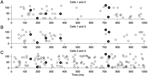
Figure 3: Plots of synchronous spiking events for 3 neurons. Each of the three plots displays all joint spikes (as circles) for a particular pair of neurons. The dark circles in each plot indicate the 3-way joint spikes.

We also tried to assess whether 2-way interactions were sufficient to explain observed 3-way events by fitting the no-3-way interaction model given by (2.3), and then testing the null hypothesis in (20). We did this for a particular set of 3 neurons, whose joint spikes are displayed in Figure 3. The method is analogous to that carried out above for pairs of neurons, in the sense that the test statistic was $\hat{\xi}_{123}$ given by (23) and a parametric bootstrap procedure, based on the fit of (2.3), was used to compute an approximate $p$-value. Fitting of (2.3) required an iterative proportional fitting procedure, which we will describe in detail elsewhere. We obtained $p=0.16$, indicating no significant 3-way interaction. In other words, for these three neurons, 2-way excess joint spiking appears able to explain the occurrence of the 3-way joint spikes. However, as may be seen in Figure 3, there are very few 3-way spikes in the data. We mention this issue again in our discussion.

4 A marked point process framework

In this section a class of marked point processes for modeling neural spike trains is briefly surveyed. These models take into account the possibility of two or more neurons firing in synchrony (i.e., at the same time). Consider an ensemble of $\nu$ neurons labeled $1$ to $\nu$. For $T>0$, let $N_{T}$ denote the total number of spikes produced by this ensemble on the time interval $[0,T)$ and let $0\leq s_{1}<\cdots<s_{N_{T}}<T$ denote the specific spike times. For each $j=1,\ldots,N_{T}$, we write $(s_{j},(i_{1},\ldots,i_{k}))$ to denote the event that a spike was fired (synchronously) at time $s_{j}$ by (and only by) the $i_{1}$, $\ldots$, $i_{k}$ neurons. We observe that

$${\mathcal{H}}_{T}=\{(s_{1},\kappa_{1}),\ldots,(s_{N_{T}},\kappa_{N_{T}})\dvtx\kappa_{j}\in{\mathcal{K}},j=1,\ldots,N_{T}\}$$ (25)

forms a marked point process on the interval $[0,T)$ with ${\mathcal{K}}$ as the mark space satisfying

$${\mathcal{K}}\subseteq\{(i_{1},\ldots,i_{k})\dvtx 1\leq i_{1}<\cdots<i_{k}\leq\nu,k=1,\ldots,\nu\}.$$

We follow Daley and Vere-Jones (2002), page 249, and define the conditional intensity function of ${\mathcal{H}}_{T}$ as

$$\lambda(t,\kappa|{\mathcal{H}}_{t})$$

$$\qquad=\lambda(t,\kappa|\{(s_{1},\kappa_{1}),\ldots,(s_{N_{t}},\kappa_{N_{t}})\})$$

$$\qquad=\cases{h_{1}(t)f_{1}(\kappa|t)\qquad\forall 0\leq t\leq s_{1},\cr h_{i}(t|(s_{1},\kappa_{1}),\ldots,(s_{i-1},\kappa_{i-1}))f_{i}(\kappa|t;(s_{1},\kappa_{1}),\ldots,(s_{i-1},\kappa_{i-1}))\cr\qquad\forall s_{i-1}<t\leq s_{i},i=2,\ldots,N_{T},\cr h_{N_{T}+1}(t|(\!s_{1},\kappa_{1}\!),\ldots,(s_{N_{t}},\kappa_{N_{T}}\!)\!)f_{N_{T}+1}(\kappa|t;(s_{1},\kappa_{1}\!),\ldots,(s_{N_{T}},\kappa_{N_{T}}\!)\!)\cr\qquad\forall s_{N_{T}}<t<T,}$$

where $h_{1}(\cdot)$ is the hazard function for the location of the first spike $s_{1}$, $h_{2}(\cdot|(s_{1},\kappa_{1}))$ the hazard function for the location of the second spike $s_{2}$ conditioned by $(s_{1},\kappa_{1})$, and so on, while $f_{1}(\cdot|t)$ is the conditional probability mass function of $\kappa_{1}$ given $s_{1}=t$, and so on. It is also convenient to write $\lambda(t,\kappa|\varnothing)=\lambda(t,\kappa|{\mathcal{H}}_{t})$ for all $t<s_{1}$. The following proposition and its proof can be found in Daley and Vere-Jones (2002), page 251.

Proposition 1

Let ${\mathcal{H}}_{T}$ be as in (25). Then the density of ${\mathcal{H}}_{T}$ is given by

$$p_{\lambda}({\mathcal{H}}_{T}) = p_{\lambda}(\{(s_{1},\kappa_{1}),\ldots,(s_{N_{T}},\kappa_{N_{T}})\})$$

$$= \Biggl{[}\prod_{i=1}^{N_{T}}\lambda(s_{i},\kappa_{i}|{\mathcal{H}}_{s_{i}})\Biggr{]}\exp\biggl{[}-\sum_{\kappa\in{\mathcal{K}}}\int_{0}^{T}\lambda(t,\kappa|{\mathcal{H}}_{t})\,dt\biggr{]}.$$

5 Theoretical results: Marginal methods

In this section we (i) provide a justification of the limiting statements in (2.1) and (ii) generalize to higher-order models. We also note that lagged dependence can be accommodated within our framework, treating the case $\nu=2$.

5.1 Regular marked point process and loglinear modeling

In this subsection we prove that the heuristic arguments of Section 2 for marginal methods hold under mild conditions. Consider $\nu\geq 1$ neurons labeled $1$ to $\nu$. For $T>0$, let $N_{T}$ denote the total number of spikes produced by these $\nu$ neurons on the time interval $[0,T)$ and let $0\leq s_{1}<\cdots<s_{N_{T}}<T$ denote the specific spike times. For each $j=1,\ldots,N_{T}$, we write $(s_{j},(i_{j}))$ to represent the event that a spike was fired at time $s_{j}$ by neuron $i_{j}$ where $i_{j}\in\{1,\ldots,\nu\}$. We observe from Section 4 that

$${\mathcal{H}}_{T}=\{(s_{1},(i_{1})),\ldots,(s_{N_{T}},(i_{N_{T}}))\}$$

forms a marked point process on the interval $[0,T)$ with mark space ${\mathcal{K}}=\{(1),\ldots,(\nu)\}$. Following the notation of Section 4, let $\lambda(t,(i)|{\mathcal{H}}_{t})$ denote the conditional intensity function of the point process ${\mathcal{H}}_{T}$. We assume that the following two conditions hold:

Condition (I). There exists a strictly positive refractory period for each neuron in that there exists a constant $\theta>0$ such that $\lambda(t,(i)|{\mathcal{H}}_{t})=0$ if there exists some $(s_{,}(i))\in{\mathcal{H}}_{t}$ such that $t-s\leq\theta,i\in\{1,\ldots,\nu\}$.

Condition (II). For each $k\in\{0,\ldots,2\lceil T/\theta\rceil-1\}$ and $i,i_{1},\ldots,i_{k}\in\{1,\ldots,\nu\}$, the conditional intensity function $\lambda(t,(i)|\{(s_{1},(i_{1})),\ldots,(s_{k},(i_{k}))\})$ is a continuously differentiable function in $(s_{1},\ldots,s_{k},t)$ over the simplex $0\leq s_{1}\leq\cdots\leq s_{k}\leq t\leq T$.

If $\delta<\theta$, then condition (I) implies that there is at most 1 spike from each neuron in a bin of width $\delta$. Conditions (I) and (II) also imply that the marked point process is regular in that (exactly) synchronous spikes occur only with probability 0. Theorem 1 below gives the limiting relationship between the bin probabilities of the induced discrete-time process and the conditional intensities of the underlying continuous-time marked point process.

Theorem 1

Suppose that conditions (I) and (II) hold, $1\leq i_{1}<\cdots<i_{k}\leq\nu$ and $1\leq k\leq\nu$. Then

$$\lim_{\delta\rightarrow 0}\delta^{-k}P^{i_{1},\ldots,i_{k}}_{1,\ldots,1}(t_{m})$$

$$\qquad=\frac{1}{k!}\sum_{j_{1},\ldots,j_{k}:\{j_{1},\ldots,j_{k}\}=\{i_{1},\ldots,i_{k}\}}E\prod_{l=1}^{k}\bigl{[}\lambda\bigl{(}t,(j_{k})|\{(t,(j_{1}))\}$$

$$\qquad\hphantom{=\frac{1}{k!}\sum_{j_{1},\ldots,j_{k}:\{j_{1},\ldots,j_{k}\}=\{i_{1},\ldots,i_{k}\}}E\prod_{l=1}^{k}\bigl{[}\lambda\bigl{(}}\cup\cdots\cup\{(t,(j_{k-1}))\}\cup{\mathcal{H}}_{t}\bigr{)}\bigr{]},$$

where $t_{m}=m\delta\rightarrow t$ as $\delta\rightarrow 0$ and $\lambda(t,(i_{2})|\{(t,(i_{1}))\}\cup{\mathcal{H}}_{t})=\lim_{t^{*}\rightarrow t-}\lambda(t,\break(i_{2})|\{(t^{*},(i_{1}))\}\cup{\mathcal{H}}_{t})$, etc. Here the expectation is taken with respect to ${\mathcal{H}}_{t}$.

Theorem 1 validates the heuristics stated in (2.1) where $\nu=2$,

$$\lambda^{i}(t) = E\bigl{[}\lambda\bigl{(}t,(i)|{\mathcal{H}}_{t}\bigr{)}\bigr{]},$$

$$\lambda^{1,2}(t) = \frac{1}{2}\sum_{1\leq i_{1}\neq i_{2}\leq 2}E\bigl{[}\lambda\bigl{(}t,(i_{2})|\{(t,(i_{1}))\}\cup{\mathcal{H}}_{t}\bigr{)}\lambda(t,(i_{1})|{\mathcal{H}}_{t})\bigr{]}.$$

Next we construct the discrete-time loglinear model induced by the above marked point process. First define recursively for $t_{m}=m\delta$,

$$\zeta_{\{i_{1}\}}(t_{m}) = \delta^{-1}P^{i_{1}}_{1}(t_{m})\qquad\forall i_{1}=1,\ldots,\nu,$$

$$\zeta_{\{i_{1},i_{2}\}}(t_{m}) = \frac{\delta^{-2}P^{i_{1},i_{2}}_{1,1}(t_{m})}{\zeta_{\{i_{1}\}}(t_{m})\zeta_{\{i_{2}\}}(t_{m})}\qquad\forall 1\leq i_{1}<i_{2}\leq\nu,$$

$$\vdots$$

$$\zeta_{\{i_{1},\ldots,i_{k}\}}(t_{m}) = \frac{\delta^{-k}P^{i_{1},\ldots,i_{k}}_{1,\ldots,1}(t_{m})}{\prod_{\Xi\subsetneq\{i_{1},\ldots,i_{k}\}}\zeta_{\Xi}(t_{m})}$$

$$\eqntext{\forall 1\leq i_{1}<\cdots<i_{k}\leq\nu,2\leq k\leq\nu.}$$ (27)

We further define

$$\hskip 15.0pt\xi_{\{i_{1},\ldots,i_{k}\}}(t)=\lim_{\delta\rightarrow 0}\zeta_{\{i_{1},\ldots,i_{k}\}}(t_{m})\qquad\forall 1\leq i_{1}<\cdots<i_{k}\leq\nu,1\leq k\leq\nu,$$ (28)

where $\lim_{\delta\rightarrow 0}t_{m}\rightarrow t$, whenever the expression on the right-hand side of (28) is well defined. The following is an immediate corollary of Theorem 1.

Corollary 1

Let $\xi_{\{i_{1}\}}(t)$ and $\xi_{\{i_{1},\ldots,i_{k}\}}(t)$ be as in (28). Then with the notation and assumptions of Theorem 1, we have

$$\xi_{\{i_{1}\}}(t) = E[\lambda(t,(i_{1})|{\mathcal{H}}_{t})],$$

$$\xi_{\{i_{1},\ldots,i_{k}\}}(t) = \biggl{[}k!\prod_{\Xi\subsetneq\{i_{1},\ldots,i_{k}\}}\zeta_{\Xi}(t)\biggr{]}^{-1}$$

$${}\times\sum_{\{j_{1},\ldots,j_{k}\}=\{i_{1},\ldots,i_{k}\}}E\prod_{l=1}^{k}\bigl{[}\lambda\bigl{(}t,(j_{k})|\{(t,(j_{1}))\}$$

$$\hphantom{{}\times\sum_{\{j_{1},\ldots,j_{k}\}=\{i_{1},\ldots,i_{k}\}}E\prod_{l=1}^{k}\bigl{[}\lambda\bigl{(}}\cup\cdots\cup\{(t,(j_{k-1}))\}\cup{\mathcal{H}}_{t}\bigr{)}\bigr{]},$$

whenever the right-hand sides are well defined.

It is convenient to define $\tilde{P}^{1,\ldots,\nu}_{0,\ldots,0}(t_{m})=1$. For $a_{1},\ldots,a_{\nu}\in\{0,1\}$ and not all 0, define $\tilde{P}^{1,\ldots,\nu}_{a_{1},\ldots,a_{\nu}}(t_{m})=P^{i_{1},\ldots,i_{k}}_{1,\ldots,1}(t_{m})$ where $i\in\{i_{1},\ldots,i_{k}\}$ if and only if $a_{i}=1$. Then using the notation of (5.1), the corresponding loglinear model induced by the above marked point process is

$$\log[\tilde{P}^{1,\ldots,\nu}_{a_{1},\ldots,a_{\nu}}(t_{m})]$$

$$\qquad=\log[P^{i_{1},\ldots,i_{k}}_{1,\ldots,1}(t_{m})]$$ (29)

$$\qquad=\sum_{i=1}^{\nu}a_{i}\log[P^{i}_{1}(t_{m})]+\sum_{\Xi\subseteq\{1,\ldots,\nu\}:|\Xi|\geq 2}\biggl{(}\prod_{j\in\Xi}a_{j}\biggr{)}\log[\zeta_{\Xi}(t_{m})]$$

for all $a_{1},\ldots,a_{\nu}\in\{0,1\}$. Under conditions (I) and (II), Corollary 1 shows that $\xi_{\Xi}(t)=\lim_{\delta\rightarrow 0}\zeta_{\Xi}(t_{m})$ is continuously differentiable. This gives an asymptotic justification for smoothing the estimates of $\zeta_{\Xi}$, $\Xi\subseteq\{1,\ldots,\nu\}$.

5.2 Case of $\nu=2$ neurons with lag $h$

This subsection considers the lag $h$ case for two neurons labeled 1 and 2. Let $h,m$ be integers such that $0\leq m\leq m+h\leq T\delta^{-1}-1$. As in (1), we write

$$P^{1,2}_{a,b}(t_{m},t_{m+h})=P[X^{2}(t_{m+h})=b,X^{1}(t_{m})=a]\qquad\forall a,b\in\{0,1\},$$

where $t_{m}=m\delta$ and $t_{m+h}=(m+h)\delta$. Analogous to Theorem 1, we have the following results for the lag case.

Theorem 2

Suppose conditions (I) and (II) hold. Then

$$\lim_{\delta\rightarrow 0}\frac{P^{1,2}_{1,1}(t_{m},t_{m+h})}{\delta^{2}}=E\bigl{[}\lambda\bigl{(}t+\tau,(2)|\{(t,(1))\}\cup{\mathcal{H}}_{t+\tau}\bigr{)}\lambda(t,(1)|{\mathcal{H}}_{t})\bigr{]},$$

where $t_{m+h}\rightarrow t+\tau$ and $t_{m}\rightarrow t$ as $\delta\rightarrow 0$ for some constant $\tau>0$. Here the expectation is taken with respect to ${\mathcal{H}}_{t+\tau}$ (and hence also ${\mathcal{H}}_{t}$).

Corollary 2

Let $\zeta(t_{m},t_{m+h})$ be defined as in (2.1). Then with the notation and assumptions of Theorem 2, we have

$$\hskip 20.0pt\lim_{\delta\rightarrow 0}\zeta(t_{m},t_{m+h})$$

(30)

$$\hskip 20.0pt\qquad=\frac{E[\lambda(t+\tau,(2)|\{(t,(1))\}\cup{\mathcal{H}}_{t+\tau})\lambda(t,(1)|{\mathcal{H}}_{t})]}{E[\lambda(t+\tau,(2)|{\mathcal{H}}_{t+\tau})]E[\lambda(t,(1)|{\mathcal{H}}_{t})]}\qquad\forall 0\leq t<T-\tau,$$

whenever the right-hand side is well defined.

We observe from conditions (I) and (II) that the right-hand side of (2) is continuously differentiable in $t$. Again this provides an asymptotic justification for smoothing the estimate of $\zeta(t,t+\tau)$, with respect to $t$, when $\delta$ is small.

6 Theoretical results: Conditional methods

This section is analogous to Section 5, but treats the conditional case. We (i) provide a justification of the limiting statements in (2.2) and (ii) generalize to higher-order models. We again also note that lagged dependence can be accommodated within our framework, treating the case $\nu=2$.

6.1 Synchrony and loglinear modeling

This subsection considers $\nu\geq 1$ neurons labeled $1$ to $\nu$. We model the spike trains generated by these neurons on $[0,T)$ by a marked point process ${\mathcal{H}}_{T}$ with mark space

$${\mathcal{K}}=\{(i_{1},\ldots,i_{k})\dvtx 1\leq i_{1}<\cdots<i_{k}\leq\nu,k=1,\ldots,\nu\}.$$

Here, for example, the mark $(i_{1})$ denotes the event that neuron $i_{1}$ (and only this neuron) spikes, $(i_{1},i_{2})$ denotes the event that neuron $i_{1}$ and neuron $i_{2}$ (and only these two neurons) spike in synchrony (i.e., at the same time), and the mark $(1,\ldots,\nu)$ denotes the event that all $\nu$ neurons spike in synchrony.

Let $N_{t}$ denote the total number of spikes produced by these neurons on $[0,t)$, $0<t\leq T$, and let $0\leq s_{1}<\cdots<s_{N_{T}}<T$ denote the specific spike times. For each $j=1,\ldots,N_{T}$, let $\kappa_{j}\in{\mathcal{K}}$ be the mark associated with $s_{j}$. Then ${\mathcal{H}}_{T}$ can be expressed as

$${\mathcal{H}}_{T}=\{(s_{1},\kappa_{1}),\ldots,(s_{N_{T}},\kappa_{N_{T}})\}.$$ (31)

Given ${\mathcal{H}}_{t}$, we write

$${\mathcal{H}}^{i}_{t}=\{s\dvtx(s,\kappa)\in{\mathcal{H}}_{t}\mbox{ for some }\kappa=(i_{1},\ldots,i_{k})\mbox{ such that }i\in\{i_{1},\ldots,i_{k}\}\}$$

$$\eqntext{\forall i=1,\ldots,\nu.}$$ (32)

${\mathcal{H}}^{i}_{t}$ denotes the spiking history of neuron $i$ on $[0,t)$. The conditional intensity function $\lambda(t,\kappa|{\mathcal{H}}_{t})$, $t\in[0,T)$ and $\kappa\in{\mathcal{K}}$, of the marked point process ${\mathcal{H}}_{T}$ is defined to be

$$\lambda(t,(i)|{\mathcal{H}}_{t}) = \lambda^{i}(t|{\mathcal{H}}^{i}_{t})\qquad\forall t\in[0,T),$$

$$\lambda(t,(i_{1},\ldots,i_{k})|{\mathcal{H}}_{t}) = \delta^{k-1}\gamma_{\{i_{1},\ldots,i_{k}\}}(t)\prod_{j=1}^{k}\lambda^{i_{j}}(t|{\mathcal{H}}^{i_{j}}_{t})\qquad\forall t\in[0,T),$$

where $\delta>0$ is a constant, $\gamma_{\{i_{1},\ldots,i_{k}\}}(t)$’s are functions depending only on $t$ and the $\lambda^{i}(t|{\mathcal{H}}^{i}_{t})$’s are conditional intensity functions depending only on the spiking history of neuron $i$. We take $\gamma_{\{i\}}(t)$ to be identically equal to 1.

From (6.1), we note that the above marked point process model is not a single marked point process but rather a family of marked point processes indexed by $\delta$. In the sequel, we let $\delta\rightarrow 0$. We further assume that the following two conditions hold:

Condition (III). There exists a strictly positive refractory period for each neuron in that there is a constant $\theta>0$ such that, for $i=1,\ldots,\nu$ and $t\in[0,T)$,

$$\lambda^{i}(t|{\mathcal{H}}^{i}_{t})=0,\qquad\mbox{if there exists some }s\in{\mathcal{H}}^{i}_{t}\mbox{ such that }t-s\leq\theta.$$

Condition (IV). For each $k\in\{0,\ldots,\lceil T/\theta\rceil-1\}$ and $i\in\{1,\ldots,\nu\}$, $\lambda^{i}(t|\{s_{1},\break\ldots,s_{k}\})$ is a continuously differentiable function in $(s_{1},\ldots,s_{k},t)$ over the simplex $0\leq s_{1}\leq\cdots\leq s_{k}\leq t\leq T$.

Following Section 2.2, we divide the time interval $[0,T)$ into bins of width $\delta$. For simplicity, we assume that $T$ is a multiple of $\delta$. Let $t_{m}=m\delta$ and $X^{i}(t_{m})$, $m=0,\ldots,T\delta^{-1}-1$, be as in Section 1. If $X^{i}(t_{l})=1$ for all $l\in\{l_{1},\ldots,l_{k}\}$, and $X^{i}(t_{l})=0$ otherwise, for some subset $0\leq l_{1}<\cdots<l_{k}\leq m-1$, we write

$$\bar{\mathcal{H}}_{t_{m}}^{i}=\{t_{l_{1}},\ldots,t_{l_{k}}\},\qquad\bar{\mathcal{H}}_{t_{m}}=(\bar{\mathcal{H}}_{t_{m}}^{1},\ldots,\bar{\mathcal{H}}_{t_{m}}^{\nu}).$$ (34)

It should be observed that although the above definitions of ${\mathcal{H}}_{t_{m}}^{i}$ and $\bar{\mathcal{H}}_{t_{m}}$ differ from those given in Section 1.2, they are equivalent. We note that the conditional intensity functions $\lambda(t,(i_{1},\ldots,i_{k})|{\mathcal{H}}_{t})$ in (6.1) depend on the bin width $\delta$. This is necessary in order to preserve the natural hierarchical sparsity conditions given by

$$\sup_{m=0,\ldots,T\delta^{-1}-1}P[X^{i_{1}}(t_{m})=1,\ldots,X^{i_{k}}(t_{m})=1]=O(\delta^{k}),$$

as $\delta\rightarrow 0$ for all $1\leq i_{1}<\cdots<i_{k}\leq\nu$, $1\leq k\leq\nu$.

Theorem 3

Consider the marked point process ${\mathcal{H}}_{T}$ as in (31) with conditional intensity function satisfying (6.1). Then under conditions (III) and (IV), we have

$$P^{i}_{1}(t_{m}|\bar{\mathcal{H}}_{t_{m}}) = \delta\lambda^{i}(t_{m}|\bar{\mathcal{H}}_{t_{m}}^{i})+O(\delta^{2}),$$

$$P^{i_{1},i_{2}}_{1,1}(t_{m}|\bar{\mathcal{H}}_{t_{m}}) = \delta^{2}\bigl{[}1+\gamma_{\{i_{1},i_{2}\}}(t_{m})\bigr{]}\prod_{j=1}^{2}[\lambda^{i_{j}}(t_{m}|\bar{\mathcal{H}}_{t_{m}}^{i_{j}})]+O(\delta^{3}),$$

and in general,

$$P^{i_{1},\ldots,i_{k}}_{1,\ldots,1}(t_{m}|\bar{\mathcal{H}}_{t_{m}})$$

$$\qquad=\delta^{k}\Biggl{\{}\sum_{j=1}^{k}\sum_{\Xi_{1},\ldots,\Xi_{j}:\mathrm{all\ disjoint\ and\ nonempty},\cup\Xi_{j}=\{i_{1},\ldots,i_{k}\}}\prod_{l=1}^{j}\gamma_{\Xi_{l}}(t_{m})\Biggr{\}}$$

$$\qquad\quad{}\times\prod_{\ell=1}^{k}[\lambda^{i_{\ell}}(t_{m}|\bar{\mathcal{H}}_{t_{m}}^{i_{\ell}})]+O(\delta^{k+1})$$

for sufficiently small $\delta$ where $\bar{\mathcal{H}}_{t_{m}}$ and $\bar{\mathcal{H}}^{i}_{t_{m}}$ are defined by (34).

The following is an immediate corollary of Theorem 3. It gives an asymptotic justification for equation (8) in Section 2.2.

Corollary 3

With the notation and assumptions of Theorem 3, we have for $\nu=2$,

$$P^{1,2}_{1,1}(t_{m}|\bar{\mathcal{H}}_{t_{m}})=\zeta(t_{m})P^{1}_{1}(t_{m}|\bar{\mathcal{H}}^{1}_{t_{m}})P^{2}_{1}(t_{m}|\bar{\mathcal{H}}^{2}_{t_{m}})+O(\delta^{3})$$

for sufficiently small $\delta>0$ uniformly over $\bar{\mathcal{H}}_{t_{m}}^{i}$, $m=0,\ldots,T\delta^{-1}-1$ where $\zeta(t_{m})=1+\gamma_{\{1,2\}}(t_{m})$.

We now use Theorem 3 to construct a loglinear model (for the above spike train data) whose higher-order coefficients are asymptotically independent of past spiking history. First define recursively

$$\zeta_{\{i_{1}\}}(t_{m}|\bar{\mathcal{H}}_{t_{m}}) = \delta^{-1}P^{i_{1}}_{1}(t_{m}|\bar{\mathcal{H}}_{t_{m}})\qquad\forall i_{1}=1,\ldots,\nu,$$

$$\zeta_{\{i_{1},i_{2}\}}(t_{m}|\bar{\mathcal{H}}_{t_{m}}) = \frac{\delta^{-2}P^{i_{1},i_{2}}_{1,1}(t_{m}|\bar{\mathcal{H}}_{t_{m}})}{\zeta_{\{i_{1}\}}(t_{m}|\bar{\mathcal{H}}_{t_{m}})\zeta_{\{i_{2}\}}(t_{m}|\bar{\mathcal{H}}_{t_{m}})}\qquad\forall 1\leq i_{1}<i_{2}\leq\nu,$$

$$\vdots$$

$$\zeta_{\{i_{1},\ldots,i_{k}\}}(t_{m}|\bar{\mathcal{H}}_{t_{m}}) = \frac{\delta^{-k}P^{i_{1},\ldots,i_{k}}_{1,\ldots,1}(t_{m}|\bar{\mathcal{H}}_{t_{m}})}{\prod_{\Xi\subsetneq\{i_{1},\ldots,i_{k}\}}\zeta_{\Xi}(t_{m}|\bar{\mathcal{H}}_{t_{m}})}\qquad\forall 1\leq i_{1}<\cdots<i_{k}\leq\nu.$$

It follows from Theorem 3 and (6.1) that for sufficiently small $\delta$,

$$\hskip 9.1pt\zeta_{\{i_{1}\}}(t_{m}|\bar{\mathcal{H}}_{t_{m}})=\lambda^{i_{1}}(t_{m}|\bar{\mathcal{H}}_{t_{m}}^{i_{1}})+O(\delta)\qquad\forall i_{1}=1,\ldots,\nu,$$

$$\zeta_{\{i_{1},i_{2}\}}(t_{m}|\bar{\mathcal{H}}_{t_{m}})=1+\gamma_{\{i_{1},i_{2}\}}(t_{m})+O(\delta)\qquad\forall 1\leq i_{1}<i_{2}\leq\nu,$$

$$\hskip 62.5pt\vdots$$

$$\zeta_{\{i_{1},\ldots,i_{k}\}}(t_{m}|\bar{\mathcal{H}}_{t_{m}})$$

$$\qquad=\frac{\sum_{j=1}^{k}\sum_{\Xi_{1},\ldots,\Xi_{j}:\mbox{\tiny all disjoint and nonempty},\cup\Xi_{j}=\{i_{1},\ldots,i_{k}\}}\prod_{l=1}^{j}\gamma_{\Xi_{l}}(t_{m})}{\prod_{\Xi\subsetneq\{i_{1},\ldots,i_{k}\}:|\Xi|\geq 2}\zeta_{\Xi}(t_{m}|\bar{\mathcal{H}}_{t_{m}})}+O(\delta)$$

whenever $1\leq i_{1}<\cdots<i_{k}\leq\nu$ and $k\geq 2$, assuming that terms on the right-hand side are well defined. The practical importance of these results lies in the fact that the coefficients $\zeta_{\{i_{1},\ldots,i_{k}\}}(t_{m}|\bar{\mathcal{H}}_{t_{m}})$ with $k\geq 2$ are asymptotically (as $\delta\rightarrow 0$) independent of $\bar{\mathcal{H}}_{t_{m}}$, the spiking history of the neurons. It is convenient to define $\tilde{P}^{1,\ldots,\nu}_{0,\ldots,0}(t_{m}|\bar{\mathcal{H}}_{t_{m}})=1$. For $a_{1},\ldots,a_{\nu}\in\{0,1\}$ and not all 0, define $\tilde{P}^{1,\ldots,\nu}_{a_{1},\ldots,a_{\nu}}(t_{m}|\bar{\mathcal{H}}_{t_{m}})=P^{i_{1},\ldots,i_{k}}_{1,\ldots,1}(t_{m}|\bar{\mathcal{H}}_{t_{m}})$ where $i\in\{i_{1},\ldots,i_{k}\}$ if and only if $a_{i}=1$. Then the induced loglinear model is

$$\hskip 20.0pt\log[\tilde{P}^{1,\ldots,\nu}_{a_{1},\ldots,a_{\nu}}(t_{m}|\bar{\mathcal{H}}_{t_{m}})]$$

(36)

$$\hskip 20.0pt\qquad=\sum_{i=1}^{\nu}a_{i}\log[P^{i}_{1}(t_{m}|\bar{\mathcal{H}}_{t_{m}})]+\sum_{\Xi\subseteq\{1,\ldots,\nu\}:|\Xi|\geq 2}\biggl{(}\prod_{j\in\Xi}a_{j}\biggr{)}\log[\zeta_{\Xi}(t_{m}|\bar{\mathcal{H}}_{t_{m}})]$$

for all $a_{1},\ldots,a_{\nu}\in\{0,1\}$ where the second term on the right-hand side of (6.1) is asymptotically (as $\delta\rightarrow 0$) independent of the spiking history $\bar{\mathcal{H}}_{t_{m}}$.

6.2 $\nu=2$ neurons with time-delayed synchrony

This subsection considers $\nu=2$ neurons labeled 1, 2 and let $\tau>0$ be a constant denoting the spike lag. We model the spike train generated by the two neurons on $[0,T)$ by a marked point process ${\mathcal{H}}_{T}$ as in (25) with mark space ${\mathcal{K}}=\{(1),(2),(1,2)\}$. The marks $(1),(2)$ are interpreted as before as isolated (i.e., nonsynchronous) spikes. However, now $(1,2)$ is interpreted to be neuron 1 spiking first and then neuron 2 spiking second after a delay of $\tau$ time units. The mark $(1,2)$ is used to model a precise time-delayed synchronous spiking of lag $\tau$ between the 2 neurons.

Let $N_{T}$ denote the number of times the three marks occur on $[0,T)$ and $s_{1}<\cdots<s_{N_{T}}$ be the specific spike times. For each $j=1,\ldots,N_{T}$, let $\kappa_{j}\in{\mathcal{K}}$ be the mark associated with $s_{j}$. Then ${\mathcal{H}}_{t}$ can be decomposed into $({\mathcal{H}}_{t}^{1},{\mathcal{H}}_{t+\tau}^{2})$, where

$${\mathcal{H}}_{t}^{1} = \bigl{\{}s\dvtx(s,\kappa)\in{\mathcal{H}}_{t}\mbox{ where }\kappa\in\{(1),(1,2)\}\bigr{\}},$$

$${\mathcal{H}}_{t+\tau}^{2} = \bigl{\{}s\dvtx(s,\kappa)\in{\mathcal{H}}_{t+\tau}\mbox{where}\kappa\in\{(2),(1,2)\}\bigr{\}}.$$

To be definite, $(s,\kappa)=(s,(1,2))$ means neuron 1 spikes at time $s$ and neuron 2 spikes at time $s+\tau$. The conditional intensity function $\lambda(t,\kappa|{\mathcal{H}}_{t})$, $t\in[0,T)$ and $\kappa\in{\mathcal{K}}$, of the marked point process ${\mathcal{H}}_{T}$ is defined to be

$$\lambda(t,(i)|{\mathcal{H}}_{t}) = \lambda^{i}(t|{\mathcal{H}}^{i}_{t})\qquad\forall i=1,2,\ t\in[0,T),$$

$$\lambda(t,(1,2)|{\mathcal{H}}_{t}) = \delta\gamma(t,t+\tau)\lambda^{1}(t|{\mathcal{H}}^{1}_{t})\lambda^{2}(t+\tau|{\mathcal{H}}_{t+\tau}^{2})\qquad\forall t\in[0,T),$$

where $\delta>0$ is a constant, $\gamma(t,t+\tau)$ is a continuously differentiable function in $t$ on the interval $0\leq t\leq T-\tau$, and $\lambda^{1}(t|{\mathcal{H}}^{1}_{t})$, $\lambda^{2}(t+\tau|{\mathcal{H}}_{t+\tau}^{2})$ are conditional intensity functions depending only on the spiking history of neuron $1$ up to time $t$ and on the spiking history of neuron $2$ up to time $t+\tau$, respectively.

As in Section 1, we divide the time interval $[0,T)$ into bins of width $\delta>0$. Let $\bar{\mathcal{H}}_{t_{m}}=(\bar{\mathcal{H}}^{1}_{t_{m}},\bar{\mathcal{H}}^{2}_{t_{m+h}})$ be as in (34) where, for simplicity, we assume that $\delta$ is chosen such that $m,h$ are integers satisfying $0\leq m\leq m+h\leq T\delta^{-1}-1$ and $t_{m+h}=t_{m}+\tau$. Recall that, by definition,

$$P^{i}_{1}(t_{m}|\bar{\mathcal{H}}_{t_{m}}^{i}) = P\bigl{(}X^{i}(t_{m})=1|\bar{\mathcal{H}}_{t_{m}}^{i}\bigr{)},$$

$$P^{1,2}_{1,1}(t_{m},t_{m+h}|\bar{\mathcal{H}}_{t_{m}}) = P\bigl{(}X^{1}(t_{m})=1,X^{2}(t_{m+h})=1|\bar{\mathcal{H}}_{t_{m}}\bigr{)}.$$

Theorem 4

Consider the marked point process ${\mathcal{H}}_{T}$ as in (6.2) with conditional intensity function satisfying (6.2). Let $m,h$ be integers satisfying $0\leq m\leq m+h\leq T\delta^{-1}-1$ and $t_{m+h}=t_{m}+\tau$. Then under conditions (III) and (IV), we have

$$P^{1,2}_{1,1}(t_{m},t_{m+h}|\bar{\mathcal{H}}_{t_{m}})=\delta^{2}[\gamma(t_{m},t_{m+h})+1]P^{1}_{1}(t_{m}|\bar{\mathcal{H}}_{t_{m}}^{1})P^{2}_{1}(t_{m+h}|\bar{\mathcal{H}}_{t_{m+h}}^{2})+O(\delta^{3})$$

for sufficiently small $\delta$.

The practical significance of Theorem 4 is that $\gamma(t_{m},t_{m+h})$ does not depend on the spiking history of the 2 neurons. This implies that a statistic based on $\gamma$ can be constructed to test the null hypothesis $H_{0}$ that there is no time-delayed spiking synchrony at lag $\tau$ between the 2 neurons.

7 Discussion

We have described an approach to assessing spike train synchrony using loglinear models for multiple binary time series. We tried to motivate the application of loglinear modeling technology in Section 1, emphasizing two features of individual neural response: stimulus-induced nonstationarity that remains time-locked across trials, and within-trial effects that are history-dependent, with timing that varies across trials. These were incorporated into the models by including for individual neurons both time-varying marginal effects, which stay the same across trials, and history-dependent terms; interaction terms were treated separately. In Section 3 we presented results for two pairs of neurons. For both pairs there was evidence of excess synchronous spiking beyond that explained by stimulus-induced changes in individual-neuron firing rates. In one pair, network activity, represented as history dependence, was sufficient to account for excess synchronous spiking, but the other pair displayed excess synchronous spiking that remained highly statistically significant even after network effects were incorporated, indicating stimulus-related synchrony. Our theoretical results provided a continuous-time point process foundation for the methods, justifying both our use of smoothing and our derivation of the excess-synchrony estimators $\hat{\zeta}$ and $\hat{\zeta}_{H}$.

Assessment of synchrony via continuous-time loglinear models is closely related to the unitary-event analysis of Grün, Diesmann and Aertsen (2002a, 2002b). Unitary event analysis assumes each neuron follows a locally-stationary Poisson process, which has been shown to be somewhat conservative in the sense of providing inflated $p$-values in the presence of non-Poisson history dependence. Its main purpose is to identify stimulus-locked excess synchrony. Because the loglinear models could be viewed as generalizations of locally-stationary Poisson models, they could extend unitary-event analysis to cases in which it seems desirable to account more explicitly for stimulus and history effects. This is a topic for future research.

We also provided an example of testing for 3-way interaction. The results we gave in Section 3 for a particular triple of neurons indicated no evidence of excess 3-way joint spiking above that explained by 2-way joint spiking. A systematic finding along these lines, examining large numbers of neurons, would be consistent with findings of Schneidman et al. (2006). However, as may be seen from Figure 3, 3-way joint spikes are very sparse. A careful study of the power to detect 3-way joint spiking in contexts like the one considered here could be quite helpful. We plan to carry out such a study and report it elsewhere.

We have restricted history effects to individual neurons by assuming, first, that each neuron’s history excludes past spiking of the other neurons under consideration and, second, that the interaction effects are independent of history. This greatly simplifies the modeling and avoids confounding the interaction effects with cross-neuron effects. While it would be possible, in principle (by modifying the hierarchical sparsity condition), to allow history-dependence within interaction effects, we see no practical benefit of doing so. With the two additional, highly plausible assumptions used here, we get both tractable discrete-time methods and a sense in which the methods may be understood in continuous time. A key element of our formalism is the requirement of hierarchical sparsity, as in the special case of equation (10) and more generally in Section 6.1 (preceding Theorem 3). This corresponds to the practical reality that two-way synchronous spikes are rare, as in Figure 2, and three-way spikes are even rarer, as in Figure 3. Some form of sparsity seems to us essential. [After our article was accepted we became aware that Solo (2007) had attempted to develop likelihoods for point processes having synchronous events, but because his approach does not incorporate sparsity we have been unable to understand how it could be used in the kind of applications we have described here.] It is somewhat inelegant to have a sequence of marked processes (indexed by $\delta$), but this appears to be the best that can be achieved by starting with very natural discrete-time loglinear models. An alternative would be to use more standard point process models with short time-scale cross-neuron effects. Presumably, similar results could be obtained, but the relationship between these different approaches is also a subject for future research. A quite different technology involves permutation-style assessment via “dithering” or “jittering” of individual spike times [cf. Geman et al. (2010), Grün (2009)]. Synchrony is one of the deep topics in computational neuroscience and its statistical identification is subtle for many reasons, including inaccuracies in reconstruction of spike timing from the complicated mixture of neural signals picked up by the recording electrodes [e.g., Harris et al. (2000), Ventura (2009)]. It is likely that multiple approaches will be needed to grapple with varying neurophsyiological circumstances.

Appendix

Proof of Theorem 1 For simplicity, we shall consider only the case for $\nu=2$. The proof for other values of $\nu$ is similar though more tedious. We observe from Proposition 1 that

$$\frac{P^{1,2}_{1,0}(t_{m})}{\delta}$$

$$\qquad=\frac{1}{\delta}\sum_{k=0}^{2\lceil T/\theta\rceil}\sum_{i_{1},\ldots,i_{k}\in\{1,2\}}\int_{0}^{t_{m}}\ldots\int_{s_{k-1}}^{t_{m}}\int_{t_{m}}^{t_{m+1}}$$

$$\qquad\quad\hskip 3.3pt\lambda(s_{k+1},(1)|\{(s_{1},(i_{1})),\ldots,(s_{k},(i_{k}))\})$$ (39)

$$\qquad\quad{}\times\Biggl{[}\prod_{l=1}^{k}\lambda(s_{l},(i_{l})|\{(s_{1},(i_{1})),\ldots,(s_{l-1},(i_{l-1}))\})\Biggr{]}$$

$$\qquad\quad{}\times e^{-\sum_{j=1}^{2}\int_{0}^{t_{m+1}}\lambda(w,(j)|{\mathcal{H}}_{w})\,dw}\,ds_{k+1}\,ds_{k}\cdots\,ds_{1}.$$

Condition (I) implies that the summations $\sum_{k}\sum_{i_{1},\ldots,i_{k}\in\{1,2\}}$ in (Appendix) contain a finite number of summands. Hence, letting $\delta\rightarrow 0$, the right-hand side of (Appendix) equals

$$\sum_{k=0}^{2\lceil T/\theta\rceil}\!\sum_{i_{1},\ldots,i_{k}\in\{1,2\}}\!\lim_{\delta\rightarrow 0}\frac{1}{\delta}\!\int_{0}^{t_{m}}\!\!\!\!\ldots\!\int_{s_{k-1}}^{t_{m}}\!\int_{t_{m}}^{t_{m+1}}\!\lambda(\!s_{k+1},(1)|\{\!(\!s_{1},(i_{1})\!),\ldots,(\!s_{k},(i_{k})\!)\!\}\!)$$

$$\qquad{}\times\Biggl{[}\prod_{l=1}^{k}\lambda(s_{l},(i_{l})|\{(s_{1},(i_{1})),\ldots,(s_{l-1},(i_{l-1}))\})\Biggr{]}$$ (40)

$$\qquad{}\times e^{-\sum_{j=1}^{2}\int_{0}^{t_{m+1}}\lambda(w,(j)|{\mathcal{H}}_{w})\,dw}\,ds_{k+1}\,ds_{k}\cdots\,ds_{1}.$$

Using Condition (II) and the Taylor expansion, we have

$$\lambda(s_{k+1},(1)|\{(s_{1},(i_{1})),\ldots,(s_{k},(i_{k}))\})$$

$$\qquad=\lambda(t_{m},(1)|\{(s_{1},(i_{1})),\ldots,(s_{k},(i_{k}))\})+O(\delta),$$

uniformly over $t_{m}\leq s_{k+1}\leq t_{m+1},0\leq s_{1}\leq\cdots\leq s_{k}\leq t_{m}$. Consequently, (Appendix) equals

$$\sum_{k=0}^{2\lceil T/\theta\rceil}\sum_{i_{1},\ldots,i_{k}\in\{1,2\}}\lim_{\delta\rightarrow 0}\Biggl{\{}\int_{0}^{t_{m}}\ldots\int_{s_{k-1}}^{t_{m}}\lambda(t_{m},(1)|\{(s_{1},(i_{1})),\ldots,(s_{k},(i_{k}))\})$$

$$\hphantom{\sum_{k=0}^{2\lceil T/\theta\rceil}\sum_{i_{1},\ldots,i_{k}\in\{1,2\}}\lim_{\delta\rightarrow 0}\Biggl{\{}}{}\times\Biggl{[}\prod_{l=1}^{k}\lambda(s_{l},(i_{l})|\{(s_{1},(i_{1})),\ldots,(s_{l-1},(i_{l-1}))\})\Biggr{]}$$

$$\hphantom{\sum_{k=0}^{2\lceil T/\theta\rceil}\sum_{i_{1},\ldots,i_{k}\in\{1,2\}}\lim_{\delta\rightarrow 0}\Biggl{\{}}{}\times e^{-\sum_{j=1}^{2}\int_{0}^{t_{m}}\lambda(w,(j)|{\mathcal{H}}_{w})\,dw}\,ds_{k+1}\,ds_{k}\,\cdots\,ds_{1}+O(\delta)\Biggr{\}}$$

$$\qquad=E[\lambda(t,(1)|{\mathcal{H}}_{t}],$$

since $t_{m+1}-t_{m}=\delta$ and $\lim_{\delta\rightarrow 0}t_{m}=t$. Using a similar argument, we have

$$\frac{P^{1,2}_{1,1}(t_{m})}{\delta^{2}} = \sum_{1\leq\ell_{1}\neq\ell_{2}\leq 2}\frac{1}{\delta^{2}}\sum_{k=0}^{2\lceil T/\theta\rceil}\sum_{i_{1},\ldots,i_{k}\in\{1,2\}}$$

$$\int_{0}^{t_{m}}\ldots\int_{s_{k-1}}^{t_{m}}\int_{t_{m}}^{t_{m+1}}\int_{s_{k+1}}^{t_{m+1}}$$

$$\hskip 3.3pt\lambda(s_{k+2},(2)|\{(s_{1},(i_{1})),\ldots,(s_{k},(i_{k})),(s_{k+1},(1))\})$$

$${}\times\lambda(s_{k+1},(1)|\{(s_{1},(i_{1})),\ldots,(s_{k},(i_{k}))\})$$

$${}\times\Biggl{[}\prod_{l=1}^{k}\lambda(s_{l},(i_{l})|\{(s_{1},(i_{1})),\ldots,(s_{l-1},(i_{l-1}))\})\Biggr{]}$$

$${}\times e^{-\sum_{j=1}^{2}\int_{0}^{t_{m+1}}\lambda(w,(j)|{\mathcal{H}}_{w})\,dw}\,ds_{k+2}\,ds_{k+1}\,ds_{k}\,\cdots\,ds_{1}$$

$$\rightarrow \frac{1}{2}\bigl{\{}E\bigl{[}\lambda\bigl{(}t,(2)|\{(t,(1))\}\cup{\mathcal{H}}_{t}\bigr{)}\lambda(t,(1)|{\mathcal{H}}_{t})\bigr{]}$$

$$\hphantom{\frac{1}{2}\bigl{\{}}{}+E\bigl{[}\lambda\bigl{(}t,(1)|\{(t,(2))\}\cup{\mathcal{H}}_{t}\bigr{)}\lambda(t,(2)|{\mathcal{H}}_{t})\bigr{]}\bigr{\}}$$

and $\delta^{-1}P^{1}_{1}(t_{m})=\delta^{-1}[P^{1,2}_{1,0}(t_{m})+P^{1,2}_{1,1}(t_{m})]\rightarrow E[\lambda(t,(1)|{\mathcal{H}}_{t}]$ as $\delta\rightarrow 0$.

Proof of Theorem 2 For simplicity, define

$$P^{1,2;1,2}_{a,b;c,d}(t_{m},t_{m+h})=P\bigl{(}X^{1}(t_{m})=a,X^{2}(t_{m})=b,X^{1}(t_{m+h})=c,X^{2}(t_{m+h})=d\bigr{)}$$

for all $a,b,c,d,\in\{0,1\}$. We observe from Proposition 1 that

$$\delta^{-2}P^{1,2;1,2}_{1,0;0;1}(t_{m},t_{m+h})$$

$$\qquad=\frac{1}{\delta^{2}}\sum_{j=0}^{2\lceil T/\delta\rceil}\sum_{k=0}^{2\lceil T/\theta\rceil}\sum_{i_{1},\ldots,i_{j},i_{j+2},\ldots,i_{j+k+1}\in\{1,2\}}$$

$$\qquad\quad\int_{0}^{t_{m}}\ldots\int_{s_{j-1}}^{t_{m}}\int_{t_{m}}^{t_{m+1}}\int_{s_{j+1}}^{t_{m+h}}\cdots\int_{s_{j+k}}^{t_{m+h}}\int_{t_{m+h}}^{t_{m+h+1}}$$

$$\qquad\quad\hskip 3.3pt\lambda(s_{j+k+2},(2)|\{(s_{1},(i_{1})),\ldots,(s_{j},(i_{j})),(s_{j+1},(1)),(s_{j+2},(i_{j+2})),$$

$$\qquad\quad\hskip 189.0pt\ldots,(s_{j+k+1},(i_{j+k+1}))\})$$

$$\qquad\quad{}\times\Biggl{[}\prod_{l=j+2}^{j+k+1}\lambda(s_{l},(i_{l})|\{(s_{1},(i_{1})),\ldots,(s_{j},(i_{j})),$$

$$\qquad\quad\hskip 46.0pt(s_{j+1},(1)),(s_{j+2},(i_{j+2})),\ldots,(s_{l-1},(i_{l-1}))\})\Biggr{]}$$

$$\qquad\quad{}\times\lambda(s_{j+1},(1)|\{(s_{1},(i_{1})),\ldots,(s_{j},(i_{j}))\})$$

$$\qquad\quad{}\times\Biggl{[}\prod_{l=1}^{j}\lambda(s_{l},(i_{l})|\{(s_{1},(i_{1})),\ldots,(s_{l-1},(i_{l-1}))\})\Biggr{]}$$

$$\qquad\quad{}\times e^{-\sum_{\ell=1}^{2}\int_{0}^{t_{m+1}}\lambda(w,(\ell)|{\mathcal{H}}_{w})\,dw}\,ds_{j+k+2}\,ds_{j+k+1}\,\cdots\,ds_{j+2}\,ds_{j+1}\,ds_{j}\,\cdots\,ds_{1}$$

$$\qquad\rightarrow E\bigl{[}\lambda\bigl{(}t+\tau,(2)|\{(t,(1))\}\cup{\mathcal{H}}_{t}\bigr{)}\lambda(t,(1)|{\mathcal{H}}_{t})\bigr{]}$$

as $\delta\rightarrow 0$. Theorem 2 follows since $P^{1,2}_{1,1}(t_{m},t_{m+h})\sim P^{1,2;1,2}_{1,0;0;1}(t_{m},t_{m+h})$ as $\delta\rightarrow~{}0$.

Proof of Theorem 3 For simplicity, we only consider the case $\nu=2$. Let $\bar{\mathcal{H}}_{t_{m}}^{i}=\{t_{l_{i,1}},\ldots,t_{l_{i,k_{i}}}\}$ and $\bigcup_{i=1}^{2}\{l_{i,1},\ldots,l_{i,k_{i}}\}=\{l_{1},\ldots,l_{k}\}$, where $0\leq l_{1}<\cdots<l_{k}\leq m-1$. We observe from (6.1) that $P^{1}_{1}(t_{m}|\bar{\mathcal{H}}_{t_{m}})=P^{1,2}_{1,0}(t_{m}|\bar{\mathcal{H}}_{t_{m}})+O(\delta^{2})$, and

$$\frac{P^{1,2}_{1,0}(t_{m}|\bar{\mathcal{H}}_{t_{m}})P(\bar{\mathcal{H}}_{t_{m}})}{\delta} = \frac{1+O(\delta)}{\delta}\int_{t_{l_{1}}}^{t_{l_{1}+1}}\ldots\int_{t_{l_{k}}}^{t_{l_{k}+1}}\int_{t_{m}}^{t_{m+1}}$$

$$\hskip 1.5pt\lambda^{1}(s_{k+1}|\{s_{l_{1,1}},\ldots,s_{l_{1,k_{1}}}\})\,ds_{k+1}\,dF(s_{l_{1}},\ldots,s_{l_{k}})$$

$$= \lambda^{1}(t_{m}|\bar{\mathcal{H}}^{1}_{t_{m}})P(\bar{\mathcal{H}}_{t_{m}})+O(\delta)P(\bar{\mathcal{H}}_{t_{m}})$$

for sufficiently small $\delta$ where $F$ denotes the distribution function of $s_{l_{1}},\ldots,s_{l_{k}}$. Here $s_{l_{1}}\in[t_{l_{1}},t_{l_{1}+1})$, $s_{l_{1,1}}\in[t_{l_{1,1}},t_{l_{1,1}+1})$, etc. This proves the first statement of Theorem 3. Next we observe that

$$\frac{P^{1,2}_{1,1}(t_{m}|\bar{\mathcal{H}}_{t_{m}})P(\bar{\mathcal{H}}_{t_{m}})}{\delta^{2}}$$

$$\qquad=\frac{1+O(\delta)}{\delta^{2}}\int_{t_{l_{1}}}^{t_{l_{1}+1}}\ldots\int_{t_{l_{k}}}^{t_{l_{k}+1}}\!\!\!\int_{t_{m}}^{t_{m+1}}\delta\gamma(s_{k+1})\lambda^{1}(s_{k+1}|\{s_{l_{1,1}},\ldots,s_{l_{1,k_{1}}}\})$$

$$\qquad\quad{}\times\lambda^{2}(s_{k+1}|\{s_{l_{2,1}},\ldots,s_{l_{2,k_{2}}}\})\,ds_{k+1}\,dF(s_{l_{1}},\ldots,s_{l_{k}})$$

$$\qquad\quad{}+\frac{1+O(\delta)}{\delta^{2}}\int_{t_{l_{1}}}^{t_{l_{1}+1}}\ldots\int_{t_{l_{k}}}^{t_{l_{k}+1}}\!\!\!\int_{t_{m}}^{t_{m+1}}\!\!\!\int_{t_{m}}^{t_{m+1}}\lambda^{1}(s_{k+2}|\{s_{l_{1,1}},\ldots,s_{l_{1,k_{1}}}\})$$

$$\qquad\qquad{}\times\lambda^{2}(s_{k+1}|\{s_{l_{2,1}},\ldots,s_{l_{2,k_{2}}}\})\,ds_{k+2}\,ds_{k+1}\,dF(s_{l_{1}},\ldots,s_{l_{k}})$$

$$\qquad=[1+\gamma(t_{m})]\lambda^{1}(t_{m}|\bar{\mathcal{H}}^{1}_{t_{m}})\lambda^{2}(t_{m}|\bar{\mathcal{H}}^{2}_{t_{m}})P(\bar{\mathcal{H}}_{t_{m}})+O(\delta)P(\bar{\mathcal{H}}_{t_{m}})$$

for sufficiently small $\delta$. This proves Theorem 3.

Proof of Theorem 4 We observe that ${\mathcal{H}}_{t_{m}}\rightarrow\bar{\mathcal{H}}_{t_{m}}$ is a many-to-one mapping and from (6.2) that

$$P\bigl{(}X^{1}(t_{m})=1,X^{2}(t_{m+h})=1|{\mathcal{H}}_{t_{m}}\bigr{)}$$

$$\qquad=\delta^{2}\gamma(t_{m},t_{m+h})\lambda^{1}(t_{m}|{\mathcal{H}}^{1}_{t_{m}})\lambda^{2}(t_{m+h}|{\mathcal{H}}^{2}_{t_{m+h}})$$ (41)

$$\qquad\quad{}+\delta^{2}\lambda^{1}(t_{m}|{\mathcal{H}}^{1}_{t_{m}})\lambda^{2}(t_{m+h}|{\mathcal{H}}^{2}_{t_{m+h}})+O(\delta^{3})$$

for sufficiently small $\delta$. We further observe that

$$P^{1}_{1}(t_{m}|{\mathcal{H}}_{t_{m}}^{1}) = P\bigl{(}X^{1}(t_{m})=1,X^{2}(t_{m+h})=0|{\mathcal{H}}_{t_{m}}^{1}\bigr{)}+O(\delta^{2})$$

$$= \delta\lambda^{1}(t_{m}|{\mathcal{H}}^{1}_{t_{m}})+O(\delta^{2})$$

$$= \delta\lambda^{1}(t_{m}|\bar{\mathcal{H}}^{1}_{t_{m}})+O(\delta^{2}),$$

$$P^{2}_{1}(t_{m+h}|{\mathcal{H}}_{t_{m+h}}^{2}) = P\bigl{(}X^{1}(t_{m})=0,X^{2}(t_{m+h})=1|{\mathcal{H}}_{t_{m+h}}^{2}\bigr{)}+O(\delta^{2})$$

$$= \delta\lambda^{2}(t_{m+h}|{\mathcal{H}}^{2}_{t_{m+h}})+O(\delta^{2})$$

$$= \delta\lambda^{2}(t_{m+h}|\bar{\mathcal{H}}^{2}_{t_{m+h}})+O(\delta^{2}).$$

Thus, it follows from (Appendix) and (Appendix) that

$$P\bigl{(}X^{1}(t_{m})=1,X^{2}(t_{m+h})=1|\bar{\mathcal{H}}_{t_{m}}\bigr{)}$$

$$\qquad=E\bigl{[}P\bigl{(}X^{1}(t_{m})=1,X^{2}(t_{m+h})=1|{\mathcal{H}}_{t_{m}}\bigr{)}|\bar{\mathcal{H}}_{t_{m}}\bigr{]}$$

$$\qquad=\delta^{2}[\gamma(t_{m},t_{m+h})+1]P^{1}_{1}(t_{m}|\bar{\mathcal{H}}_{t_{m}}^{1})P^{2}_{1}(t_{m+h}|\bar{\mathcal{H}}_{t_{m+h}}^{2})+O(\delta^{3})$$

for sufficiently small $\delta$. This proves Theorem 4.

References

- (1) Brillinger, D. R. (1988). Maximum likelihood analysis of spike trains of interacting nerve cells. Biol. Cyber. 59 189–200.
- (2) Brillinger, D. R. (1992). Nerve cell spike train data analysis: A progression of technique. J. Amer. Statist. Assoc. 87 260–271.
- (3) Brown, E. N., Barbieri, R., Eden, U. T. and Frank L. M. (2004). Likelihood methods for neural spike train data analysis. In Computational Neuroscience: A Comprehensive Approach 253–286. CRC Press, London. \MR2029664
- (4) Brown, E. N., Barbieri, R., Ventura, V., Kass, R. E. and Frank L. M. (2001). A note on the time-rescaling theorem and its implications for neural data analysis. Neural Comput. 14 325–346.
- (5) Daley, D. J. and Vere-Jones, D. (2002). An Introduction to the Theory of Point Processes, Vol. 1: Elementary Theory and Methods, 2nd ed. Springer, New York.
- (6) Geman, S., Amarasingham, A., Harrison, M. and Hatsopoulos, N. (2010). The statistical analysis of temporal resolution in the nervous system. Unpublished manuscript.
- (7) Grün, S. (2009). Data-driven significance estimation for precise spike correlation. J. Neurophysiol. 101 1126–1140.
- (8) Grün, S., Diesmann, M. and Aertsen, A. (2002a). Unitary events in multiple single-neuron spiking activity: I. detection and significance. Neural Comput. 14 43–80.
- (9) Grün, S., Diesmann, M. and Aertsen, A. (2002b). Unitary events in multiple single-neuron spiking activity: II. nonstationary data. Neural Comput. 14 81–119.
- (10) Harris, K. D., Henze, D. A., Csicsvari, J., Hirase, H. and Buzsaki, G. (2000). Accuracy of tetrode spike separation as determined by simultaneous intracellular and extracellular measurements. J. Neurophysiol. 84 401–414.
- (11) Kass, R. E., Ventura, V. and Brown, E. N. (2005). Statistical issues in the analysis of neuronal data. J. Neurophysiol. 94 8–25.
- (12) Kelly, R. C., Smith, M. A., Kass, R. E. and Lee, T. S. (2010). Local field potentials indicate network state and account for neuronal response variability. J. Comput. Neurosci. 29 567–579.
- (13) Kelly, R. C., Smith, M. A., Samonds, J. M., Kohn, A., Bonds, A. B., Movshon, J. A. and Lee, T. S. (2007). Comparison of recordings from microelectrode arrays and single electrodes in the visual cortex. J. Neurosci. 27 261–264.
- (14) Martignon, L., Deco, G., Laskey, K., Diamond, M., Freiwald, W. and Vaadia, E. (2000). Neural coding: Higher-order temporal patterns in the neurostatistics of cell assemblies. Neural Comput. 12 2621–2653.
- (15) Paninski, L., Brown, E. N., Iyengar, S. and Kass, R. E. (2009). Statistical models of spike trains. In Stochastic Methods in Neuroscience (C. Liang and G. J. Lord, eds.) 278–303. Clarendon Press, Oxford. \MR2642703
- (16) Schneidman, E., Berry, M. J., Segev, R. and Bialek, W. (2006). Weak pairwise correlations imply strongly correlated network states in a neural population. Nature 440 1007–1012.
- (17) Solo, V. (2007). Likelihood functions for multivariate point processes with coincidences. In Proc. 46th IEEE Conf. on Decision and Control 4245–4250. IEEE, New Orleans.
- (18) Ventura, V. (2009). Traditional waveform based spike sorting yields biased rate code estimation. Proc. Natl. Acad. Sci. USA 106 6921–6926.
- (19) Ventura, V., Cai, C. and Kass, R. E. (2005). Statistical assessment of time-varying dependency between two neurons. J. Neurophysiol. 94 2940–2947.