Porous Superhydrophobic Membranes: Hydrodynamic Anomaly in Oscillating Flows

Abstract

We have fabricated and characterized a novel superhydrophobic system, a mesh-like porous superhydrophobic membrane with solid area fraction $\Phi_{s}$, which can maintain intimate contact with outside air and water reservoirs simultaneously. Oscillatory hydrodynamic measurements on porous superhydrophobic membranes as a function of $\Phi_{s}$ reveal surprising effects. The hydrodynamic mass oscillating in-phase with the membranes stays constant for $0.9\leq\Phi_{s}\leq 1$, but drops precipitously for $\Phi_{s}<0.9$. The viscous friction shows a similar drop after a slow initial decrease proportional to $\Phi_{s}$. We attribute these effects to the percolation of a stable Knudsen layer of air at the interface.

To completely describe the flow of a viscous fluid past a solid body, one must solve the Navier-Stokes equations inside the fluid subject to boundary conditions on the solid surface landau . These boundary conditions cannot be obtained from hydrodynamics, but emerge from the microscopic interactions of fluid particles with the surface. Consequently, they are not universal. It is well-established, for instance, that the commonly-assumed no-slip boundary condition can be violated laugaHANDBOOK on both hydrophobic Vinogradova ; Bouzigues ; TyrrellPRL01 ; ZhangPRL07 and superhydrophobic surfaces bizonneNATUREMATERIALS03 ; kimPRL06 ; bizonnePRL06 ; davisPHYSFLUID09 . The consequences of a shift in boundary condition from no-slip to partial-slip are vast. Many natural organisms survive simply by virtue of slip NEINHUIS ; Bush ; Gao . Slip flows are expected to impact technology by enabling drag reduction in both laminar Bouzigues and turbulent flows Rothstein09 . This list goes on.

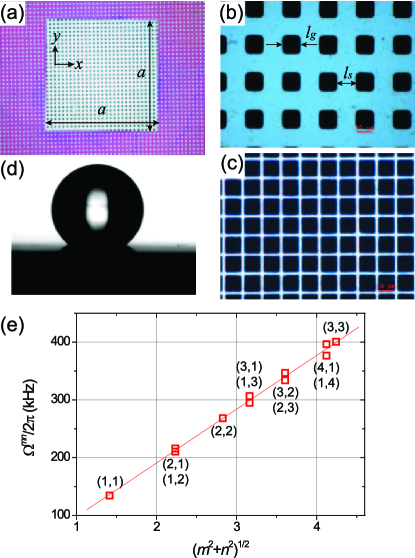
Figure 1: (a) Top view of a porous membrane chip ($a\times a=600\times 600$ $\mu{{\rm{m}}^{\rm{2}}}$). (b), (c) Optical micrographs of $\Phi_{s}=0.78$ and 0.34 membranes, respectively. (d) A drop of water placed on a larger membrane ($a\times a=2\times 2$ ${{\rm{mm}}^{\rm{2}}}$ and $\Phi_{s}=0.48$) showing the superhydrophobicity of the surface. (e) Vacuum mechanical resonances of a $600\times 600$ $\mu{{\rm{m}}^{\rm{2}}}$ porous membrane with $\Phi_{s}=0.34$. Nearly-degenerate modes $(m,n)$ and $(n,m)$ are observed when $m\neq n$. Single standard deviations in the data are smaller than the symbols.

On a conventional superhydrophobic surface degennesBOOK , hydrophobicity combined with microscopic roughness causes the water surface to remain suspended above the solid tips, with mostly trapped air underneath watanableLANGMUIR ; bicoEPL01 . Since the flow is on a composite surface made up of solid and air, one solves the Navier-Stokes equations subject to no-slip on the solid elements and to slip at the water-air interface laugaHANDBOOK . Thus, in a first pass analysis, viscous friction force on a superhydrophobic surface is found to be proportional to the wet solid area, $\Phi_{s}$ ybertPHYSFLUID04 . In this manuscript, we show that flow on a porous superhydrophobic membrane deviates from the above picture. Oscillatory hydrodynamic response ekinciLoC10 of the membrane suggests that a stable Knudsen layer of gas percolates on the membrane, changing the boundary condition. This is because the porous superhydrophobic membrane structure enables the surrounding air to move ballistically to the interface with little resistance — in contrast to a conventional superhydrophobic surface, where trapped gas pockets are diffusively connected to a gas reservoir through macroscopic distances.

The novel system under study shown in Fig. 1 is a tension-dominated porous silicon nitride membrane made hydrophobic by silanization. The membrane has a (nominal) macroscopic area of $a\times a=600\times 600$ $\mu{{\rm{m}}^{\rm{2}}}$ and a nanoscale thickness of $t_{s}=200$ nm. A matrix of identical square pores with dimensions $l_{g}\times l_{g}=10\times 10$ $\mu{{\rm{m}}^{\rm{2}}}$ are lithographically etched in the membrane. The pitch is $l_{g}+l_{s}$, where $l_{s}$ is the width of the solid strips in between the pores, as shown in Fig. 1(b). This results in a solid area fraction $\Phi_{s}=1-\frac{l_{g}^{2}}{(l_{g}+l_{s})^{2}}$. When a drop of water is placed on the porous membrane, it is supported by a composite surface of solid and gas (air); thus, wetting is not favored as shown in Fig. 1(d).

We first characterize the intrinsic mechanical properties of the porous membranes. In order to eliminate any fluidic effects, we perform these measurements under vacuum. For a tension dominated square membrane ($a\times a\times t_{s}$), the frequency of the normal mode $(m,n)$ in vacuum is given by ${{\Omega_{v}^{mn}}\over{2\pi}}={[{{{\sigma_{s}}{\pi^{2}}}\over{{\Phi_{s}}{\rho_{s}}{t_{s}}{a^{2}}}}({m^{2}}+{n^{2}})]^{1/2}}$ Timoshenko . Here, $\sigma_{s}$ is the tension, $\rho_{s}$ is the density, and $m$ and $n$ are two integers. The in vacuo mode frequencies $\Omega_{v}^{mn}\over 2\pi$ of a $\Phi_{s}=0.34$ membrane are shown in Fig. 1(e). Here, the resonances are excited by a piezoelectric-shaker and detected using a Michelson interferometer at a pressure of $10^{-2}$ Pa. The data confirm that the tension-dominated membrane approximation holds well, even for a membrane with a very small solid fraction. Given that the modes are well-separated in frequency, each mode $(m,n)$ can be modeled as a damped harmonic oscillator with effective mass $M_{s}=\frac{\rho_{s}\Phi_{s}t_{s}a^{2}}{4}$ and stiffness $K_{s}=\frac{\sigma_{s}\pi^{2}}{4}(m^{2}+n^{2})$. Relevant mechanical parameters for the fundamental modes of all our membranes are displayed in Table 1.

Table 1: Mechanical properties for the fundamental mode of the porous membranes.

$\Phi_{s}$	$\Omega^{11}/2\pi$	$K_{s}$	$M_{s}$
	(kHz)	(N/m)	($10^{-12}$ kg)
1	235	134	61.2
0.96	233	126	58.7
0.88	223	104.7	53.8
0.82	208	67.6	50.2
0.78	142	38.1	47.7
0.65	159	39.2	39.8
0.48	106	12.9	29.4
0.34	134	14.2	21.1

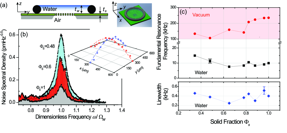
Figure 2: (a) Schematic of the measurement cell in cross-sectional and isometric views. The cell is filled with water and is placed on top of the membrane chip. A heterodyne Michelson interferometer probes the motion from below. (b) Thermal noise spectra of the fundamental mode of three different membranes with water atop. From top to bottom, $\Phi_{s}=$0.48, 0.6 and 1. The frequency axis is normalized with the respective resonance frequencies in water. The inset shows the shape of the fundamental mode for the $\Phi_{s}=0.6$ membrane. (c) Fundamental-mode resonance frequencies in vacuum and with water atop, and linewidths $\gamma_{w}/2\pi$ with water atop. Error bars represent the associated single standard deviations and are only shown when larger than the symbols.

We now turn to measurements with water. The measurements are performed using a fluid cell atop the membrane as shown in Fig. 2(a). The porous membrane does not leak but supports intimate and continuous contact with both the water reservoir above and the gas reservoir (ambient atmosphere) below. Using a heterodyne Michelson interferometer (with displacement sensitivity of 100 ${\rm{fm}}/\sqrt{{\rm{Hz}}}$ around 10 kHz with 85 $\mu$W incident on the photodetector), we have measured the thermal-noise spectra of all the membranes in their fundamental modes. Fig. 2(b) shows the noise spectra measured at the center of three membranes with different $\Phi_{s}$. In order to confirm that we are working with the fundamental mode [$(m,n)=(1,1)$], we have scanned the optical spot along the $x$ and $y$ directions and obtained mode shapes, such as the one shown in the inset of Fig. 2(b). Since we exclusively study the hydrodynamic response of the fundamental mode here, we henceforth drop the superscript 11. The top data trace in Fig. 2(c) shows all the fundamental resonance frequencies in vacuum, ${\Omega_{v}}\over{2\pi}$, obtained by driving the membranes linearly. Thermal spectra with water atop the membranes have provided the resonance frequencies ${\Omega_{w}}\over{2\pi}$ and linewidths $\gamma_{w}\over{2\pi}$ (bottom trace) Air .

We first provide a general discussion of the fluid dynamics encountered in our system. We consider the out-of-plane (broadside) oscillations of a rigid square ($a\times a$) plate immersed in a viscous fluid. We take the plate velocity as the real part of the complex exponential, ${{\bf{u}}_{\bf{s}}}=\Re\left\{{{U_{s}}{e^{i\omega t}}{\bf{\hat{z}}}}\right\}$, with amplitude $U_{s}$. Adopting the no-slip boundary condition, we find the magnitude of the fluidic force $F_{f}{\bf{\hat{z}}}$ on the plate in the high-frequency limit as ZhangStone

$${F_{f}}\approx\Re\left\{{A{{{\mu_{f}}{a^{2}}}\over\delta}{u_{s}}{e^{i\phi}}+M_{f}{{d{u_{s}}}\over{dt}}}\right\},$$ (1)

with $\phi\approx{{\pi}\over{4}}$ and $A\sim 20$. The viscous boundary layer thickness, $\delta=\sqrt{\frac{2\mu_{f}}{\rho_{f}\omega}}$, depends on the dynamic viscosity $\mu_{f}$ and density $\rho_{f}$ of the fluid. $M_{f}$ is the so-called added or hydrodynamic mass, well-known from the potential flow theory around an accelerating solid body. Consequences of Equation (1) are as follows. Viscous energy dissipation is due to tangential flow on the plate, expressed by the first term on the right-hand side. Being proportional to $\mu_{f}$, the dissipation provides a widely-used probe of the fluid-solid interaction. The second term on the right-hand side does not contribute to dissipation since $u_{s}{{d{u_{s}}}\over{dt}}$ integrated over a cycle is zero. However, this term provides an independent probe of the fluid properties (near the solid) through $\rho_{f}$. To emphasize this, we write $M_{f}=\rho_{f}V_{f}$, where $V_{f}$ stands for the volume of fluid displaced by plate motion and depends only upon geometry. Indeed, it will be shown below that, in our system, the changes in the nature of the fluid near the solid boundary results in changes in both $M_{f}$ and dissipation.

Returning to the membrane oscillations, we make a one-dimensional harmonic oscillator approximation for the fundamental mode. We analyze all our experimental data (of Fig. 2 and Table 1) using this approximation, obtaining the results shown in Fig. 3. In this approximation, the membrane has position $z_{s}$, velocity ${{\bf{u}}_{\bf{s}}}={\dot{z}_{s}}{\bf{\hat{z}}}$, mass $M_{s}$ and stiffness $K_{s}$. We assume that $u_{s}$ is nearly sinusoidal because all membrane resonances in water have quality factors $Q_{w}\gtrsim 20$ and the thermal drive has a white spectrum: $u_{s}\approx{\Re}\left\{{U_{s}{e^{i\Omega_{w}t}}}\right\}$. Given that the dissipation from water dominates the overall dissipation Air , we write ${M_{s}}\dot{u}_{s}\approx F_{e}+F_{w}$, where $F_{e}=-K_{s}z_{s}$ is the elastic spring force and $F_{w}=F_{f}$ in Eq. (1) with the appropriate parameters. Based on these considerations, we write a complex linear response function for the system as paul $G(\omega)\approx{[{K_{s}}-({M_{s}}+{M_{w}}){\omega^{2}}+i\alpha\omega]^{-1}}$. The effect of the fluid is embedded in two measurable parameters: the added water mass $M_{w}$ and the friction coefficient $\alpha$ reif .

The added water mass $M_{w}$ can be determined from the frequency shift of the membrane mode when it is loaded with water. The stiffness $K_{s}$ of the mode does not change appreciably from vacuum to water. Thus, ${M_{s}}{\Omega_{v}}^{2}=({M_{s}}+{M_{w}}){\Omega_{w}}^{2}$, which simplifies to ${M_{s}}{\Omega_{v}}^{2}\approx{M_{w}}{\Omega_{w}}^{2}$ since ${M_{s}}\ll M_{w}$ maali . Figure 3(a) shows $M_{w}$ as a function of $\Phi_{s}$, calculated using $M_{s}$ values in Table 1 and frequency values in Fig. 2(c). Note the two separate regions in Fig. 3(a) with a transition around $\Phi_{s}\approx 0.9$. In order to estimate $M_{w}$ from first principles, we emphasize that our resonator is not immersed in water [see Fig. 2(a)] — unlike in a typical set up. There is a water layer of thickness $t_{w}=2.4$ mm and density $\rho_{w}$ atop the membrane, but the backside is exposed to atmosphere. The dominant hydrodynamic mass contribution comes from the the entire water layer moving in-phase with the membrane in the $z$ direction shear-mass . This provides $M_{w}\approx{{\rho_{w}t_{w}a^{2}}\over{4}}\approx 2\times 10^{-7}$ kg [dotted segment in Fig. 3(a)]. This estimate is in agreement with the data of Fig. 3(a), but only in the region $0.9\leq\Phi_{s}\leq 1$. Further support for our estimate comes when $t_{w}$ is reduced to approximately 1.2 mm, which results in a factor of 1/2 reduction in $M_{w}$. Experimentally, the measured frequency increases by a factor of 1.2, which is close to the factor $\sqrt{2}$ expected. For $\Phi_{s}\lesssim 0.9$, there is a significant deviation from this simple model: the measured $M_{w}$ shows a rather fast decrease, eventually by a factor of 23.

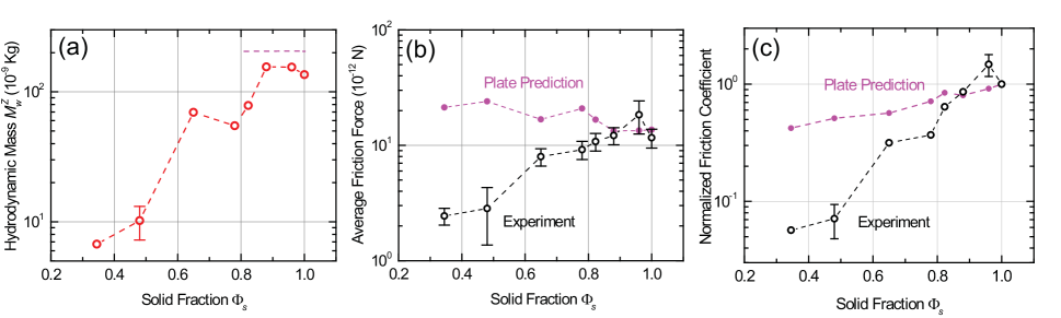
Figure 3: (a) Measured $M_{w}$ as a function of $\Phi_{s}$. The line segment is the hydrodynamic mass of the entire water layer. (b) Average friction force and (c) the normalized friction coefficient. The plate prediction is calculated from Eq. (1) using experimental velocities and frequencies where needed. The normalized friction coefficient for the plate model is $\approx\Phi_{s}$. Error bars represent the associated single standard deviations and are only shown when larger than the symbols.

The upper, slowly increasing trace in Fig. 3(b) is the cycle-averaged viscous force on the membrane, ${{A{\mu_{w}}{a^{2}}{\Phi_{s}}{U_{s}}}\over{2{\pi^{2}}\delta}}$, predicted using the plate model of Eq. (1) and accounting for the membrane mode-shape. Here, $\mu_{w}$ is the dynamic viscosity of water; ${A\over{2{\pi^{2}}}}\sim 1$; ${U_{s}}^{2}\approx 2{\pi^{2}}{\Omega_{w}}^{2}\left\langle{{{z_{s}}^{2}}}\right\rangle$, ${\left\langle{{z_{s}}^{2}}\right\rangle^{1/2}}$ being the thermal amplitude of the membrane found from the integral of the measured displacement noise spectral density. It is important to note that, as $\Phi_{s}$ becomes smaller, $U_{s}$ increases. This is because the stiffness $K_{s}$ decreases (see Table 1), the average thermal drive force remains constant and $\Omega_{w}$ changes very slowly. In the calculated plate model, the decrease in the wet area, $a^{2}\Phi_{s}$, appears to be off-set by this increase in $U_{s}$, thus resulting in a net increase in the drag force as $\Phi_{s}$ decreases. The experimental cycle-averaged friction force is obtained from the one-dimensional damped harmonic oscillator model as $\alpha U_{s}\approx M_{w}\gamma_{w}U_{s}$. This force plotted as the lower trace in Fig. 3(b) shows a surprising deviation from the plate model. As in added mass, the plate prediction agrees with the experiments when $\Phi_{s}\approx 1$. However, for $\Phi_{s}\lesssim 0.9$, the drag force decreases rapidly, attaining a value an order of magnitude smaller than the plate prediction at $\Phi_{s}=0.34$.

The drag reduction on the porous membranes can be better assessed, if one considers the drag force per unit velocity: this is the friction coefficient $\alpha$. Figure 3(c) shows the predicted and experimentally-obtained normalized friction coefficients, ${{\alpha({\Phi_{s}})}\over{\alpha(1)}}$. The predicted value is proportional to $\Phi_{s}$ since the system behaves as a plate, but with a reduced solid area. The experimental values are given by $\alpha\approx M_{w}\gamma_{w}$. The data show that drag force for a given velocity can be reduced by a factor of 18, if one goes from a complete membrane ($\Phi_{s}=1$) to $\Phi_{s}=0.34$, i.e., $\alpha(0.34)\approx\alpha(1)/18$.

Given that the the membranes do not leak and $M_{w}$ is constant for $0.9\leq{\Phi_{s}}\leq 1$, we conclude that the presence of the air reservoir does not affect the flow in this interval. The agrement between the predicted and measured friction forces in the same interval provides more support for this conclusion. The significant deviation in the measured response from the plate model for $\Phi_{s}\lesssim 0.9$ suggests that the flow changes around $\Phi_{s}\approx 0.9$. The new feature of our system is its openness to air at atmospheric pressure. The membrane thickness, $t_{s}=200$ nm, is close to the mean-free-path of air, $\lambda_{g}\approx 60$ nm. This enables the surrounding air to move through the membrane pores with little resistance. The dramatic decrease in $M_{w}$ for $\Phi_{s}<0.9$ can be attributed to a percolation transition: air bubbles localized within the well-defined pores begin to coalesce as $\Phi_{s}$ is decreased, eventually resulting in a complete gas layer, which separates the solid strips from the water surface. This gas layer is expected to exist in the Knudsen regime, with its thickness $\xi$ smaller than its mean-free-path, $\xi\lesssim\lambda_{g}$.

Assuming a complete Knudsen layer at the interface, we can assess the friction reduction on a porous membrane with small $\Phi_{s}$. A one-dimensional model will suffice. We consider a large porous plate oscillating in its plane with velocity, $\Re\left\{{{U_{s}}{e^{i\Omega_{w}t}}{\bf{\hat{x}}}}\right\}$, under water with a Knudsen air layer in between the plate and the water. The velocity field inside the water is ${\Re}\left\{{U_{w}{e^{-{z\over\delta}+i(\Omega_{w}t-{z\over\delta}))}}{\bf{\hat{x}}}}\right\}$ and $U_{w}\neq U_{s}$. Since the stress is a continuous function of coordinate at the interface ($z\approx 0$), ${{{\mu_{w}}{U_{w}}}\over\delta}\sim{{{\rho_{g}}{U_{s}}{\Phi_{s}}{u_{th}}}\over 6}$. Here, $U_{s}\Phi_{s}$ and $u_{th}$ are respectively the average hydrodynamic velocity and the thermal velocity of air molecules; $\rho_{g}$ is the density of air. The $1/6$ factor accounts for the fraction of molecules traveling in the $+z$ direction. Using the parameters available, we derive $\frac{U_{s}}{U_{w}}\sim\frac{3}{\Phi_{s}}$. The slip length laugaHANDBOOK , ${\lambda}\sim{{{\mu_{w}}}\over{{\rho_{g}}{u_{th}}{\Phi_{s}}}}$, emerges as 6 $\mu$m at $\Phi_{s}=0.34$.

Our results might be relevant to applications. Unlike air bubbles on a hydrophobic surface BrennerPRL08 , the air layer in our system is stable against diffusion into the water because of the resistance-free influx from the air reservoir. Assuming that porous pipes of macroscopic dimensions can be manufactured, significant drag reduction could be achieved. Several puzzling phenomena in bio-fluid-dynamics, including transport through and over bio-membranes, and propulsion over the water surface, may be related to the physics observed here Bush ; Gao .

The authors thank L. Chen and G. Holland for technical assistance, and J. A. Liddle and V. Aksyuk for fruitful discussions. Support from the US NSF (through grants ECCS-0643178, CBET-0755927, and CMMI-0970071) is acknowledged.

References

- (1) L.D. Landau, and E.M. Lifshitz, Fluid Mechanics (Butterworth-Heinemann, Oxford, 1987), 2nd ed.
- (2) E. Lauga, M. Brenner, and H.A. Stone, Handbook of Experimental Fluid Mechanics, edited by C. Tropea, A. L. Yarin, and J. F. Foss. Springer-Verlag, Berlin, 2007.
- (3) O.I. Vinogradova, Langmuir 11, 2213 (1995).
- (4) C.I. Bouzigues et al., Phil. Trans. R. Soc. A 366, 1455 (2008).
- (5) J.W.G. Tyrrell and P. Attard, Phys. Rev. Lett. 87, 176104 (2001).
- (6) X.H. Zhang, A. Khan, and W.A. Ducker, Phys. Rev. Lett. 98, 136101 (2007).
- (7) P. Joseph et al., Phys. Rev. Lett. 97, 156104 (2006).
- (8) C.H. Choi and C.J. Kim, Phys. Rev. Lett. 96, 066001 (2006).
- (9) C. Cottin-Bizonne et al., Nat. Mat. 2, 237 (2003).
- (10) A.M.J. Davis and E. Lauga, Phys. Fluids 21, 113101 (2009).
- (11) C. Neinhuis and W. Barthlott, Annals of Botany 79, 667 (1997).
- (12) J.W.M. Bush, D.L. Hu, and M. Prakash, Advances in Insect Physiology Volume 34, 117 (2007)
- (13) X. Gao, and L. Jiang, Nature 432, 36 (2004).
- (14) R.J. Daniello, N.E. Waterhouse, and J.P. Rothstein, Phys. Fluids 21, 085103 (2009).
- (15) P.G. de Gennes, F. Brochard-Wyart, and D. Quere, Capillarity and Wetting Phenomena: Drops, Bubbles, Pearls, Waves Springer, New-York, 2004.
- (16) M. Miwa et al., Langmuir 16, 5754 5760 (2000).
- (17) J. Bico, C. Tordeux, and D. Qur, Europhys. Lett. 55, 214 (2001).
- (18) C. Ybert et al., Phys. Fluids 19, 123601 (2007).
- (19) K.L. Ekinci et al., Lab Chip 10, 3013 (2010).
- (20) S. Timoshenko, D.H. Young, and W. Weaver, Jr., Vibration Problems in Engineering (John Wiley and Sons, 1974).
- (21) All in vacuo quality factors are in the range to . In air (without water), the resonance frequencies shift down from their vacuum values, while quality factors remain .
- (22) M.P. Brenner and D. Lohse, Phys. Rev. Lett. 101, 214505 (2008).
- (23) W. Zhang and H.A. Stone, J. of Fl. Mech. 367, 329 (1998).
- (24) M.R. Paul, M.T. Clark, and M.C. Cross, Nanotechnology 17, 4502 (2006).
- (25) The shear-induced added mass is negligibly small because m when .
- (26) F. Reif, Fundamentals of Statistical and Thermal Physics (New York, NY: McGraw-Hill, 1965).
- (27) A. Maali et al., J. Appl. Phys. 97, 074907 (2005)