Effect of Coulomb interactions on the physical observables of graphene

Abstract

We give an update of the situation concerning the effect of electron–electron interactions on the physics of the neutral graphene system at low energies. We revise old renormalization group results and the use of the 1/N expansion to address the questions of the possible opening of a low energy gap, and the magnitude of the graphene fine structure constant. We emphasize the role of the Fermi velocity as the only free parameter determining the transport and electronic properties of the graphene system and revise its renormalization by Coulomb interactions on the light of recent experimental evidences.

I Introduction

Graphene is considered to be a bridge between quantum field theory (QFT) and condensed matter physics due to the low energy description of the elementary excitations as massless Dirac fermions in two spacial dimensions. This description realizes some important toy models used to study quark confinement and chiral symmetry breaking in QFT, particularly Quantum Electrodynamics in two spacial dimensions QED(3) Schwinger (1962); Pisarski (1984). On the condensed matter point the QFT modeling of graphene raises two important questions: under a fundamental point of view it is not guaranteed that the neutral graphene system with Coulomb interaction is a Fermi liquid Landau (1957). On a more practical side, the QFT model has logarithmic divergences that need to be renormalized what introduces some subtleties in fixing the value of the graphene fine structure constant affecting the experiments.

Electron–electron interactions were considered to be very small or even absent in the first experiments Novoselov et al. (2004, 2005); Zhang et al. (2005); Jiang et al. (2007); Bostwick et al. (2007); Zhou et al. (2008); Li et al. (2009); Nair et al. (2008); Li et al. (2008) but the recent advances in the synthesis and the big improvement in the quality of the samples have changed this view. The observation of the fractional Quantum Hall effect Du et al. (2009); Bolotin et al. (2009) and the experiments probing the zero Landau level in high magnetic fields Gorbar et al. (2011) have renewed the interest on the role of Coulomb interactions on the intrinsic properties of the system. Since the role of many body corrections to the physics of graphene has been extensively studied in the literature (for a recent review see Kotov et al. (2010) and the references inside), we will here pick up these aspects that in our opinion are more interesting or less well understood. Here we just note that, since all other interactions are irrelevant at sufficiently low energies González et al. (1994); Vozmediano (2011), the Coulomb interaction is the only feature affecting the physical properties of the clean suspended samples.

The low energy effective model for graphene being a QFT model suffers from one typical problem: perturbation theory calculations of any observable quantity are plagued by infinities or spurious cutoff dependences. The standard QFT renormalization program allows us to address two very important questions in the physics of graphene: what is the strength of the Coulomb interaction at low energies - i. e. what is the actual value of the graphene fine structure constant –, and will the interactions lead to a band gap opening? We summarize the contents of this review by giving answers to these questions, the second first: A gap will not open in graphene at low energies for moderate values of the graphene fine structure constant $\alpha_{G}$. And: the infrared value of $\alpha_{G}$ is smaller than the assumed value based on a Fermi velocity of the order of $c/300$.

Note however that interactions are very much enhanced in the presence of strong magnetic fields. In this situation a gap can open at the neutrality point Checkelsky et al. (2008). This article describes the physical low energy properties of neutral, clean graphene at zero magnetic field.

II Graphene versus QED

II.1 The continuum model

One of the facts that has allowed the fast development in the understanding of the electronic properties of graphene is that there is a well established model Hamiltonian universally accepted by the community. This is another similarity with the physics of elementary particles. The standard non-interacting model for the electronic excitations around a single Fermi point in graphene (in units $\hbar=1$) is given by

$${\cal H}=v_{F}\int d^{2}{\bf r}\bar{\psi}({\bf r})\gamma^{i}\partial_{i}\psi({\bf r})\;,$$ (1)

where $i=1,2$, $\bar{\psi}({\bf r})=\psi^{+}({\bf r})\gamma^{0}$, and the gamma matrices can be chosen as $\gamma_{x}=\sigma_{2},\gamma_{y}=-\sigma_{1},\gamma^{0}=\sigma_{3}$ . $\sigma_{i}$ are the Pauli matrices and $v_{F}$ is the Fermi velocity, the only free parameter in the Hamiltonian. When promoting the Hamiltonian to a QFT action we have the electron wave function as an additional parameter defining the theory.

And the electron-electron interactions are described by the Hamiltonian

$${\cal H}_{\rm int}=e^{2}\int d^{2}{\bf r}d^{2}{\bf r^{\prime}}\frac{\psi^{+}({\bf r})\psi({\bf r})\psi^{+}({\bf r^{\prime}})\psi({\bf r^{\prime}})}{|{\bf r}-{\bf r^{\prime}}|}.$$ (2)

It is immediately seen that, unlike what happens in the usual two dimensional electron gas, the ratio of the Coulomb interactions and the kinetic energy in this system is a constant independent of the density and given by $g\sim\frac{e^{2}}{v_{F}}$ often taken as the graphene fine structure constant.

Since the model Hamiltonian is the relativistic Dirac Hamiltonian it saves a lot of efforts to adopt a covariant formulation and profit of the results already known in QFT. The fact that the numerical value of Fermi velocity does not equal the speed of light is not important, the model is still relativistic with a different light cone. What is very different and interesting under a QFT point of view is the fact that the velocity defining the light cone is renormalized by the interactions.

Following the quantum field theory nature of the model, we replace the instantaneous Coulomb interaction of eq. (2) by a local gauge interaction through a minimal coupling:

$$L_{\rm int}=g\int d^{2}xdtj^{\mu}(x,t)A_{\mu}(x,t)\;,$$

where the electron current is defined as

$$j^{\mu}=(\overline{\Psi}\gamma^{0}\Psi,v_{F}\overline{\Psi}\gamma^{i}\Psi)\;.$$

With this substitution we have formally an effective Lagrangean

$${\cal L}=\int d^{2}{\bf r}\;dt\;\bar{\psi}\;\gamma^{\mu}[\partial_{\mu}+ieA_{\mu}]\psi\;,$$ (3)

very similar to that of massless QED in two spatial dimensions. What makes the graphene model different from QED in any number of dimensions is the gauge boson propagator. As discussed at length in González et al. (1994); de Juan et al. (2010); Vozmediano (2011), a gauge field propagator in QFT has a $1/k^{2}$ dependence while the effective Coulomb interaction in graphene propagates as $1/k$. This is due to the fact that only the charges are confined to live in the two dimensional surface defined by the sample. The photons propagate in the three dimensional space. This is a crucial aspect that makes the model interesting and behaving more like the scale invariant massless QED(3+1) rather than the super–renormalizable QED(2+1). The renormalization of the Fermi velocity is a consequence of this fact.

II.2 Perturbative renormalization

In standard QED(4) there are three one loop diagrams that have logarithmic singularities (see Fig. 1) and three free parameters in the theory (the coupling constant and the electron and photon wave functions). The theory is strictly renormalizable in the sense that all divergences at any order in perturbation theory can be cured by a proper redefinition of the parameters. Subsequently the physical values of these parameters are fixed by experimental data (renormalization conditions). On the other hand, QED(3) is a super-renormalizable theory meaning that the coupling constant has dimensions of energy what improves the convergence of the perturbative series. It has less divergences and these can be properly renormalized. In fact, massless QED (2+1) is ultraviolet finite although it has infrared divergences Mitra et al. (2005). Graphene sits in between QED(3) and QED(4). Of the three graphs shown in Fig. 1 only the electron self–energy diverges and in the case of considering a static photon propagator only the spatial part has a logarithmic divergence.

Figure 1: Primitively divergent Feynman graphs in QED(4). Fermion self–energy (a), vertex (b) and photon self-energy (c).

In the static model, the electron and photon propagators in momentum space are given by

$$G_{0}(k^{0},{\bf k})=i\frac{\gamma^{0}k_{0}+v\bm{\gamma}\cdot{\bf k}}{-(k^{0})^{2}+v^{2}{\bf k}^{2}}\;,$$ (4)

$$\Pi_{0}({\bf k})=\dfrac{1}{2}\frac{1}{|{\bf k}|}\;.$$ (5)

The renormalization functions associated to the electron self-energy are defined as:

$$G_{0}^{-1}-\Sigma(k^{0},{\bf k})=Z_{\psi}^{-1/2}(k^{0},{\bf k})[k^{0}\gamma^{0}-Z_{v}(k^{0},{\bf k})v\bm{\gamma}\cdot{\bf k}],$$ (6)

The extra parameter $v$ appearing in (4) in the graphene case has an associated renormalization function $Z_{v}$ which is a new feature characteristic of graphene. In the Lorentz invariant massless QED in any dimensions, only the electron wave function renormalization is associated to the the electron self energy. The computation of the graph in Fig. 1 (a) gives

$$\Sigma^{(1)}(\mathbf{k})\sim\frac{g}{4}v\bm{\gamma}\cdot\mathbf{k}\log\frac{{\bf k}^{2}}{\Lambda^{2}},$$ (7)

where g is the coupling constant to be discussed later, and $\Lambda$ is a high energy cutoff. The logarithmic divergence can be fixed by redefining the fermion velocity $v$ which becomes, after finishing the renormalization procedure, energy-dependent. The result is by now well known:

$$\frac{v_{F}(E)}{v_{F}(E_{0})}=1-\frac{g}{16\pi}\log(E/E_{0}),$$ (8)

which relates the value of the Fermi velocity at an energy $E$, with that at a reference energy $E_{0}$, assuming that the two energies are sufficiently closed. Notice that $E_{0}$ is not a cutoff of the order of the bandwidth but any energy where the Fermi velocity is determined by experiments. The corresponding diagram in massless QED(3) does not have a logarithmic divergence because the photon propagator has an extra inverse power of momentum. In QED(4) this diagram induces a wave function renormalization. It is interesting to note that the electron charge in the graphene model is not renormalized (after fixing the velocity divergences, the photon self-energy is finite at all orders in perturbation theory) but the velocity renormalization induces a renormalization of the graphene structure constant. Since according to eq. (8) the Fermi velocity increases at decreasing energies, the effective coupling constant $g\equiv e^{2}/4\pi v_{F}$ decreases in the infrared making perturbation theory more accurate.

III The coupling constant of Coulomb interaction and perturbation theory

As mentioned in the introduction perturbation theory calculations of any observable quantity are plagued by infinities. Perturbative renormalization Collins (1984) is a well prescribed mechanism to get rid of the infinities and define a sensible predictive theory. In the graphene system we encounter an additional problem: The bare value of the graphene fine structure constant

$$\alpha_{G}=\frac{e^{2}}{4\pi v_{F}},$$ (9)

is not small. Plugging–in the value of the bare electron charge $e$ and the Fermi velocity measured in nanotube experiments Liang et al. (2001) $v_{F}\sim c/300$, $\alpha_{G}$ is estimated to be of the order of $\alpha_{G}\sim 2.3-2.5$.

III.1 Screening in graphene

The estimate of $\alpha$ described above precludes the use of perturbation theory. This problem is not so severe for samples on a substrate, where the substrate dielectric constant reduces the effective coupling constant:

$$\alpha_{G}=\frac{e^{2}}{4\pi\varepsilon_{G}v_{F}}.$$ (10)

where $\varepsilon_{G}$ includes intrinsic contributions and effects due to the environment in which graphene is immersed. A simple estimate gives $\varepsilon_{G}=(\varepsilon_{air}+\varepsilon_{subs})/2\sim 2-3$ for typical substrates. An interesting topic is the intrinsic screening due to the graphene layer itself. Internal excitations in three dimensional insulators lead to a finite dielectric constant, which reduces the effective charge of the mobile carriers. By extrapolating measurements of the excitation spectra in graphite, it has been proposed that similar effects lead to a large intrinsic dielectric constant in single layer grapheneReed et al. (2010), $\varepsilon_{G}\sim 13$.

It is interesting to note that internal excitations in insulators, including electron-hole pairs, can be described as polarizable dipoles, which induce a field ${\cal E}_{ind}(\vec{\bf q})\propto\left|\vec{\bf q}\right|^{2}{\cal E}_{ext}(\vec{\bf q})$, where $\vec{\bf q}$ is the momentum of the external field. In a two dimensional system dipoles induce a field which tends to zero at small momenta, so that they do not contribute to the dielectric constant. The only internal screening processes in graphene which can modify the dielectric constant are the excitations near the Dirac energy. Their one loop contribution to the polarizability is finite and it can be calculated analytically

$$\Pi({\bf k},\omega)=i\frac{e^{2}}{8}\frac{{\bf k}^{2}}{\sqrt{v_{F}^{2}{\bf k}^{2}-\omega^{2}}}\;.$$ (11)

This one loop result is independent on the nature of the interaction since only electron propagators appear in the calculation. The resulting dielectric constant is $\epsilon=1+(N\pi\alpha)/8$, where $N=4$ is the number of fermion flavors (see next section). The inclusion of low order ladder diagramsKotov et al. (2008) does not change significantly this value.

An independent estimate of $\alpha$ in graphene has been obtained from measurements of the carrier-plasmon interaction in samples with a finite carrier concentrationBostwick et al. (2010). The result, $\alpha\approx 2.2$ is consistent with the previous analysis.

IV Renormalization of the Fermi velocity. 1/N expansion

The first perturbative renormalization results on the running of the coupling constant in graphene were obtained in ref. González et al., 1994 on the basis that, even if initially the graphene coupling constant is not small, it runs towards small values in the infrared where perturbation theory can be trusted. The logarithmic renormalization described in Sect. II is a one loop RG result that assumes the coupling constant to be small.

A standard perturbative framework for strongly coupled fermionic theories is the $1/N$ expansion first proposed in relation with Quantum Cromodynamics (QCD) ’t Hooft (1974). $N$ is the number of fermionic species in the problem that in the case of graphene with the spin and valley degeneracies is $N=4$. This procedure was followed in the early publications González et al. (1996, 1999) and was later retaken in Foster and Aleiner (2008); Drut and Lahde (2009a); Gamayun et al. (2002).

The simplest non-perturbative calculation amounts to compute the graph in fig. 1 (a) substituting the photon propagator by the RPA result which is a resummation of the planar diagrams dominant in the 1/N approximation:

$${\cal P}(\omega,{\bf k})=\frac{-i}{2|{\bf k}|+\frac{e^{2}}{8}\frac{k^{2}}{\sqrt{v_{F}^{2}k^{2}-\omega_{k}^{2}}}}.$$ (12)

From that we get the following equation for the running Fermi velocity González et al. (1999); Foster and Aleiner (2008):

$$\frac{1}{v_{F}}\frac{\partial v_{F}}{\partial l}=-\frac{8}{\pi^{2}N}\big{(}1+\frac{\arccos g}{g\sqrt{1-g^{2}}}\big{)}+\frac{4}{\pi g},$$ (13)

where $g=\frac{Ne^{2}}{32v_{F}}$ (the large N limit amounts to take the limit $N\to\infty$ keeping $g$ fixed). As we see the dependence on $g$ is non-perturbative and the growth of the velocity at low energies is slightly different than that in (8).

Another interesting prediction done within this framework is the linear dependence of the quasiparticles lifetime with the energy González et al. (1996), a distinctive of the marginal Fermi liquid behavior Varma et al. (1989). Experimental evidences of this behavior have been described in Zhou et al. (2006); Jiang et al. (2007); Li et al. (2009); Knox et al. (2011).

V Renormalization of the Fermi velocity: experimental confirmation

The deduction of the values of the physical parameters from a given experimental measure is one of the most important aspects of the renormalization program. This is one of the issues where physics from different areas come into play, the best example being the determination of the fine structure constant of QED. By combining solid state measurements of the electron precession in magnetic fields or the quantum Hall effect, with theoretical QFT calculations of the anomalous magnetic moment of the electron we reach the actual precision of better than one part in a trillion Hanneke et al. (2008).

It is fair to say that the Fermi velocity plays in graphene a role similar to the effective mass in the standard Fermi liquid theory: it enters in the definition of almost all the phenomenological quantities and, as such, it permeates in the value of the experimental observations. Taking for granted a constant, absolute value for this parameter can misguide the interpretation of some experiments or hide interesting physical issues. There has been a very recent experimental report on the observation of the renormalization of the Fermi velocity Elias et al. (2011) confirming earlier more indirect evidences Bostwick et al. (2007); Li et al. (2008). This is a very important result which can also affect the interpretation of other experimental observations. On the conceptual point of view, the verification of the growth of the Fermi velocity at low energies is interesting not only for the condensed matter community but also for the high energy as a beautiful example of renormalization at work. Under a more applied point of view, the Fermi velocity being almost the only parameter of the graphene model, it affects most of the experimental findings. The recognition that it changes with the energy can offer new insights in the interpretation of infrared data.

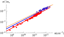
Figure 2: Experimental measurements of the effective mass of carriers in high mobility graphene samples. Red dots give results in suspended samples, and blue dots are for samples on BN substrates. The red and blue lines are fits using eq. 13. Red: $\varepsilon_{G}=1$. Blue: $\varepsilon_{G}=4$. The dotted orange line shows a fit obtained neglecting the renormalization of the Fermi velocity.

The renormalization predicted in eq. 13 is confirmed by the experimental results inElias et al. (2011). This reference reports measurements of the effective mass at different carrier densities for high mobility suspended graphene and graphene on BN. These experiments use the temperature dependence of Shubnikov-de Haas oscillations to infer the dependence of the Fermi energy, $\epsilon_{F}$, on the area of the Fermi surface, $S_{F}$. The effective mass is defined as

$$m_{eff} =\frac{\hbar^{2}}{2\pi}\frac{dS_{F}}{d\epsilon_{F}}$$ (14)

so that for graphene

$$m_{eff} =\frac{\hbar k_{F}}{v_{F}}$$ (15)

A comparison of experimental results an fits based in eq. 13 are shown in Fig. 2.

VI Opening a gap in graphene. Excitonic transition

Graphene is a semimetal and has zero gap. Under the QFT point of view, the electron mass (gap) is protected by the 3D version of chiral symmetry and hence a gap will not open by radiative corrections at any order in perturbation theory. Quantum electrodynamics (QED) in (2+1) dimensions has been studied at length in quantum field theory mostly in connection with dynamical mass generation Pisarski (1984); Appelquist and Pisarski (1981); Jackiw and Templeton (1981); Nash (1989) and confinement Polyakov (1975, 1977). Both problems are crucial in the physics of graphene, the first is related with the possibility of opening a gap in the system, the second one with the screening of the Coulomb interaction. A very interesting review on the QED properties of graphene and its possible dynamical mass generation can be found in Gusynin et al. (2007).

As mentioned in Sect. II, the coupling constant of QED(3) has dimensions of energy and, in this sense, mass generation is greatly facilitated since there is already a mass parameter in the theory. Even then, spontaneous chiral symmetry breaking in QED(3) in the 1/N approximation usually requires an unphysical number of fermionic species $N<2$ Appelquist et al. (1986).

The situation with graphene is even worse since there is no mass parameter to begin with. The simplest non-perturbative calculation that can be done to study the issue of the gap opening in graphene is the RPA type described in Sect. IV González et al. (1999). The absence of a constant term in the inverse electron propagator ensures that no mass is generated in this approximation. The 1/N expansion approach to the problem has been revised recently in González (2010) with the conclusion that a gap will not open for the physical values of the electronic degeneracy in graphene (N=4). A variational approach to the excitonic phase transition in graphene including the renormalization of the Fermi velocity Sabio et al. (2010) also produces quite negative results. A topological analysis of the stability of the Fermi points in graphene against gap opening was done in J. Mañes et al. (2007).

Despite these negative results, many reports on opening gaps in neutral graphene are found in the literature both on the experimental and theoretical sides. The possibility of an excitonic insulator was first suggested by Khveshchenko Khveshchenko (2001a, b) which also raised the issue of magnetic catalysis Gorbar et al. (2002) based on earlier studies of QED(2+1) Farakos et al. (1999).

The possibility of opening a gap when the substrate is commensurate with the lattice was suggested in J. Mañes et al. (2007) and given as a possible explanation of a gap observed in photoemission experiments on epitaxially grown grapheneZhou et al. (2007) and in scanning tunneling microscopy experiments of graphene on graphite Li et al. (2009). The influence of the substrate in this context has also been analyzed in Ratnikov (2008). Monte Carlo calculation in a lattice gauge theory framework predict the opening of a gap Drut and Lahde (2009b, a). A gap has been also claimed in very recent Angular resolved photoemission spectroscopy measurements of epitaxial graphene upon dosing with small amounts of atomic hydrogen Bostwick et al. (2009). Disorder can give rise to various strong coupling phases Stauber et al. (2005); Foster and Aleiner (2008); Herbut et al. (2009) whose physical properties only been partially explored Herbut et al. (2008).

The issue of the gap opening in single layer graphene remains open and some experimental effort is needed to dillucidate it. The situation in the bilayer McCann and Fal’ko (2006); Castro et al. (2007) is more clear because the gap is not protected there, short range interactions can be active at low energies and gaps can open in various ways Castro et al. (2007); Oostinga et al. (2008); Abergel and Chakraborty (2009); Barlas and Yang (2009); Feldman et al. (2009); Gorbar et al. (2010); Xu et al. (2010); Wang and Chakraborty (2010); Weitz et al. (2010); Nandkishore and Levitov (2010).

VII Retarded Coulomb interaction. Emergent Lorentz covariance

As we have discussed, in the static model commonly used in graphene with an instantaneous photon propagator, the Fermi velocity grows without bound in the infrared González et al. (1994). This sets a lower bound on the validity of the model that breaks down when the Fermi velocity approaches the speed of light $c$. The scale defines an infrared cutoff $\delta$ for the theory, and can be computed as:

$$\delta=k_{R}\exp\left[-\frac{16\pi(c-v(k_{R}))}{e^{2}}\right],$$ (16)

where $k_{R}$, $v_{R}$ are the renormalization condition chosen to define the theory. A typical estimate will of course produce an energy of approximately 100 orders of magnitude below $k_{R}$. This discussion is very similar to that leading to the Landau pole of QED Bogoliubov and Shirkov (1980) and simply points to the incompleteness of the theory. In our case there are physical low energy bounds much less stringent than that, preventing to access the infrared region. But even if this does not impose any real bound on the validity of the model from a experimental point of view, it is interesting to know that a complete theory exists of which the static limit is only an approximation.

In the retarded model González et al. (1994); Giuliani et al. (2010) the Fermi velocity does not run without stop. The beta function of the Fermi velocity has a non–trivial fixed point and the value of $v_{F}$ at the fixed point is precisely the speed of light $c$. This is a very neat example of emergent Lorentz symmetry.

VIII Discussion

The most important parameter in the computation of the observable quantities in graphene is the renormalized Fermi velocity that defines, together with the polarizability, the Coulomb coupling constant.

The program to fix this constant must be similar to the one followed in the case of the electromagnetic fine structure constant Hanneke et al. (2008). In the case of graphene the theoretical determination is much simpler since there are no mass parameters relations involved in the calculations. Moreover we have the additional fact that the quantity determining $\alpha_{G}$ (Fermi velocity) is by itself an observable related to the one particle properties of the system. We expect that a proper combination of photoemission Zhou et al. (2006); Bostwick et al. (2007) optical Nair et al. (2008) and transport Li et al. (2009); Du et al. (2008); Elias et al. (2011) measures with the corresponding calculations in the QFT renormalization scheme should be enough to determine $\alpha_{G}$ as precisely as needed both theoretically and experimentally, similarly to what happens in QED(3+1).

IX Acknowledgments

Support by MEC (Spain) through grants FIS2008-00124, PIB2010BZ-00512 is acknowledged.

References

- Schwinger (1962) J. Schwinger, Phys. Rev. 128, 2425 (1962).
- Pisarski (1984) R. Pisarski, Phys. Rev. D 29, 2423 (1984).
- Landau (1957) L. D. Landau, Soviet Physics JETP 3, 920 (1957).
- Novoselov et al. (2004) K. S. Novoselov, A. K. Geim, S. V. Morozov, D. Jiang, Y. Zhang, S. V. Dubonos, I. V. Gregorieva, and A. A. Firsov, Science 306, 666 (2004).
- Novoselov et al. (2005) K. S. Novoselov, A. K. Geim, S. V. Morozov, D. Jiang, M. I. Katsnelson, I. V. Grigorieva, S. V. Dubonos, and A. A. Firsov, Nature 438, 197 (2005).
- Zhang et al. (2005) Y. Zhang, Y.-W. Tan, H. L. Stormer, and P. Kim, Nature 438, 201 (2005).
- Jiang et al. (2007) Z. Jiang, E. A. Henriksen, L. C. Tung, Y.-J. Wang, M. E. Schwartz, M. Han, P. Kim, and H. L. Stormer, Phys. Rev. Lett. 98, 197403 (2007).
- Bostwick et al. (2007) A. Bostwick, T. Ohta, T. Seyller, K. Horn, and E. Rotenberg, Nature Physics 3, 36 (2007).
- Zhou et al. (2008) S. Zhou, D. Siegel, A. Fedorov, and A. Lanzara, Phys. Rev. B 78, 193404 (2008).
- Li et al. (2009) G. Li, A. Luican, and E. Andrei, Phys. Rev. Lett. 102, 176804 (2009).
- Nair et al. (2008) R. Nair, P. Blake, A. Grigorenko, K. Novoselov, T. Booth, T. Stauber, N. Peres, and A. Geim, Science 320, 1308 (2008).
- Li et al. (2008) Z. Q. Li, E. A. Henriksenand, Z. Jiang, Z. Ha, M. C. Martin, P. Kim, H. L. Stormer, and D. N. Basov, Nature Phys. 4, 532 (2008).
- Du et al. (2009) X. Du, I. Skachko, F. Duerr, A. Luican, and E. Andrei, Nature 462, 192 (2009).
- Bolotin et al. (2009) K. I. Bolotin, F. Ghahari, M. D. Shulman, H. L. Stormer, and P. Kim, Nature 462, 196 (2009).
- Gorbar et al. (2011) E. Gorbar, V. Gusynin, V. Miransky, and I. Shovkovy, arXiv:1105.1360 (2011).
- Kotov et al. (2010) V. Kotov, B. Uchoa, V. M. Pereira, A. H. C. Neto, and F. Guinea, arXiv:1012.3484 (2010).
- González et al. (1994) J. González, F. Guinea, and M. A. H. Vozmediano, Nucl. Phys. B 424 [FS], 595 (1994).
- Vozmediano (2011) M. A. H. Vozmediano, Phil. Trans. R. Soc. A 369, 2625 (2011).
- Checkelsky et al. (2008) J. G. Checkelsky, L. Li, and N. P. Ong, Phys. Rev. Lett. 100, 206801 (2008).
- de Juan et al. (2010) F. de Juan, A. G. Grushin, and M. Vozmediano, Phys. Rev. B 82, 125409 (2010).
- Mitra et al. (2005) I. Mitra, R. Ratabolea, and H. Sharatchandraa, Phys. Lett. B 611, 289 (2005).
- Collins (1984) J. Collins, Renormalization (Cambridge University Press, 1984).
- Liang et al. (2001) W. Liang, M. Bockrath, D. Bozovic, J. H. Hafner, M. Tinkham, and H. Park, Nature 411, 665 (2001).
- Reed et al. (2010) J. P. Reed, B. Uchoa, Y. I. Joe, Y. Gan, D. Casa, E. Fradkin, and P. Abbamonte, Science 330, 805 (2010).
- Kotov et al. (2008) V. N. Kotov, B. Uchoa, and A. H. C. Neto, Phys. Rev. B 78, 035119 (2008).
- Bostwick et al. (2010) A. Bostwick, F. Speck, T. Seyller, K. Horn, M. Polini, R. Asgari, A. H. MacDonald, and E. Rotenberg, Science 328, 999 (2010).
- ’t Hooft (1974) G. ’t Hooft, Nucl. Phys. B 72, 461 (1974).
- González et al. (1996) J. González, F. Guinea, and M. A. H. Vozmediano, Phys. Rev. Lett. 77, 3589 (1996).
- González et al. (1999) J. González, F. Guinea, and M. A. H. Vozmediano, Phys. Rev. B 59, R2474 (1999).
- Foster and Aleiner (2008) M. S. Foster and I. L. Aleiner, Phys. Rev. B 77, 195413 (2008).
- Drut and Lahde (2009a) J. Drut and T. A. Lahde, Phys.Rev. B 79, 165425 (2009a).
- Gamayun et al. (2002) O. V. Gamayun, E. V. Gorbar, and V. P. Gusynin, Phys. Rev. B 81, 075429 (2002).
- Varma et al. (1989) C. M. Varma, P. B. Littlewood, S. Schmitt-Rink, E. Abrahams, and A. E. Ruckenstein, Phys. Rev. Lett. 63, 1996 (1989).
- Zhou et al. (2006) S. Zhou, G.-H. Gweon, J. Graf, A. Fedorov, C. Spataru, R. Diehl, Y. Kopelevich, D.-H. Lee, S. G. Louie, and A. Lanzara, Nature Phys. 2, 595 (2006).
- Knox et al. (2011) K. R. Knox, A. Locatelli, M. B. Yilmaz, D. Cvetko, T. O. Mentes, M. A. N. no, P. Kim, A. Morgante, and R. M. Osgood, arXiv:1104.2551 (2011).
- Hanneke et al. (2008) D. Hanneke, S. Fogwell, and G. Gabrielse, Phys. Rev. Lett. 100, 120801 (2008).
- Elias et al. (2011) D. C. Elias, R. V. Gorbachev, A. S. Mayorov, S. V. Morozov, A. A. Zhukov, P. Blake, K. S. Novoselov, A. K. Geim, and F. Guinea, arXiv:1104.1396 (2011).
- Appelquist and Pisarski (1981) T. Appelquist and R. Pisarski, Physical Review D 23, 2305 (1981).
- Jackiw and Templeton (1981) R. Jackiw and S. Templeton, Physical Review D 23, 2291 (1981).
- Nash (1989) D. Nash, Phys. Rev. Lett. 62, 3024 (1989).
- Polyakov (1975) A. Polyakov, Phys. Lett. B 59, 82 (1975).
- Polyakov (1977) A. Polyakov, Nucl. Phys. B 120, 429 (1977).
- Gusynin et al. (2007) V. P. Gusynin, S. G. Sharapov, and J. P. Carbotte, Int. J. Mod. Phys. B 21, 4611 (2007).
- Appelquist et al. (1986) T. Appelquist, M. J. Bowick, D. Karabali, and L. C. R. Wijewardhana, Phys. Rev. D 33, 3774 (1986).
- González (2010) J. González, Phys.Rev. B 82, 155404 (2010).
- Sabio et al. (2010) J. Sabio, F. Sols, and F. Guinea, Phys. Rev. B 82, 121413(R) (2010).
- J. Mañes et al. (2007) J. Mañes, F. Guinea, and M. A. H. Vozmediano, Phys. Rev. B 75, 155424 (2007).
- Khveshchenko (2001a) D. V. Khveshchenko, Phys. Rev. Lett. 87, 246802 (2001a).
- Khveshchenko (2001b) D. V. Khveshchenko, Phys. Rev. Lett. 87, 206401 (2001b).
- Gorbar et al. (2002) E. V. Gorbar, V. P. Gusynin, V. A. Miransky, and I. A. Shovkovy, Phys. Rev. B 66, 045108 (2002).
- Farakos et al. (1999) K. Farakos, G. Koutsoumbas, and N. E. Mavromatos1, Phys. Lett. B 431, 147 (1999).
- Zhou et al. (2007) S. Y. Zhou, G. H. Gweon, A. V. Fedorov, P. N. First, W. A. De Heer, D. H. Lee, F. Guinea, A. H. Castro Neto, and A. Lanzara, Nature Mat. 6, 770 (2007).
- Ratnikov (2008) P. V. Ratnikov, JETP Lett. 87, 292 (2008), eprint arXiv:0805.451.
- Drut and Lahde (2009b) J. Drut and T. A. Lahde, Phys.Rev. Lett. 102, 026802 (2009b).
- Bostwick et al. (2009) A. Bostwick, J. L. McChesney, K. V. Emtsev, T. Seyller, K. Horn, S. D. Kevan, and E. Rotenberg, Phys. Rev. Lett. 103, 056404 (2009).
- Stauber et al. (2005) T. Stauber, F. Guinea, and M. A. H. Vozmediano, Phys. Rev. B 71, 041406(R) (2005).
- Herbut et al. (2009) I. F. Herbut, V. Juricic, and O. Vafek, Phys. Rev. B 80, 075432 (2009).
- Herbut et al. (2008) I. F. Herbut, V. Juricic, and O. Vafek, Phys. Rev. Lett. 100, 046403 (2008).
- McCann and Fal’ko (2006) E. McCann and V. I. Fal’ko, Phys. Rev. Lett. 96, 086805 (2006).
- Castro et al. (2007) E. V. Castro, K. S. Novoselov, S. V. Morozov, N. M. R. Peres, J. Lopes dos Santos, J. Nilsson, F. Guinea, A. K. Geim, and A. H. C. Neto, Phys. Rev. Lett. 99, 216802 (2007).
- Oostinga et al. (2008) J. B. Oostinga, H. B. Heersche, X. Liu, A. F. Morpurgo, and L. M. K. Vandersypen, Nat. Mater 7 7, 151 (2008).
- Abergel and Chakraborty (2009) D. S. L. Abergel and T. Chakraborty, Phys. Rev. Lett. 102, 056807 (2009).
- Barlas and Yang (2009) Y. Barlas and K. Yang, Phys. Rev. B 80, 161408(R) (2009).
- Feldman et al. (2009) B. E. Feldman, J. Martin, and A. Yacoby, Nature Phys. 5, 889 (2009).
- Gorbar et al. (2010) E. V. Gorbar, V. P. Gusynin, and V. A. Miransky, Pis’ma v ZhETF 91, 334 (2010).
- Xu et al. (2010) H. Xu, T. Heinzel, A. A. Shylau, and I. V. Zozoulenko, Phys. Rev. B 82, 115311 (2010).
- Wang and Chakraborty (2010) X. F. Wang and T. Chakraborty, Phys. Rev. B 81, 081402 (2010).
- Weitz et al. (2010) R. T. Weitz, M. T. Allen, B. E. Feldman, J. Martin, and A. Yacoby (2010), eprint arXiv:1010.0989.
- Nandkishore and Levitov (2010) R. Nandkishore and L. Levitov, Phys. Rev. B 82, 115431 (2010).
- Bogoliubov and Shirkov (1980) N. Bogoliubov and D. Shirkov, Introduction to the theory of quantized fields, 3rd edition (Wiley/Interscience, New York, 1980).
- Giuliani et al. (2010) A. Giuliani, V. Mastropietro, and M. Porta, Phys. Rev. B 82, 121418(R) (2010).
- Du et al. (2008) X. Du, I. Skachko, A. Barker, and E. Y. Andrei, Nature Nanotechnology 3, 491 (2008).