Fermions Analysis of IR modified Ho$\check{r}$ava-Lifshitz gravity: Tunneling and Perturbation Perspectives

Abstract

In this paper, we investigate the fermions Hawking radiation and quasinormal modes in infra-red modified Ho$\check{r}$ava-Lifshitz gravity under tunneling and perturbation perspectives. Firstly, through the fermions tunneling in IR modified Ho$\check{r}$ava-Lifshitz gravity, we obtain the Hawking radiation emission rate, tunneling temperature and entropy for the Kehagias-Sfetsos black hole. It is found that the results of fermions tunneling are in consistence with the thermodynamics results obtained by calculating surface gravity. Secondly, we numerically calculate the lowing quasinormal modes frequencies of fermions perturbations by using WKB formulas including the third orders and the sixth orders approximations simultaneously. It turns out that the actual frequency of fermions perturbation is larger than in the Schwarzschild case, and the damping rate is smaller than for the pure Schwarzschild. The resluts of fermions perturbation suggest the quasinormal modes could be lived more longer in Ho$\check{r}$ava-Lifshitz gravity.

I Introduction

Recently, Ho$\check{r}$ava presented a power counting renormalizable gravity theory at Lifshitz point which is called Ho$\check{r}$ava-Lifshitz (HL) gravity Horava11 . It exhibits a broken Lorentz symmetry at short distances and reduces to usual general relativity (GR) gravity at the large distances with particular $\lambda=1$ which controls the contribution of the extrinsic curvature trace. With HL gravity theory putting forth, HL gravity is intensively investigated in many aspects involving basic formalism basicformalism , cosmology cosmology , various black hole solutions and their thermodynamics BHsolutions ; Kehagias ; added1 ; added2 and so on.

In the subsequent developments of the HL gravity, people are trying to find the influence of matter fields for HL gravity. Which analogue of the matter energy-momentum tensor could be used to act gravitational source as GR? The pioneering works involve the geodesic analysis by various methods including the optical limit of a scalar field theory Capasso , super Hamiltonian formalism Rama , foliation preserving diffeomorphisms Mosaffa , Lorentz-violating Modified Dispersion Relations Sindoni an so on. The optical limit presented by Capasso and Polychronakos Capasso could offer a deformed geodesic equation by the generalized Klein-Gordon action. It is shown that the particles maybe does not move along geodesic. Deviations from geodesic motion appear both in flat and Schwarzschild-like spacetimes. Similar result deviations from GR also is found in Rama ; Mosaffa ; Sindoni with various above-mentioned approaches.

Considering vanishing cosmological constant ($\Lambda_{W}$), Kehagias and Sfetsos Kehagias proposes an asymptotically flat black hole solution by introducing the addition term proportional to the Ricci scalar of three geometry $\mu^{4}R^{(3)}$, which indicates the Minkowski vacuum and modified GR at infra-red (IR) modification. Then after that, many people have devoted to its phenomenology involving strong field gravitational lensingKonoplya2 ; sbchen , scalar field quasi-normal modesKonoplya2 ; sbchenqnm , timelike geodesic motion jhchen , thin accretion diskHarko1 and observations constraints xianzhiguance as well as its thermodynamics analysis Myung1 ; GUPjieshi1 ; castingjieshi2 , which presents the black hole entropy $S=A/4+\pi/\alpha\ln(A/4)$ via the first law of thermodynamics where $\alpha$ is Ho$\check{r}$ava parameter. This entropy could be treated as Generalized uncertainty principle quantum correction entropy GUPjieshi1 or casting entropy castingjieshi2 . If fermions are tunneling in this kind HL gravity, might it keep this logarithm entropy? Motivated by this, we investigate fermions tunneling in section III.

On the other hand, as we know that through some additional fields (e.g. scalar or fermions fields), the black hole suffers a damping oscillation phase which is named as “quasi-normal models” (QNMs) or “quasi-normal ringing”. As a results, the normal model oscillation is replaced by a complex frequencies which encodes the black hole’s important information such as mass, charge, momentum and the dimensions of spacetime. The real part of complex frequency represents the actual frequency and the imaginary part of its represents the damping of the oscillation. It is believed that these QN frequencies could be detected by (LIGO, VIRGO, TAMT, GEO600) in future. So according to this observable QNMs, some people have used massless scalar field to obtain the important lowing QN frequencies which could live longer and be detected easily Konoplya2 ; sbchenqnm . It is interesting that the QNMs of massless scalar field are longer lived and have larger real oscillation frequency in Ho$\check{r}$ava-Lifshitz gravity than in GR. Else, as one kind of basic particles, the fermions could offer us many important information. Motivated by the situations above, we will evaluate the QNMs for the massless fermions perturbations in section IV.

As we have already known that, due to the different kinetic terms, Ho$\check{r}$ava-Lifshitz gravity with $\lambda\neq 1$ is different significantly from General Relativity. Hence, the HL gravity with $\lambda\neq 1$ has been extensively studied in the literatures. The relevant works are mainly concentrated on the basic problems such as how to find various exact black hole solutions, the application of cosmology, the constraints of various fundamental parameters and so on. Despite more attention has been paid to the properties of HL black holes, there are a few works referring to the fermions analysis, especially to the $\lambda\neq 1$ case. So far as we know, the works relevant the fermion analysis focus mainly on the IR modified HL gravity including Dirac perturbations added31 ; added32 and fermion tunnelling for $z=4$ black holes added33 and so on. In Wang and Gui’s work added31 , the quasinormal frequencies of massless Dirac field perturbation are evaluated by third-order WKB approximation. In Varghese and Kuriakose’s work added32 , the evolution of Dirac perturbations is also investigated by using time domain integration and third-order WKB methods. In Chen, Yang and Zu’s work added33 , the fermion tunnelling is investigated in the background of (3 + 1) dimensions and (4 + 1) dimensions black holes in the $z=4$ HL gravity.

This paper is organized as follows. In section II, we present the Kehagias and Sfetsos black hole solutions. In section III, we calculate the fermions tunneling emission rate of Hawking radiation, tunneling temperature and entropy. In section IV, we use the third and the sixth orders WKB formulas to numerically calculate frequencies simultaneously. Section V is the conclusions. We adopt the signature $(-,+,+,+)$ and put $\hbar$, $c$, and $G$ equal to unity.

II An asymptotically flat infra-red modified black hole solution in deformed Ho$\check{r}$ava-Lifshitz gravity

In this section, we review briefly the KS black hole solutions under the limit of $\Lambda_{W}\longrightarrow 0$ with running constant $\lambda=1$ in the IR critical point $z=1$. The space geometric is parameterized with Arnowitt-Deser-Misner (ADM) formalism,

$$ds^{2}=-N^{2}dt^{2}+g_{ij}\left(dx^{i}+N^{i}dt\right)\left(dx^{j}+N^{j}dt\right).$$ (1)

The action for the fields of HL theory is

$$S = \int dtd^{3}x\sqrt{g}N\bigg{\{}\frac{2}{\kappa^{2}}\left(K_{ij}K^{ij}-\lambda K^{2}\right)-\frac{\kappa^{2}}{2\alpha^{4}}C_{ij}C^{ij}+\frac{\kappa^{2}\mu}{2\alpha^{2}}\epsilon^{ijk}R_{il}^{(3)}\nabla_{j}R^{(3)l}_{\ \ \ \ k}$$ (2)

$$\ \ \ \ \ \ \ \ \ \ \ \ \ \ \ \ \ \ \ -\frac{\kappa^{2}\mu^{2}}{8}R_{ij}^{(3)}R^{(3)ij}+\frac{\kappa^{2}\mu^{2}}{8\left(1-3\lambda\right)}\left(\frac{1-4\lambda}{4}\left(R^{(3)}\right)^{2}+\Lambda_{W}R^{(3)}-3\Lambda^{2}_{W}\right)+\mu^{4}R^{(3)}\bigg{\}},$$

where the second fundamental form, extrinsic curvature $K_{ij}$, and the Cotton tensor $C^{ij}$ are given as follows,

$$K_{ij} = \frac{1}{2N}\left(\frac{\partial}{\partial t}g_{ij}-\nabla_{i}N_{j}-\nabla_{j}N_{i}\right),$$ (3)

$$C^{ij} = \epsilon^{ikl}\nabla_{k}\left(R^{(3)j}_{l}-\frac{1}{4}R^{(3)}\delta_{l}^{j}\right).$$ (4)

Here, $\kappa$, $\lambda$, $\alpha$, $\mu$ and $\Lambda_{W}$ are the constant parameters. The last term of metric Eq.(2) represents a soft violation of the detailed balance condition. Comparing the HL gravity action with that of GR gravity, we can obtain the speed of light $c$, the Newton’s constant $G$ and the cosmological constant $\Lambda$

$$c=\frac{\kappa^{2}\mu}{4}\sqrt{\frac{\Lambda_{W}}{1-3\lambda}},\ \ G=\frac{\kappa^{2}}{32\pi c},\ \ \Lambda=\frac{3}{2}\Lambda_{W}.$$ (5)

In the limit of $\Lambda_{W}\longrightarrow 0$, we can obtain a deformed action as follows,

$$S = \int dt_{L}d^{3}x\left(\mathcal{L}_{0}+\mathcal{L}_{1}\right),$$ (6)

$$\mathcal{L}_{0} = \sqrt{g}N\bigg{\{}\frac{2}{\kappa^{2}}\left(K_{ij}K^{ij}-\lambda K^{2}\right)\bigg{\}},$$ (7)

$$\mathcal{L}_{1} = \sqrt{g}N\bigg{\{}\frac{\kappa^{2}\mu^{2}\left(1-4\lambda\right)}{32\left(1-3\lambda\right)}\mathcal{R}^{2}-\frac{\kappa^{2}}{2\alpha^{4}}\left(C_{ij}-\frac{\mu\alpha^{2}}{2}R_{ij}\right)\left(C^{ij}-\frac{\mu\alpha^{2}}{2}R^{ij}\right)+\mu^{4}\mathcal{R}\bigg{\}}.$$ (8)

For the particular case of $\lambda=1$ with $\alpha=16\mu^{2}/\kappa^{2}$, a spherically symmetric black hole solution is presented by Kehagias and Sfetsos Kehagias , which also is corresponding to an asymptotically flat space,

$$ds^{2}=-f(r)dt^{2}+\frac{dr^{2}}{f(r)}+r^{2}\left(d\theta^{2}+\sin^{2}\theta d\varphi^{2}\right).$$ (9)

The lapse function is

$$f(r)=1+\alpha r^{2}-\sqrt{r\left(\alpha^{2}r^{3}+4\alpha M\right)},$$ (10)

where the parameter $M$ is an integration constant related with the mass of black hole. Using the null hypersurface condition, one can find there are two horizons, inner $r_{-}$ and outer event horizon $r_{+}$ in this space,

$$r_{\pm}=M\left(1\pm\sqrt{1-\frac{1}{2\alpha M^{2}}}\right).$$ (11)

Thermodynamic quantities including mass $M_{KS}$, temperature $T_{KS}$, and heat capacity $C_{KS}$ and entropy $S_{KS}$ presented in Refs.Myung1 are listed as,

$$M_{KS} = \frac{1+2\alpha r_{\pm^{2}}}{4\alpha r_{\pm}},$$ (12)

$$T_{KS} = \frac{2\alpha r_{+}^{2}-1}{8\pi r_{+}(\alpha r_{+}^{2}+1)},$$ (13)

$$C_{KS} = -\frac{2\pi}{\alpha}\left[\frac{(\alpha r_{+}^{2}+1)^{2}(2\alpha r_{+}^{2}-1)}{2\alpha^{2}r_{+}^{4}-5\alpha r_{+}^{2}-1}\right],$$ (14)

$$S_{KS} = \frac{A}{4}+\frac{\pi}{\alpha}\ln\left(\frac{A}{4}\right),$$ (15)

with horizon area $A=4\pi r_{+}^{2}$. Under the limit of $\alpha\longrightarrow+\infty$, the entropy reduces to Bekenstein-Hawking entropy $S_{BH}=A/4$ for Schwarzschild black hole.

III fermions tunneling of IR modified Ho$\check{r}$ava-Lifshitz gravity

In this section, we investigate the Hawking radiation of Kehagias and Sfetsos black hole in IR modified Ho$\check{r}$ava-Lifshitz gravity with fermion tunneling. The tunneling probability, temperature and entropy are expected to be obtained. The Dirac equation in the KS black hole spacetime can be written as

$$\left[\gamma^{a}e_{a}^{\mu}\left(\partial_{\mu}+\Gamma_{\mu}\right)+\frac{m}{\hbar}\right]\Psi=0,$$ (16)

where $m$ is the mass of fermions. $e_{a}^{\mu}$ is the inverse of the tetrad $e^{a}_{\mu}$ defined by black hole metric $g_{\mu\nu}=\eta_{ab}e^{a}_{\mu}e^{b}_{\nu}$ with Minkowski metric $\eta_{ab}=\text{diag}(-1,1,1,1)$. $\gamma^{a}$ is the Dirac matrix and $\Gamma_{\mu}$ is the spin connection given by

$$\Gamma_{\mu}=\frac{1}{8}\left[\gamma^{a},\gamma^{b}\right]e_{a}^{\nu}e_{b\nu;\mu},$$ (17)

where the covariant derivative of $e_{b\nu}$ is given by Christoffel symbols $\Gamma_{\mu\nu}^{a}$ as,

$$e_{b\nu;\mu}=\partial_{\mu}e_{b\nu}-\Gamma_{\mu\nu}^{a}e_{ba}.$$ (18)

We choose following $\gamma$ matrix,

$$\gamma^{0}=\begin{pmatrix}-i&0\\ 0&i\end{pmatrix},\gamma^{1}=\begin{pmatrix}0&-i\sigma^{3}\\ i\sigma^{3}&0\end{pmatrix},\gamma^{2}=\begin{pmatrix}0&-i\sigma^{2}\\ i\sigma^{2}&0\end{pmatrix},\gamma^{3}=\begin{pmatrix}0&-i\sigma^{1}\\ i\sigma^{1}&0\end{pmatrix},$$ (19)

where $\sigma^{i}$ is Pauli sigma matrix,

$$\sigma^{1}=\begin{pmatrix}0&\ \ 1\\ 1&\ \ 0\end{pmatrix},\sigma^{2}=\begin{pmatrix}0&-i\\ i&\ \ 0\end{pmatrix},\sigma^{3}=\begin{pmatrix}1&\ \ 0\\ 0&-1\end{pmatrix}.$$ (20)

In the presentation of $\sigma^{i}$, the spin up wave function is written as,

$$\psi_{\uparrow}(t,r,\theta,\phi) = \begin{pmatrix}A(t,r,\theta,\phi)\xi_{\uparrow}\\ B(t,r,\theta,\phi)\xi_{\downarrow}\end{pmatrix}\exp\left[\frac{i}{\hbar}I_{\uparrow}(t,r,\theta,\phi)\right]$$ (21)

$$= \begin{pmatrix}A(t,r,\theta,\phi)\\ 0\\ B(t,r,\theta,\phi)\\ 0\end{pmatrix}\exp\left[\frac{i}{\hbar}I_{\uparrow}(t,r,\theta,\phi)\right],$$

where $\xi_{\uparrow}$ denotes the eigenvector of spin up state with eigenvalue $+1$, and $\xi_{\downarrow}$ denotes the eigenvector of spin down state with eigenvalue $-1$. $I_{\uparrow}$ is the action of radiation particles with spin up. According to $e_{a}^{\nu}e_{\mu}^{a}=\delta_{\mu}^{\nu}$, we have

$$e_{a}^{\mu}=\text{diag}\left(\frac{1}{\sqrt{f}},\ \ \sqrt{f},\ \ \frac{1}{r},\ \ \frac{1}{r\sin\theta}\right).$$ (22)

Submitting Eq.(22) into Dirac Eq.(16), the frame $e_{a}^{\mu}$ should satisfy following relation

$$\left(\gamma^{0}e_{0}^{t}\partial_{t}+\gamma^{1}e_{1}^{r}\partial_{r}+\gamma^{2}e_{2}^{\theta}\partial_{\theta}+\gamma^{3}e_{3}^{\phi}\partial_{\phi}+\gamma^{a}e_{a}^{\mu}\partial_{\mu}\Gamma_{\mu}+\frac{m}{\hbar}\right)\Psi_{\uparrow}=0.$$ (23)

Simplifying above Eq.(23), we can get

$$\left(\frac{\gamma^{0}}{\sqrt{f}}\partial_{t}+\sqrt{f}\gamma^{1}\partial_{r}+\frac{\gamma^{2}}{r}\partial_{\theta}+\frac{\gamma^{3}}{r\sin\theta}\partial_{\phi}+\gamma^{a}e_{a}^{\mu}\Gamma_{\mu}+\frac{m}{\hbar}\right)\Psi_{\uparrow}=0.$$ (24)

If we neglect the small quantity $\Gamma_{\mu}$, Eq.(24) could be simplified as,

$$\left(\frac{\gamma^{0}}{\sqrt{f}}\partial_{t}+\sqrt{f}\gamma^{1}\partial_{r}+\frac{\gamma^{2}}{r}\partial_{\theta}+\frac{\gamma^{3}}{r\sin\theta}\partial_{\phi}+\frac{m}{\hbar}\right)\Psi_{\uparrow}=0.$$ (25)

On the benefit of $\gamma$ metrics Eq.(20), we have

$$\gamma^{0}\partial_{t}\Psi_{\uparrow} = \begin{pmatrix}A\frac{1}{\hbar}\exp\frac{iI_{\uparrow}}{\hbar}\partial_{t}I_{\uparrow}\\ 0\\ -B\frac{1}{\hbar}\exp\frac{iI_{\uparrow}}{\hbar}\partial_{t}I_{\uparrow}\\ 0\end{pmatrix},\ \ \gamma^{1}\partial_{r}\Psi_{\uparrow}=\begin{pmatrix}B\frac{1}{\hbar}\exp\frac{iI_{\uparrow}}{\hbar}\partial_{r}I_{\uparrow}\\ 0\\ -A\frac{1}{\hbar}\exp\frac{iI_{\uparrow}}{\hbar}\partial_{r}I_{\uparrow}\\ 0\end{pmatrix},$$ (26)

$$\gamma^{2}\partial_{\theta}\Psi_{\uparrow} = \begin{pmatrix}0\\ iB\frac{1}{\hbar}\exp\frac{iI_{\uparrow}}{\hbar}\partial_{\theta}I_{\uparrow}\\ 0\\ -iA\frac{1}{\hbar}\exp\frac{iI_{\uparrow}}{\hbar}\partial_{\theta}I_{\uparrow}\end{pmatrix},\ \ \gamma^{3}\partial_{\phi}\Psi_{\uparrow}=\begin{pmatrix}0\\ B\frac{1}{\hbar}\exp\frac{iI_{\uparrow}}{\hbar}\partial_{\phi}I_{\uparrow}\\ 0\\ -A\frac{1}{\hbar}\exp\frac{iI_{\uparrow}}{\hbar}\partial_{\phi}I_{\uparrow}\end{pmatrix}.$$ (27)

Submitting Eqs.(26) and (27) into Dirac Eq.(25), we can get

$$\frac{1}{\sqrt{f}}\begin{pmatrix}A\partial_{t}I_{\uparrow}\\ 0\\ -B\partial_{t}I_{\uparrow}\\ 0\end{pmatrix}+\sqrt{f}\begin{pmatrix}B\partial_{r}I_{\uparrow}\\ 0\\ -A\partial_{r}I_{\uparrow}\\ 0\end{pmatrix}+\frac{1}{r}\begin{pmatrix}0\\ iB\partial_{\theta}I_{\uparrow}\\ 0\\ -iA\partial_{\theta}I_{\uparrow}\end{pmatrix}+\frac{1}{r\sin\theta}\begin{pmatrix}0\\ B\partial_{\phi}I_{\uparrow}\\ 0\\ -A\partial_{\phi}I_{\uparrow}\end{pmatrix}+m\begin{pmatrix}A\\ 0\\ B\\ 0\end{pmatrix}.$$ (28)

This equation could be reduced to four components of $(t,r,\theta,\phi)$ as,

$$\frac{A}{\sqrt{f(r)}}\partial_{t}I_{\uparrow}+B\sqrt{f(r)}\partial_{r}I_{\uparrow}+mA = 0,$$ (29)

$$\frac{-B}{\sqrt{f(r)}}\partial_{t}I_{\uparrow}-A\sqrt{f(r)}\partial_{r}I_{\uparrow}+mB = 0,$$ (30)

$$\frac{B}{r}\left(i\partial_{\theta}I_{\uparrow}+\frac{1}{\sin\theta}\partial_{\phi}I_{\uparrow}\right) = 0,$$ (31)

$$\frac{A}{r}\left(i\partial_{\theta}I_{\uparrow}+\frac{1}{\sin\theta}\partial_{\phi}I_{\uparrow}\right) = 0.$$ (32)

Consider the symmetry of the spacetime, we adopt the action below as,

$$I_{\uparrow}=-\omega t+\mathcal{W}(r)+\Theta(\theta,\phi).$$ (33)

Submitting Eq.(33) into Eqs.(29), (30), (31), (32), we can get

$$-\frac{A}{\sqrt{f(r)}}\omega+B\sqrt{f(r)}\partial_{r}\mathcal{W}+mA = 0,$$ (34)

$$\frac{B}{\sqrt{f(r)}}\omega-A\sqrt{f(r)}\partial_{r}\mathcal{W}+mB = 0,$$ (35)

$$B\left(i\partial_{\theta}\Theta+\frac{1}{\sin\theta}\partial_{\phi}\Theta\right) = 0,$$ (36)

$$A\left(i\partial_{\theta}\Theta+\frac{1}{\sin\theta}\partial_{\phi}\Theta\right) = 0.$$ (37)

Because the contribution of $\Theta$ on outgoing particle is equal with that of $\Theta$ on incoming particles, Eqs.(36) and (37) do absolutely nothing that are useful to the calculation of the tunneling probability, We only need consider the action of the radial direction, i.e. Eqs.(34) and (35), whose solvability condition is the determinant of the coefficients of A and B is zero. Namely,

$$\begin{vmatrix}-\omega\frac{1}{\sqrt{f}}+m&\ \ \sqrt{f}\partial_{r}\mathcal{W}\\ -\sqrt{f(r)}\partial_{r}\mathcal{W}\ \ &\omega\frac{1}{\sqrt{f}}+m\\ \end{vmatrix}=0.$$ (38)

By direct integration of determinant Eq.(38), $\mathcal{W}$ could be obtained as,

$$\mathcal{W}_{\pm}(r)=\pm\int\frac{\sqrt{\omega^{2}-m^{2}f(r)}}{f(r)}dr.$$ (39)

Using the condition $f(r)\longrightarrow 0$ near horizon $r_{+}$, the numerator of integrated fraction in Eq.(39) is reduced to $\sqrt{\omega^{2}-m^{2}f(r)}\longrightarrow\omega$. Hence, the terms contained mass ($\sim m^{2}f$) has nothing to do with the tunneling probability. So, $\mathcal{W}_{\pm}(r)$ is applicable to the whole fermions, no matter massive or massless particles. Adopting the contour integration, we can get

$$\mathcal{W}_{\pm}(r)=\pm i\pi\frac{\omega}{f^{{}^{\prime}}(r_{+})},$$ (40)

where $``+"$ denotes outgoing fermions, $``-"$ denotes incoming ones, ^′ means the first-order derivation of $f(r)$ with respect to $r$,

$$f^{{}^{\prime}}(r_{+})=\frac{df(r)}{dr}=2\alpha r-\frac{2\alpha^{2}r^{3}+2\alpha M}{\sqrt{\alpha^{2}r^{4}+4\alpha Mr}}.$$ (41)

It is well known that the tunneling probability could be related to the imaginary part of the action. Thus, the tunneling probability of the emission fermion is written as followings,

$$\Gamma=\frac{P(emission)}{P(absorption)}=\frac{\exp(-2ImI_{\uparrow+})}{\exp(-2ImI_{\uparrow-})}=\frac{\exp(-2Im\mathcal{W}_{+})}{\exp(-2Im\mathcal{W}_{-})}.$$ (42)

Submitting $\mathcal{W}_{\pm}(r)$ into above Eq.(42), we can obtain

$$\Gamma=\exp\left[-\frac{4\pi\omega}{f^{{}^{\prime}}(r_{+})}\right]=\frac{2\pi r_{+}\omega\left[\alpha r_{+}^{3}+4M+\left(\alpha r_{+}^{3}+M\alpha\right)\sqrt{1+4M/\alpha r_{+}^{3}}\right]}{4\alpha Mr_{+}^{2}-2\alpha^{2}r_{+}^{2}M-\alpha^{2}M^{2}}.$$ (43)

According to the usual relation between inverse temperature $\beta$ and tunneling probability, $\Gamma=\exp(-\beta\omega)$, we can get the fermions tunneling temperature,

$$T_{fermion}=\frac{f^{{}^{\prime}}(r_{+})}{4\pi}=\frac{1}{2\pi}\left[\alpha r_{+}-\frac{\alpha^{2}r_{+}^{3}+\alpha M}{\sqrt{\alpha^{2}r_{+}^{4}+4\alpha Mr_{+}}}\right].$$ (44)

If we choose the mass function definded by Eq.(12) in Ref.Myung1 , we can get

$$T_{fermion}=\frac{2\alpha r_{+}^{2}-1}{8\pi r_{+}(1+\alpha r_{+}^{2})},$$ (45)

which is just the Hawking temperature of the black hole in IR deformed Horava-Lifshitz gravity Myung1 . As a thermodynamical system, the first law $dM=TdS$ gives black hole entropy,

$$S = \int T^{-1}dM+S_{0}=\int dr_{+}\left(\frac{1}{T}\frac{dM}{dr_{+}}\right)+S_{0}.$$ (46)

$$= \pi\left(r_{+}^{2}+\frac{1}{\alpha}\ln r_{+}^{2}\right)+S_{0},$$ (47)

where we adopt $M_{KS}$ Eq.(12). If we adopt $S_{0}=\pi\ln\pi/\alpha$, the final logarithmic entropy obtained through fermions tunneling is

$$S=\frac{A}{4}+\frac{\pi}{\alpha}\ln\frac{A}{4}.$$ (48)

Based on the surface gravity defined by

$$\kappa_{+}=\frac{1}{2}\frac{df}{dr}\bigg{|}_{r_{+}}=\frac{2\alpha r_{+}^{2}-1}{4r_{+}(1+\alpha r_{+}^{2})},$$ (49)

the thermodynamic temperature Eq.(13) and the thermodynamic entropy Eq.(15) are obtained in previous researches Myung1 . It is interesting that the resluts Eqs.(13) and (15) based on surface gravity are agreement with fermions tunneling results Eqs.(45) and (48).

IV fermions perturbations of IR modified Ho$\check{r}$ava-Lifshitz gravity

In this section, we evaluate the quasinormal modes of fermions perturbation by using the third-order and sixth-order WKB formulas, simultaneity. In order to get the quasinormal frequencies, we should proceed from the Dirac Eq.(16). According to the relation of $e_{b\mu}=\eta_{ab}e_{\mu}^{a}$, we can have $e_{b\mu}=\text{diag}(-\sqrt{f},1/\sqrt{f},r,r\sin\theta)$. Then, based on $e_{b\nu;\mu}=\partial_{\mu}\partial_{b\nu}-\Gamma_{\mu\nu}^{\alpha}e_{b\alpha}$, the nonzero covariant derivative could be listed as,

$$e_{01;0} = \frac{\sqrt{f}}{2f}f^{\prime},\ \ \ \ e_{10;0}=\frac{-ff^{\prime}}{2\sqrt{f}},\ \ \ \ e_{21;2}=-1,\ \ \ \ e_{12;2}=\sqrt{f}r,$$

$$e_{23;3} = r\sin\theta\cos\theta,\ \ \ \ e_{13;3}=\sqrt{f}r\sin^{2}\theta,\ \ \ \ e_{31;3}=-\sin\theta,\ \ \ \ e_{32;3}=-r\cos\theta.$$ (50)

Submitting above Eqs.(50) into Eq.(17), we can get the spin connections as,

$$\Gamma_{t}=-\frac{1}{4}f^{\prime}\gamma^{0}\gamma^{1};\ \ \Gamma_{r}=0;\ \ \Gamma_{\theta}=-\frac{\sqrt{f}}{2}\gamma^{1}\gamma^{2};\ \ \Gamma_{\phi}=-\frac{1}{2}\left(\sin\theta\sqrt{f}\gamma^{1}\gamma^{3}+\cos\theta\gamma^{2}\gamma^{3}\right).$$ (51)

Considering the symmetry of frame Eq.(22), the Dirac Eq.(16) could be rewritten as,

$$\left[\gamma^{0}e_{0}^{t}\left(\partial_{t}+\Gamma_{t}\right)+\gamma^{1}e_{1}^{r}\left(\partial_{r}+\Gamma_{r}\right)+\gamma^{2}e_{2}^{\theta}\left(\partial_{\theta}+\Gamma_{\theta}\right)+\gamma^{3}e_{3}^{\phi}\left(\partial_{\phi}+\Gamma_{\phi}\right)\right]\Phi=0,$$ (52)

where we adopt the massless Dirac field to simplify the perturbation problem.

Based on the spin connections Eq.(51) and the anticommutation relation of $\gamma$ metrics, Eq.(52) could be reduced to a simple form as following,

$$\frac{\gamma^{0}}{\sqrt{f}}\frac{\partial\Phi}{\partial t}+\sqrt{f}\gamma^{1}\left(\frac{\partial}{\partial r}+\frac{1}{r}\right)\Phi+\frac{\gamma^{2}}{r}\left(\frac{\partial}{\partial\theta}+\frac{1}{2}\cot\theta\right)\Phi+\frac{\gamma^{3}}{r\sin\theta}\frac{\partial\Phi}{\partial\phi}=0,$$ (53)

where $\Phi(t,r,\theta,\phi)=f^{-1/4}(r)\Psi(t,r,\theta,\phi)$. Then, we could adopt an ansatz as followings,

$$\Phi=\frac{\Omega\left(\theta,\phi\right)}{r\sqrt{\sin\theta}}e^{-i\omega t}\begin{pmatrix}F(r)\\ F(r)\\ iG(r)\\ iG(r)\end{pmatrix}.$$ (54)

Figure 1: the potentials $V_{1}(r,k)$ (solid line) versus radial coordinate r with $k=1,2,3$. Meanwhile, we also draw Schwarzschild case with dotted line for comparison.

Submitting the ansatz Eq.(54) into Eq.(53), we can get three equations: one equation of $\Omega$ refers to variables $(\theta,\phi)$ and two equations of $G(r)$ and $F(r)$ refer to variable $r$, which are listed as,

$$-i\gamma^{1}\gamma^{0}\left(\gamma^{2}\partial_{\theta}+\frac{\gamma^{3}}{\sin\theta}\right)\Omega(\theta,\phi) = k\Omega(\theta,\phi),$$ (55)

$$-\omega F(r)+\frac{dG(r)}{dr_{*}}-\frac{k\sqrt{f(r)}}{r}G(r) = 0,$$ (56)

$$\omega G(r)+\frac{dF(r)}{dr_{*}}+\frac{k\sqrt{f(r)}}{r}F(r) = 0,$$ (57)

where $k=-l$ or $l+1$ and the coordinate transformation $dr=f(r)dr_{*}$ is adopted. Eliminating $F(r)$ (or $G(r)$) in Eqs.(56) and (57), we can obtain two 2th order differential equations of $G(r)$ (or $F(r)$),

$$\frac{d^{2}F}{dr_{*}^{2}}+\left(\omega^{2}-V_{1}\right)F = 0,$$ (58)

$$\frac{d^{2}G}{dr_{*}^{2}}+\left(\omega^{2}-V_{2}\right)G = 0,$$ (59)

where $V_{1}$ and $V_{2}$ are supersymmetric partners with same spectra,

$$V_{1} = \frac{\sqrt{f(r)}|k|}{r^{2}}\left(|k|\sqrt{f(r)}+\frac{r}{2}\frac{df(r)}{dr}-f(r)\right)\ \ k=l+1,$$ (60)

$$V_{2} = \frac{\sqrt{f(r)}|k|}{r^{2}}\left(|k|\sqrt{f(r)}-\frac{r}{2}\frac{df(r)}{dr}+f(r)\right)\ \ k=-l.$$ (61)

In the following words, we use the Eq.(58) contained potential $V_{1}$ to evaluate the quasinormal mode frequencies of the massless Dirac field by the third orders and sixth orders WKB approximation. Here, $V_{1}(r,k)$ is plotted in Fig.1 which illustrates clearly that with bigger $|k|$, $V_{1}$ is higher than that of Schwarzschild case (dotted lines). Moreover, the gap between KS and Schwarzschild increases greatly as increasing $k$, in particular near the maximum points. So we can expect the QNMs of fermions perturbations could be lived more longer and the actual frequencies increase because there are more lower potential for IR modified Ho$\check{r}$ava-Lifshitz gravity.

According to the potential $V_{1}(r,k)$ Eq.(60), the massless Dirac quasinormal modes in the KS black hole spacetime satisfies the boundary conditions,

$$\Phi(x)\sim\exp(\pm i\omega),\ \ \ \ x\longrightarrow\pm\infty.$$ (62)

where $\omega=\text{Re}(\omega)+i\text{Im}(\omega)$. The real part $\text{Re}(\omega)$ determines its actual oscillation frequency and the absolute value of imaginary part $|\text{Im}(\omega)|$ determines the damping rate.

Table 1: Various low-lying overtones QN frequencies for a fixed $\alpha=0.5$.

$|k|$	$n$	$3th$	$6th$	Schwarzschild(6th)
$1$	$0$	$0.200527-0.071134i$	$0.199480-0.065511i$	$0.182642-0.094937i$
$2$	$0$	$0.419782-0.070205i$	$0.420578-0.069468i$	$0.380069-0.096366i$
	$1$	$0.393067-0.213644i$	$0.396805-0.208570i$	$0.355860-0.297269i$
$3$	$0$	$0.635027-0.070293i$	$0.635293-0.070174i$	$0.574094-0.096307i$
	$1$	$0.617529-0.211964i$	$0.618963-0.211069i$	$0.557016-0.292717i$
	$2$	$0.583072-0.356887i$	$0.586030-0.353696i$	$0.526534-0.499713i$
$4$	$0$	$0.849148-0.070367i$	$0.849265-0.070339i$	$0.767354-0.096270i$
	$1$	$0.836227-0.211639i$	$0.836870-0.211407i$	$0.754300-0.290969i$
	$2$	$0.810528-0.354547i$	$0.811997-0.353679i$	$0.729754-0.491909i$
	$3$	$0.772412-0.500217i$	$0.774470-0.498069i$	$0.696728-0.702337i$
$5$	$0$	$1.062830-0.070410i$	$1.062890-0.070401i$	$0.960293-0.096254i$
	$1$	$1.052590-0.211548i$	$1.052930-0.211469i$	$0.949759-0.290149i$
	$2$	$1.032170-0.353663i$	$1.032970-0.353352i$	$0.929491-0.488114i$
	$3$	$1.001690-0.497438i$	$1.002930-0.496649i$	$0.901073-0.692514i$
	$4$	$0.961423-0.643574i$	$0.962684-0.642041i$	$0.866730-0.905116i$

In the various methods to get the frequcies of QNMs, the WKB numerical formulas are convenient to give accurate frequencies values for the longer lived quasinormal models. This method is originally shown by Schutz et al Schutz and is later developed to the third order by Iyer et al Iyer1 ; Iyer2 . At a later time, WKB approximation of QNMs is explanded to the sixth order by Konoplya Konoplya1 . Then after that, this method is extensively used in various spacetimes wkbyingyong . In this paper, we numerically calculate the lowing modes frequencies through the sixth order WKB formula which has the form Konoplya1 as following,

$$\frac{iQ_{0}}{\sqrt{2Q_{0}^{{}^{\prime\prime}}}}-\Lambda_{2}-\Lambda_{3}-\Lambda_{4}-\Lambda_{5}-\Lambda_{6}=n+1/2,$$ (63)

where $Q$ is a “reverse potential” given by $Q=\omega^{2}-V$. $Q_{0}^{i}$ denotes the i-th derivative of $Q$ at its maximum point with respect to the “tortoise coordinate” $r_{*}$. The results of the third orders could also be obtained by Eq.(63) without $\Lambda_{4}$, $\Lambda_{5}$ and $\Lambda_{6}$. Considering WKB approximation fails to calculate the higher order modes, we only evaluate low-lying QNM modes ($n<k$) by various overtones $n$. The correctional terms of $\Lambda_{2}$ and $\Lambda_{3}$ are given in Refs.Iyer1 ; Iyer2 . The correctional terms of $\Lambda_{4}$, $\Lambda_{5}$ and $\Lambda_{6}$ are given in Ref.Konoplya1 . It turns out that WKB series shows well convergence in all sixth orders for Dirac field, which is similar to the scalar field case Konoplya2 ; sbchenqnm . In this paper, we analyse the effect of parameter Horava-Lifshitz gravities on QNM modes through two kinds of $\alpha$: one is fixed and another is changed.

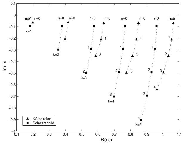
Figure 2: Massless Dirac quasinormal mode frequencies. For the convenience of comparison, double results including KS solution (solid triangle) and Schwarzschild solution (solid square) are given simultaneously.

Table 2: The QN frequencies of null overtones modes ($n=0,k=1$).

$1/2\alpha$	$3th$	$6th$
$0$	$0.176452-0.100109i$	$0.182642-0.094937i$
$0.1$	$0.179189-0.098175i$	$0.184899-0.092152i$
$0.2$	$0.181871-0.096140i$	$0.187179-0.089352i$
$0.4$	$0.187091-0.091667i$	$0.191448-0.083907i$
$0.5$	$0.189632-0.089156i$	$0.193342-0.081265i$
$0.6$	$0.192118-0.086395i$	$0.195055-0.078615i$
$0.8$	$0.196809-0.079810i$	$0.197915-0.072858i$
$1$	$0.200527-0.071134i$	$0.199480-0.065511i$

Table 3: The QN frequencies of null overtones modes ($n=0,k=2$).

$1/2\alpha$	$3th$	$6th$
$0$	$0.378627-0.0965424i$	$0.380069-0.096366i$
$0.1$	$0.381664-0.0949046i$	$0.383040-0.094794i$
$0.2$	$0.384885-0.0931728i$	$0.386218-0.093061i$
$0.4$	$0.391946-0.0893179i$	$0.393230-0.089069i$
$0.5$	$0.395827-0.0871212i$	$0.397087-0.086766i$
$0.6$	$0.399977-0.0846759i$	$0.401200-0.084209i$
$0.8$	$0.409203-0.0786964i$	$0.410286-0.078038i$
$1$	$0.419782-0.0702051i$	$0.420578-0.069468i$

Table 4: The QN frequencies of null overtones modes ($n=0,k=3$).

$1/2\alpha$	$3th$	$6th$
$0$	$0.573685-0.096324i$	$0.574094-0.0963070i$
$0.1$	$0.578089-0.094773i$	$0.578503-0.0947834i$
$0.2$	$0.582754-0.093108i$	$0.583169-0.0931358i$
$0.4$	$0.592999-0.089343i$	$0.593402-0.0893718i$
$0.5$	$0.598659-0.087176i$	$0.599051-0.0871898i$
$0.6$	$0.604747-0.084754i$	$0.605126-0.0847448i$
$0.8$	$0.618500-0.078810i$	$0.618839-0.0787424i$
$1$	$0.635027-0.070293i$	$0.635293-0.0701738i$

For the fixed $\alpha$, we only consider the first five low-lying modes $k=1,\ 2,\ 3,\ 4,\ 5$ with $0\leq n<k$. The results are listed in Table I. The quasinormal mode frequencies for positive $k$ are plotted in Fig.2 which illustrates the real part $Re\omega$ decreases with increasing mode number $n$ for the given angular momentum number $k$. Else, the absolute value of imaginary part $|Im\omega|$ increases as bigger $n$ which indicates higher modes decay faster than the low-lying ones. Comparing with Schwarzschild results (solid quare points), the $Re\omega$ of $\alpha$ is larger than Schwarzschild limit, while the damping rate $|Im\omega|$ is smaller than pure Schwarzschild case.

For the changed $\alpha$, we treat $1/2\alpha$ changed in $[0,1]$ as a whole. Three important kinds low-lying modes: ($k=1,n=0$), ($k=2,n=0$) and ($k=3,n=0$) are listed in Table II, III, and IV, respectively. According these three tables, we plot the real part $Re\omega$ and the imaginary part $Im\omega$ of the third and the sixth order results in Fig.3. Here, it should notice that the horizontal abscissa denotes the value of $1/2\alpha$. We impose the interpretations on these data and draw conclusions from them.

(1) The real part $Re\omega$ increases as bigger $1/2\alpha$ and the absolute value of imaginary part $|Im\omega|$ decreases with increasing $1/2\alpha$, which indicates these QNM could be lived longer.

(2) The gap between the third results and the sixth order ones is visibly displayed in the imaginary part. The real parts of them basically have the same values, except for $k=1$ modes. In general, the average relative magnitudes of the gaps are approximately given as,

$$\bigg{|}\frac{{}^{6th}\text{Im}(\omega)-^{3th}\text{Im}(\omega)}{{}^{3th}\text{Im}(\omega)}\bigg{|} \approx 10\%,$$ (64)

$$\bigg{|}\frac{{}^{6th}\text{Re}(\omega)-^{3th}\text{Re}(\omega)}{{}^{3th}\text{Re}(\omega)}\bigg{|} \approx 0.$$ (65)

Hence, the orders of WKB approxmations have the tremendous bearing on the damping rate, more than on the actual frequency.

Moreover, when horizontal abscissa of Fig.3 approaches Schwarzschild case, namely $1/2\alpha\longrightarrow 0$ (or $\alpha\longrightarrow+\infty$), the real frequencies $Re\omega$ decreases and the damping rate $|Im\omega|$ increases. In another words, the Horava-Lifshitz gravities have the longer lived and more bigger actual frequency than that of usual Schwarzschild case. This specific phenomenon also is observed in the massless scalar field perturbation Konoplya2 ; sbchenqnm .

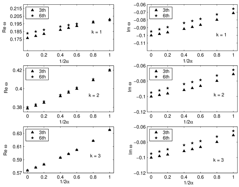
Figure 3: The real parts $Re\omega$ and the imaginary parts $Im\omega$ versus radial $r$ under the third orders (solid triangle) and the sixth orders (solid pentagram) WKB approximations.

V conclusion

In this paper, we have investigated fermions tunneling and perturbation in the IR modified Ho$\check{r}$ava-Lifshitz gravity. We summarize what has been achieved.

(1) For the fermions Hawking radiation, we consider the symmetrical characteristic of spacetime and adopt the action with the form of Eq.(33). Through the decomposition of Dirac Eq.(16), we can get the imaginary part of fermions action which could help us obtain the tunneling probability according to Eq.(42). Then, on the benefit of $\Gamma=\exp(-\beta\omega)$, the tunneling temperature could be given as Eq.(44). So, according to the first law $dM=TdS$, we have a tunneling entropy Eq.(48) naturally. It is interesting that the tunneling Hawking temperature and tunneling entropy are agreement with that obtained by calculating surface gravity.

(2) For the fermions perturbation, we obtain lowly damped quasinormal modes by using the sixth orders WKB approximations, as well as the third orders formulas. In order to get a detail analysis on these obtained quasinormal frequencies, we adopt two kinds of methods: one is to fix the Ho$\check{r}$avaparameter $\alpha$ (fixed $\alpha$) and another is to change $\alpha$ in the range $[0,+\infty]$ (varied $\alpha$).

For the fixed $\alpha$ case, the results turns out that the impact of the Horava-Lifshitz gravity on quasinormal frequencies is quite. This is profoundly manifested in the following ways: the actual frequencies becomes bigger and the damping rate becomes more slower which indicates these lowing modes could be lived longer than that of usual Schwarzschild. This fact also could be explained by the perturbation potential $V_{1}$ Eq.(60) illustrated in Fig.2, which shows the potential contained Horava-Lifshitz gravity (solid lines) is lower than that of Schwarzschild (dotted lines).

For the varied $\alpha$ case, we have calculated numerically three kinds of important lowing modes ($k=1,n=0$), ($k=2,n=0$) and ($k=3,n=1$) by through the third and sixth orders WKB approximations. The result listed in Tables II, III and IV show three facts as follows. (i) With bigger parameter $1/2\alpha$, the real part of frequencies increases and the absolute value of imaginary part decreases which is illustrated by Fig.3. In other words, if parameter $1/2\alpha$ becomes larger, the actual frequency of QNMs will be larger with more longer damping rate. (ii) The real part is not sensitive to the third or the sixth orders WKB approximates. This fact also is illustrated in the left sub-plotted curves in Fig.3, except for some small $1/2\alpha$ modes of $k=1$. (iii) Against the real part, the imaginary part is sensitive to our WKB approximates methods. The gap of the third and the sixth orders results is unchanged basically. This fact also is illustrated in the right sub-plotted curves in Fig.3. In a word, if these specific information could be tested by LIGO, VIRGO, TAMT, GEO600, it will support Ho$\check{r}$ava-Lifshitz gravity forcefully and energetically.

- (1) P. Horava, Quantum Gravity at a Lifshitz Point, Phys. Rev. D 79 (2009) 084008 (2009), [arXiv: 0901.3775]; P. Horava, Spectral Dimension of the Universe in Quantum Gravity at a Lifshitz Point, Phys. Rev. Lett. 102 (2009) 161301, [arXiv: 0902.3657]; P. Horava, Membranes at Quantum Criticality, JHEP 0903 (2009) 020, [arXiv: 0812.4287].
- (2) T. P. Sotiriou, M. Visser and S. Weinfurtner, Phenomenologically viable Lorentz-violating quantum gravity, Phys. Rev. Lett. 102 (2009) 251601, [arXiv: 0904.4464]; M. Visser,Lorentz symmetry breaking as a quantum field theory regulator, Phys. Rev. D80 (2009) 025011, [arXiv: 0902.0590]; R. G. Cai, Y. Liu and Y. W. Sun,On the z = 4 Horava-Lifshitz Gravity, JHEP 0906 (2009) 010, [arXiv: 0904.4104]; B. Chen and Q. G. Huang, Field Theory at a Lifshitz Point, Phys. Lett. B683 (2010) 108-113, [arXiv: 0904.4565]; D. Orlando and S. Reffert, On the Renormalizability of Horava-Lifshitz-type Gravities, Class. Quant. Grav. 26 (2009) 155021, [arXiv: 0905.0301]; R. G. Cai, B. Hu and H. B. Zhang, Dynamical Scalar Degree of Freedom in Horava-Lifshitz Gravity, Phys. Rev. D 80 (2009) 041501, [arXiv: 0905.0255]; T. Nishioka, Horava-Lifshitz Holography, Class. Quant. Grav. 26 (2009) 242001, [arXiv:0905.0473]; M. Li and Y. Pang, A Trouble with Horava-Lifshitz Gravity, JHEP 08 (2009) 015, [arXiv: 0905.2751]; C. Charmousis, G. Niz, A. Padilla and P. M. Saffin, JHEP 0908 (2009) 070,[arXiv: 0905.2579]; T. P. Sotiriou, M. Visser and S. Weinfurtner, Quantum gravity without Lorentz invariance, JHEP 0910 (2009) 033, [arXiv: 0905.2798]; G. Calcagni, Detailed balance in Horava-Lifshitz gravity, Phys. Rev. D81 (2010) 044006, [arXiv: 0905.3740]; D. Blas, O. Pujolas and S. Sibiryakov, On the Extra Mode and Inconsistency of Horava Gravity, JHEP 0910 (2009) 029, [arXiv: 0906.3046]; R. Iengo, J. G. Russo and M. Serone, Renormalization group in Lifshitz-type theories, JHEP 0911 (2009) 020, [arXiv: 0906.3477]; C. Germani, A. Kehagias and K. Sfetsos, JHEP 09 (2009) 060, [arXiv: 0906.1201]; S. Mukohyama, JCAP 09 (2009) 005, [arXiv: 0906.5069]; J. Kluson, Horava-Lifshitz f(R) Gravity, JHEP 0911 (2009) 078, [arXiv: 0907.3566]; N. Afshordi, Cuscuton and low energy limit of Horava-Lifshitz gravity, Phys. Rev. D80 (2009) 081502, [arXiv: 0907.5201]; A. Kobakhidze, Phys. Rev. D 82 (2010) 064011, [arXiv: 0906.5401]; T. Takahashi, J. Soda, Phys. Rev. Lett. 102 (2009) 231301, [arXiv: 0904.0554].
- (3) R. Brandenberger, Matter bounce in Horava-Lifshitz cosmology, Phys. Rev. D 80 (2009) 043516, [arXiv:0904.2835]; Y.S. Piao, Primordial Perturbation in Horava-Lifshitz Cosmology, Phys. Lett. B681 (2009) 1-4, [arXiv:0904.4117]; G. Leon and E. N. Saridakis, Phase-space analysis of Horava-Lifshitz cosmology, JCAP 11 (2009) 006, [arXiv:0909.3571]; M. Chaichian, S. Nojiri, S. D. Odintsov, M. Oksanen and A. Tureanu, Modified F(R) Horava-Lifshitz gravity: a way to accelerating FRW cosmology, Class. Quantum Grav. 27 (2010) 185021, [arXiv:1001.4102]; R. G. Cai and A. Wang, Singularities in Horava-Lifshitz theory, Phys. Lett. B686 (2010) 166-174, [arXiv:1001.0155]; E. Kiritsis and G. Kofinas, Nucl. Phys. B821 (2009) 467-480, [arXiv: 0904.1334]; S. Mukohyama, JCAP 0906, 001 (2009), [arXiv: 0904.2190]; S. Mukohyama,K. Nakayama, F. Takahashi and S. Yokoyama, Phenomenological Aspects of Horava-Lifshitz Cosmology, Phys. Lett. B679 (2009)6-9, [arXiv: 0905.0055]; S. Kalyana Rama, Phys. Rev. D79 (2009) 124031, [arXiv: 0905.0700]; B. Chen, S. Pi and J. Z. Tang, Scale Invariant Power Spectrum in Horava-Lifshitz Cosmology without Matter, JCAP 0908 (2009) 007, [arXiv: 0905.2300]; A. Wang and Y. Wu, JCAP 0907 (2009) 012, [arXiv: 0905.4117]; S. Nojiri and S. D. Odintsov, Covariant renormalizable gravity and its FRW cosmology, Phys. Rev. D81 (2010) 043001, [arXiv: 0905.4213]; A. Wang and R. Maartens, Cosmological perturbations in Horava-Lifshitz theory without detailed balance, Phys. Rev. D81 (2010) 024009, [arXiv: 0907.1748]; T. Kobayashi,Y. Urakawa and M. Yamaguchi, Large scale evolution of the curvature perturbation in Horava-Lifshitz cosmology, JCAP 0911 (2009) 015, [arXiv: 0908.1005]; E. N. Saridakis, Horava-Lifshitz Dark Energy, Eur. Phys. J. C67 (2010) 229-235, [arXiv: 0905.3532]; M. i. Park, A Test of Horava Gravity: The Dark Energy, JCAP 1001(2010)001, [arXiv: 0906.4275].
- (4) R. B. Mann, Lifshitz Topological Black Holes, JHEP 0906 (2009) 075, [arXiv: 0905.1136]; R. G. Cai, L. M. Cao and N. Ohta, Topological Black Holes in Horava-Lifshitz Gravity, Phys. Rev. D 80 (2009) 024003, [arXiv: 0904.3670]; R. G. Cai, L. M. Cao and N. Ohta, Thermodynamics of Black Holes in Horava-Lifshitz Gravity, Phys. Lett. B, 679 (2009) 504-509, [arXiv: 0905.0751]; R. G. Cai, Y. Liu and Y. W. Sun, On the z=4 Horava-Lifshitz Gravity, JHEP 0906 (2009) 010 [arXiv:0904.4104]; H. Lu, J. Mei and C. N. Pope, Phys. Rev. Lett. 103 (2009) 091301 [arXiv:0904.1595]; M. i. Park, The Black Hole and Cosmological Solutions in IR modified Horava Gravity, JHEP 0909 (2009) 123, [arXiv: 0905.4480]; A. N. Aliev, C. Sentrk, Slowly Rotating Black Hole Solutions to Horava-Lifshitz Gravity, Phys. Rev. D82 (2010) 104016, [arXiv:1008.4848]; A. Ghodsi, E. Hatefi, Extremal rotating solutions in Horava Gravity, Phys. Rev. D81(2010) 044016; E. O. Colgain and H. Yavartanoo, Dyonic solution of Horava-Lifshitz Gravity, JHEP 0908 (2009) 021, [arXiv: 0904.4357]; Lee H W, Kim Y W and Myung Y S 2009 Extremal black holes in the Horava-Lifshitz gravity Eur. J. Phys. C 68 255-263 [arXiv:0907.3568].
- (5) A. Kehagias and K. Sfetsos, The black hole and FRW geometries of non-relativistic gravity, Phys. Lett. B 678 (2009) 123-126, [arXiv: 0905.0477].
- (6) E. Kiritsis and G. Kofinas, On Horava-Lifshitz “Black Holes”, JHEP 1001 (2010) 122, [arXiv: 0910.5487].
- (7) D. Capasso and A. P. Polychronakos, General static spherically symmetric solutions in Horava gravity, Phys. Rev. D 81 (2010) 084009, arXiv:0911.1535.
- (8) D. Capasso and A.P. Polychronakos, JHEP 1002:068,2010, [arXiv:0909.5405].
- (9) S. K. Rama, Particle Motion with Horava-Lifshitz type Dispersion Relations, [arXiv:0910.0411].
- (10) A. E. Mosaffa, On Geodesic Motion in Horava-Lifshitz Gravity, [arXiv:1001.0490].
- (11) L. Sindoni, A note on particle kinematics in Horava-Lifshitz scenarios, [arXiv:0910.1329].
- (12) R. A. Konoplya, Towards constraining of the Horava-Lifshitz gravities, Phys. Lett. B679: 499-503, 2009, [arXiv:0905.1523].
- (13) S. B. Chen, J. L. Jing, Strong field gravitational lensing in the deformed Horava-Lifshitz black hole, Phys. Rev. D 80 (2009) 024036 [arXiv: 0905.2055]
- (14) S. B. Chen, J. L. Jing, Quasinormal modes of a black hole in the deformed Horava-Lifshitz gravity, Phys. Lett. B 687(2010) 124-128, [arXiv: 0905.1409].
- (15) J. H. Chen, Y. J. Wang, Timelike Geodesic Motion in Horava-Lifshitz Spacetime, Int. J. Mod. Phys. A 25 2010 1439, [arXiv: 0905.2786].
- (16) T. Harko, Z. Kovacs, F. S. N. Lobo, Testing Horava-Lifshitz gravity using thin accretion disk properties, Phys. Rev. D 80 (2009) 044021, [arXiv: 0907.1449].
- (17) S. Dutta and E. N. Saridakis, Overall observational constraints on the running parameter of Horava-Lifshitz gravity, JCAP 05 (2010) 013, [arXiv:1002.3373]; S. Dutta and E. N. Saridakis, Observational constraints on Horava-Lifshitz cosmology, JCAP 01 (2010) 013, [arXiv:0911.1435]; M. Liu, J. Lu, B. Yu and J Lu, Solar system constraints on asymptotically flat IR modified Horava gravity through light deflection Gen. Rel. Grav. 43, (2010)1401-1415, [arXiv:1010.6149]; L. Iorio, M. L. Ruggiero, Int. J. Mod. Phys. A 25 (2010) 5399-5408, [arXiv:0909.2562]; L. Iorio, M. L. Ruggiero, accepted in The Open Astronomy Journal, [arXiv:0909.5355]; T. Harko, Z. Kovacs, F. S. N. Lobo, Proc. R. Soc.A 467, 2009, 1390-1407, [arXiv:0908.2874]
- (18) Y. S. Myung, Thermodynamics of black holes in the deformed Horava-Lifshitz gravity, Phys. Lett. B 678 (2009) 127 [arXiv:0905.0957]; A. Castillo and A. Larranaga, Entropy for Black Holes in the Deformed Horava-Lifshitz Gravity, [arXiv:0906.4380].
- (19) Y.S. Myung, Entropy of black holes in the deformed Horava-Lifshitz gravity, Phys. Lett. B684 (2010) 158, [Arxiv:0908.4132].
- (20) R. G. Cai and N. Ohta, Horizon Thermodynamics and Gravitational Field Equations in Horava-Lifshitz Gravity, Phys. Rev. D 81(2010) 084061, [arXiv:0910.2307].
- (21) C. Y. Wang and Y. X. Gui, Dirac quasinormal modes of the deformed Horava-Lifshitz black hole spacetime, Astrophys Space Sci (2010) 325: 85 - 91.
- (22) N. Varghese and V. C. Kuriakose, Evolution of electromagnetic and Dirac perturbations around a black hole in Horava gravity, [arXiv:1010.0549].
- (23) D. Y. Chen, H. T. Yang and X. T. Zu, Hawking radiation of black holes in the z = 4 Horava-Lifshitz gravity, Phys. Lett. B681 (2009) 463-468, [arXiv:0910.4821].
- (24) B. F. Schutz and C. M. Will, Astrophys. J., Lett. Ed. 291, L33, 1985.
- (25) S. Iyer and C. M. Will, Black-hole normal modes: A WKB approach. I. Foundations and application of a higher-order WKB analysis of potential-barrier scattering, Phys. Rev. D35 (1987) 3621.
- (26) S. Iyer, Black-hole normal modes: A WKB approach. II. Schwarzschild black holes, Phys. Rev. D35 (1987) 3632.
- (27) R. A. Konoplya, Quasinormal behavior of the D-dimensional Schwarzshild black hole and higher order WKB approach, Phys. Rev. D 68, (2003) 024018, [gr-qc/0303052].
- (28) R. A. Konoplya and E. Abdalla, Phys. Rev. D 71, 084015 (2005) [arXiv:hep-th/0503029]; E. Abdalla, O. P. F. Piedra and J. de Oliveira, arXiv:0810.5489; M. L. Liu, H. Y. Liu and Y. X. Gui, Class. Quant. Grav. 25, 105001 (2008); P. Kanti and R. A. Konoplya, Phys. Rev. D 73, 044002 (2006) [arXiv:hep-th/0512257]; J. F. Chang, J. Huang and Y. G. Shen, Int. J. Theor. Phys. 46, 2617 (2007); H. T. Cho, A. S. Cornell, J. Doukas and W. Naylor, Phys. Rev. D 77, 016004 (2008); Y. Zhang and Y. X. Gui, Class. Quant. Grav. 23, 6141 (2006); R. A. Konoplya, Phys. Lett. B 550, 117 (2002) [arXiv:gr-qc/0210105]; S. Fernando and K. Arnold, Gen. Rel. Grav. 36, 1805 (2004); H. Kodama, R. A. Konoplya and A. Zhidenko, arXiv:0904.2154; H. Ishihara, M. Kimura, R. A. Konoplya, K. Murata, J. Soda and A. Zhidenko, Phys. Rev. D 77, 084019 (2008) [arXiv:0802.0655]; R. A. Konoplya and A. Zhidenko, Phys. Lett. B 644, 186 (2007) [arXiv:gr-qc/0605082];