A numerical study of the overlap probability distribution and its sample-to-sample fluctuations in a mean-field model

Abstract

In this paper we study the fluctuations of the probability distributions of the overlap in mean field spin glasses in the presence of a magnetic field on the De Almeida-Thouless line. We find that there is a large tail in the left part of the distribution that is dominated by the contributions of rare samples. Different techniques are used to examine the data and to stress on different aspects of the contribution of rare samples.

I Introduction

Spin glass models show amazing physical properties. Let us considering for simplicity mean field spin glasses, like the Sherrington-Kirkpatrick model SK , whose solution is given by the hierarchical replica symmetry breaking (RSB) Ansatz mpv ; parisibook2 ; mpv ; G ; TALE . The model is defined by the following Hamiltonian

$$\mathcal{H}[\vec{\sigma}]=-\sum_{i,j}J_{ij}\sigma_{i}\sigma_{j}\;,$$ (1)

where $\sigma_{i}=\pm 1$ are $N$ Ising spins and the $J_{ij}$ are quenched random couplings with zero mean and variance $1/N$.

For each sample $\mathcal{J}$, that is for a choice of the quenched random couplings, one can compute the probability distribution function of the overlap, $q=\sum_{i=1}^{N}\sigma_{i}\tau_{i}/N$, between two replicas $\vec{\sigma}$ and $\vec{\tau}$ subject to the same Hamiltonian (1): we call $P_{\mathcal{J}}(q)$ such a probability distribution.

In the SK model the order parameter in the thermodynamical limit is given by a function $q(x):[0,1]\to[0,1]$, related to the probability distribution $P(q)$ of finding two replicas at an overlap $q$, where $P(q)$ is defined as

$$P(q)=\overline{P_{\mathcal{J}}(q)}\;,$$

and the overline represents the average over the samples $\mathcal{J}$’s.

The overlap distribution $P_{\mathcal{J}}(q)$ strongly fluctuates from sample to sample. In the low temperature spin glass phase ($T<T_{c}$), these distributions are not self-averaging, that is the typical $P_{\mathcal{J}}(q)$ is very different from the disorder averaged distribution $P(q)$, even in thermodynamical limit. The size of these fluctuations in the SK model can be quantified by using the Ghirlanda-Guerra relations RUELLETREE ; mpv ; GG ; AI ; SOL ; the simplest identity is

$$\overline{P_{\mathcal{J}}(q)P_{\mathcal{J}}(q^{\prime})}-\overline{P_{\mathcal{J}}(q)}\;\overline{P_{\mathcal{J}}(q^{\prime})}=\frac{1}{3}\Big{[}\delta(q-q^{\prime})-P(q)\Big{]}P(q^{\prime})\;,$$

and the r.h.s. is non null as soon as the $P(q)$ is not a delta function, i.e. when replica symmetry is broken.

These large sample-to-sample fluctuations play a very relevant role in numerical simulations, since they require a huge number of samples to obtain reliable measurements in the low temperature phase of spin glass models, and they may produce finite size effects that vanish very slowly, increasing system size.

In the present paper we study overlap distributions in a mean-field spin glass model, defined on a Bethe lattice of fixed degree, in the presence of an external field. We focus on the data measured at the critical temperature $T_{c}$, such that the mean overlap distribution in the thermodynamical limit is a delta function, $P(q)=\delta(q-q_{0})$. This choice has two main advantages:

• we know analytically the value of $T_{c}$ and $q_{0}$, by solving the model with the cavity method, and this allows us to better study deviation from the thermodynamical limit (i.e., finite size effects);

• the system is critical and so it shows very large sample to sample fluctuations.

For any temperature different from $T_{c}$ one of the two above statement would be false, thus making our study less interesting. Moreover the presence of the external field breaks the global spin inversion symmetry and implies that overlaps are non-negative in the thermodynamical limit: however it is well known that a large tail in the negative overlap region is present in systems of finite size and its origin needs to be clarified.

II The model and the numerical simulations

We study an Ising spin glass model defined on a Bethe lattice of fixed connectivity $c=4$ (i.e., a random regular graph of fixed degree $c=4$). The Hamiltonian is

$$\mathcal{H}=-\sum_{<ij>}J_{ij}\sigma_{i}\sigma_{j}-H\sum_{i}\sigma_{i}\;,$$ (2)

where $\sigma_{i}=\pm 1$ are $N$ Ising spins, the couplings $J_{ij}=\pm 1$ (with equal probability) are quenched random variables and the sum runs over all pairs of neighboring vertices in the graph. We use a constant external field $H>0$. For not very small connectivity Ising spin glasses on a Bethe lattice share many properties with the Sherrrington-Kirkpatrick model VB ; BETHE : in the limit $c\to\infty$ we recover the Sherrington Kirkpatrick model, and the $1/c$ corrections are well under control ParisiTria .

We construct the random regular graph in the following way: we attach $c$ legs to each vertex and then we recursively join a pair of legs, forming a link, until no legs are left or a dead end is reached (this may happen because we avoid self-linking of a vertex and double-linking between the same pair of vertices); if a dead end is reached, the whole construction is started from scratch.

Similarly to the SK model, the model (2) has a continuous spin glass phase transition at a critical temperature $T_{c}$ which depends both on the value of $c$ and $H$. At variance with the SK model, the critical line in the $(T,H)$ plane does not diverge when $T\to 0$, but rather reaches a finite value $H_{c}$ (see Fig. 1). This is due to the finite number of neighbors each spin has on a random graph of finite mean degree (while this number is divergent with the system size in the SK model). In this sense the present model is closer to finite dimensional models than the SK model is.

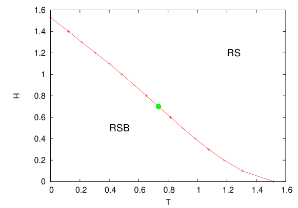
Figure 1: Phase diagram in the temperature–field plane for the $J=\pm 1$ spin glass model defined on a Bethe lattice of fixed degree $c=4$. In this work we report data collected at the critical point marked by a big dot.

The replica symmetric (RS) phase of model (2) can be solved analytically by the cavity method BETHE . In particular one can find the boundary of the RS phase, beyond which the model solution spontaneously breaks the replica symmetry PaPaRa ; TaRiKa . In Fig. 1 we show such a critical line in the $(T,H)$ plane for the model with fixed degree $c=4$. The high temperature and/or high field region is replica symmetric, while a breaking of the replica symmetry is required in the low temperature and low field region. We have checked that the phase boundary behaves like $H_{c}(T)\propto(T-T_{c})^{3/2}$ close to zero-field critical point $T_{c}$, and the exponent is the same one found in the SK model.

We have carried our Monte Carlo simulations at the point marked with a big dot in Fig. 1, that is $H=0.7$ and $T=0.73536$. The uncertainty on the critical temperature for $H=0.7$ is $10^{-5}$. At that point the value of the thermodynamical overlap is $q_{0}=0.67658(1)$. Please notice that we have chosen a rather large value of the external field, which is roughly half of the largest critical field value $H_{c}(T=0)\simeq 1.53$, in order to avoid crossover effects that could be due to the vicinity of the zero-field critical point.

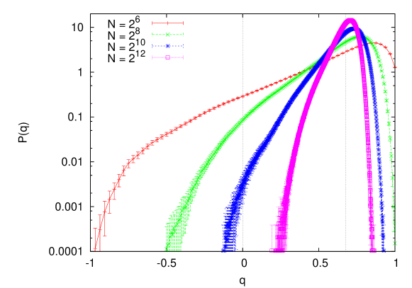
Figure 2: Disorder averaged overlap probability distributions $P(q)$ show an exponential tail for $q<q_{0}$.

Monte Carlo simulations have been performed by using the Metropolis algorithm and the parallel tempering method: we used 20 temperatures equally spaced between $T_{max}=2.0$ and $T_{c}=0.73536$, and we attempted the swap of configurations at nearest temperatures every 30 Monte Carlo sweeps (MCS). Each sample (of any size) has been thermalized for $2^{24}$ MCS and then 1024 measurements have been taken during other $2^{26}$ MCS: so there are $2^{16}$ MCS between two successive measurements and we have checked this number to be larger than the autocorrelation time. We study systems of sizes ranging from $N=2^{6}$ to $N=2^{14}$, with a number of samples ranging from 5120 for $N=2^{6}$ to 1280 for $N=2^{14}$. We are going to present only the data for sizes $N\leq 2^{12}$ for which we have simulated at least 2560 samples; indeed the data for $N=2^{13}$ and $N=2^{14}$ are more noisy (due to the limited number of samples), moreover we fear that some samples may not be perfectly thermalized even after $2^{26}$ MCS. By restricting to $N\leq 2^{12}$ we are fully confident about the numerical data.

III Results

We start by showing in Fig. 2 the disorder averaged $P(q)$ for different sizes. The exponential tail on the left side is evident from the plot (which is on a logarithmic scale): this tail goes far in the negative overlap region for small sizes. In the following we are going to show that this exponential tail is not a feature of typical samples, but it is completely due to very rare and atypical samples.

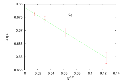
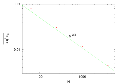
Figure 3: Mean (left) and variance (right) of $P(q)$. A naive analysis would predict an asymptotic value for $\langle q\rangle$ larger than $q_{0}$ and finite size corrections decaying faster than the $N^{-1/3}$ expected behavior. The variance decays roughly as the expected $N^{-2/3}$ law.

The vertical line at $q=q_{0}$ in Fig. 2 marks the location of the delta peak in the thermodynamical limit. By looking at the mean and the variance of $P(q)$ we have checked how finite size effects decay to zero. We see in Fig. 3 that while $\overline{\langle q^{2}\rangle}_{c}$ decays in a way compatible with the expected behavior $N^{-2/3}$ (the discrepancy can be well explained in terms of small scaling corrections), the mean overlap $\overline{\langle q\rangle}$ shows finite size corrections proportional to $N^{-1/2}$ (instead of the expected $N^{-1/3}$) and seems to extrapolate to a thermodynamical limit different from $q_{0}$. This means that a naive extrapolation to the thermodynamical limit would produce a wrong estimate of $q_{0}$. The most probable explanation is that finite size corrections of order $N^{-1/2}$ have a much larger coefficient than those of order $N^{-1/3}$ and then much larger sizes are needed to observe the asymptotic behavior.

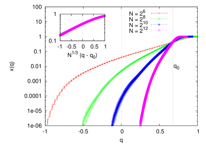
Figure 4: The integrated probability distribution $x(q)$ averaged over the disorder. The value of $q_{0}$ can be well determined by the crossing point of data set in the main panel. The inset show the scaling function $x(N^{1/3}(q-q_{0}))$.

A much better way to estimate $q_{0}$ from the disorder averaged data seems to be the analysis of the overlap integrated probability function

$$x(q)\equiv\int_{-1}^{q}P(q^{\prime})dq^{\prime}\;.$$

This variable has been used for studying the behavior of three dimensional systems at zero magnetic field MaPaRu ; Janus5 . The results are shown in Fig. 4. In the main panel we see again the exponential tail on the left side, but the crossing point of the functions $x(q)$ estimates with a high accuracy the right value for $q_{0}$. In the present case all the crossing points for the sizes shown are within a distance less than $10^{-3}$ from the thermodynamical value and converge to it according to the $N^{-1/3}$ law. In the inset of Fig. 4 we show that $x(q)$ data perfectly collapse when plotted as a function of the scaling variable $N^{1/3}(q-q_{0})$.

Let us now turn to the study of sample-to-sample fluctuations. We want to convince the reader that the exponential tail is not a feature of typical samples: actually not even a feature of the vast majority of samples, that show roughly Gaussian (or even steeper) tails in their $P_{\mathcal{J}}(q)$. The exponential tail is produced by the integration of the secondary peak that atypical samples have at an overlap value much smaller than $q_{0}$.

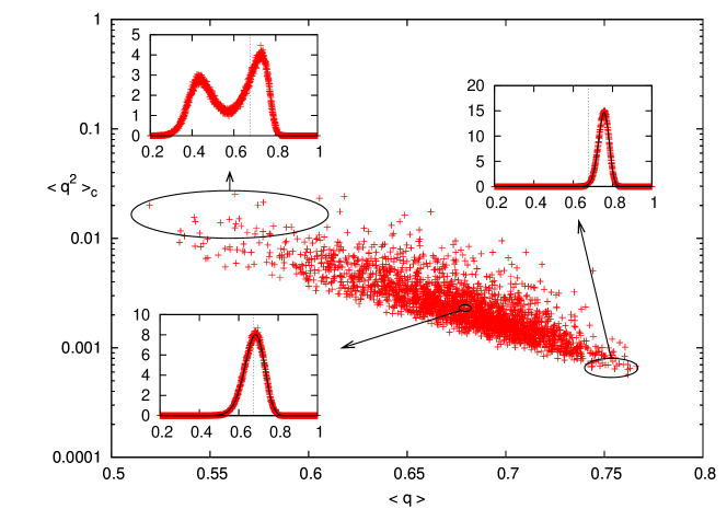
Figure 5: Mean and variance of the 2560 samples of size $N=2^{12}$. Insets show the overlap probability distribution averaged over a small fraction, $1/128$, of samples (those in the corresponding circle). Solid curves in the insets are Gaussian fits to the data (see text for details).

Extracting typical and atypical shapes of the $P_{\mathcal{J}}(q)$ from thousands of samples is not a straightforward job. We follow the simplest procedure based on the analysis of the first two moments. In the main panel of Fig. 5 we show the mean and the variance of the 2560 samples of size $2^{12}$. The three insets in Fig. 5 show the averages over 20 $P_{\mathcal{J}}(q)$ chosen from typical samples (lower inset) or from atypical samples, either much broader or much narrower than typical (upper insets). In every inset we also draw a dashed vertical line to mark the location of $q_{0}$.

We notice that there exist a large difference between typical an atypical samples, both quantitatively and qualitatively (especially for the atypical samples showing a double peak structure). However the very different shapes can be roughly accounted for by considering an effective external field different from the one ($H=0.7$ in the present case) appearing in the Hamiltonian: in the atypical samples shown in the upper right inset this effective field is larger than $H$ and thus the overlap distribution is narrower and centered on a value greater than $q_{0}$, while the atypical samples shown in the upper left inset look like if they were below the critical line, i.e. with a field smaller than $H$.

Since samples with different effective fields will have different critical temperatures, it is possible that the main source of sample-to-sample fluctuations can be well described by a random temperature (or field) term in the effective Hamiltonian as in the case of ferromagnets in random magnetic field Sou ; PaSou ; PaPiSou .

It is also worth noticing that the tails of the distributions shown in the insets of Fig. 5 are Gaussian or even steeper, as expected FraPaVi . Indeed, the interpolating curves superimposed to the bimodal distributions (lower left and upper right insets) have been obtained by assuming $q=\tanh(h)$ with a Gaussian distributed local field $h$. The non-linear transformation is necessary (and sufficient) to take into account the small skewness of the distributions.

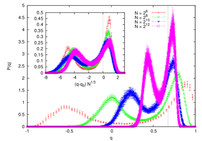
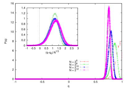
Figure 6: Most atypical distributions, averaged over a fraction $1/128$ of samples: those with the largest (left) and smallest (right) variance. By varying the system size they roughly preserve the shape and get shrunk according to the scaling $q-q_{0}\sim N^{-1/3}$ (see insets).

In Fig. 5 we have presented data only for size $N=2^{12}$, but a natural question is how sample-to-sample fluctuations vary with the system size. We have found that by increasing the system size the distribution of the moments shrinks towards the thermodynamical limits ($\langle q\rangle=q_{0}$ and $\langle q^{2}\rangle_{c}=0$) with the expected $N^{-1/3}$ scaling behavior. However it is not true that all samples become typical in the thermodynamical limit. In other words the fraction of atypical samples (e.g. those with a bimodal distribution) remains roughly constant. In Fig. 6 we show the average $P(q)$ computed on a small fraction (1/128) of samples, those most atypical, i.e. those corresponding to upper insets in Fig. 5. We notice that, by varying the size, the shape is more or less preserved and the main effect is an overall shrink of the distribution. The insets in Fig. 6 show that this shrinking is consistent with the scaling law $q-q_{0}\sim O(N^{-1/3})$ that holds at criticality.

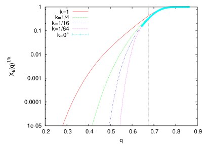
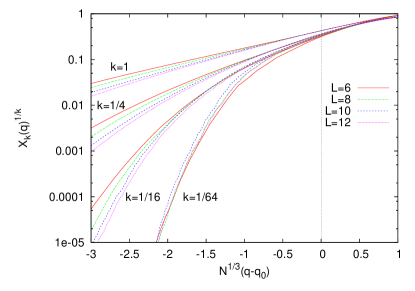
Figure 7: Left: Small $k$ moments of $X_{\mathcal{J}}(q)$ measured in systems of size $N=2^{12}$ show a decay faster than exponential for $q\ll q_{0}$. Right: Systems of different sizes show the same behavior, once the overlap is rescaled accordingly.

Given that neither typical nor atypical distributions have an exponential tail, the only possible explanation is that such a tail is generated by the secondary peak of broader distributions when averaging over the samples. We are going to provide quantitative evidence for this by looking at the integrated probabilities

$$X_{\mathcal{J}}(q)\equiv\int_{-1}^{q}P_{\mathcal{J}}(q^{\prime})dq^{\prime}\;.$$

Let us define the moments of the random variable $X_{\mathcal{J}}$ as

$$X_{k}(q)\equiv\overline{X_{\mathcal{J}}(q)^{k}}\;.$$

Remind that $X_{1}(q)=x(q)$ is plotted in Fig. 4 and shows an exponential tail. However in the region $q\ll q_{0}$ the average $X_{1}(q)$ is dominated by rare samples, while the vast majority of samples has a very small value $X_{\mathcal{J}}(q)\ll X_{1}(q)$ and do not contribute to $X_{1}(q)$.

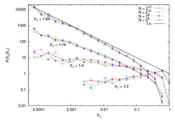
Figure 8: Histograms of $X_{\mathcal{J}}$ at fixed values of $X_{1}$. The data for $X_{1}=1/64$ has been multiplied by 10 in order to improve readability.

In order to extract the behavior of typical samples one should average the random variable $\log(X_{\mathcal{J}}(q))$. However for $q\ll q_{0}$ there are samples with $X_{\mathcal{J}}(q)=0$ and a straightforward computation of $\overline{\log[X_{\mathcal{J}}(q)]}$ is not possible. However, by noticing that

$$\overline{\log[X_{\mathcal{J}}(q)]}=\lim_{k\to 0}\log\left[X_{k}(q)^{1/k}\right]\;,$$

it is possible to observe the behavior of typical samples by choosing $0<k\ll 1$. In Fig. 7 (left) we plot $X_{k}(q)$ for $k=1,1/4,1/16,1/64$ and we clearly see how the exponential tail for $k=1$ becomes a Gaussian (or even steeper) decay for $k\ll 1$. Moreover this behavior is very well conserved by varying the system size: in Fig. 7 (right) we plot the same averages, $X_{1}$ to $X_{1/64}$, as a function of the scaling variables $N^{1/3}(q-q_{0})$ and we see that the data collapse (which is very good for $q\simeq q_{0}$) remains a reasonable approximation in the entire $q$ range. This observation suggests that the entire distribution of the random variable $X_{\mathcal{J}}(q)$ mainly depends on the scaling variable $N^{1/3}(q-q_{0})$, or equivalently on the first moment $X_{1}$. This can be checked in Fig. 8 where we plot the distribution of $X_{\mathcal{J}}$ at some fixed value of $X_{1}$ for several system sizes. Please note that the data for $X_{1}=1/64$ have been multiplied by a factor 10 in order to avoid overlaps with other data set and improve readability.

By commenting Fig. 8 we can finally draw the main conclusions of this analysis. First of all, the good data collapse for the probability distribution of $X_{\mathcal{J}}$ at fixed value of $X_{1}$ is a strong indication that we have measured large enough systems in the asymptotic scaling regime. Moreover we see that for $X_{1}=1/2>x(q_{0})\simeq 0.429$ the distribution of $X_{\mathcal{J}}$ has a maximum close to $X_{1}$, that is the mean value is representative of typical samples behavior. On the contrary, for $X_{1}<x(q_{0})$, the distributions of $X_{\mathcal{J}}$ have their maxima at $X_{\mathcal{J}}\simeq 0$ and the mean value is not representative of typical values. In particular we observe that for very small values of $X_{1}$ the distribution of $X_{\mathcal{J}}$ develops a power law divergence $1/X_{\mathcal{J}}$ for $X_{\mathcal{J}}\to 0$.

IV Conclusions

In this paper we have seen that on the De Almeida-Thouless line the left tail of the distribution of $P(q)$ is dominated by rare samples. The presence of a left tail in the probability is quite an annoying phenomenon that is present also in the Sherrington-Kirpatrick model BiCo and in finite dimensional models LePaRiRu , both at the phase transition point and below the transition. This tail is particularly bothering at not too large magnetic field, because it extends in the region of negative $q$. We think that understanding the origin of this tail may be useful in future analysis of the finite dimensional simulations.

It would be very useful to derive the results on this paper in an analytic way extending the techniques of FraPaVi . Indeed in that paper the computation of the tail was done for the typical samples and we have to modify it in order to compute the tail of the average over the samples. We believe that this is a feasible task.

References

- (1) D. Sherrington and S. Kirkpatrick, Phys. Rev. Lett. 35, 1792 (1975).
- (2) E. Marinari, G. Parisi, F. Ricci-Tersenghi, J. Ruiz-Lorenzo, F. Zuliani J. Stat. Phys. 98, 973 (2000).
- (3) M. Mézard, G. Parisi and M.A. Virasoro, Spin glass theory and beyond, World Scientific (Singapore 1987).
- (4) G.Parisi, Field Theory, Disorder and Simulations, World Scientific, (Singapore 1992).
- (5) F. Guerra, Comm. Math. Phys. 233, 1 (2003).
- (6) M. Talagrand, C.R.A.S. 337, 111 (2003); Ann. Math. 163, 221 (2006).
- (7) D. Ruelle, Comm. Math. Phys. 48, 351 (1988).
- (8) S. Ghirlanda and F. Guerra, J. Phys. A: Math. Gen. 31, 9149 (1998).
- (9) M. Aizenman and P. Contucci, J. Stat. Phys. 92, 765 (1998).
- (10) G. Parisi, Int. J. Mod. Phys. B 18, 733 (2004).
- (11) L. Viana and A.J. Bray, J. Phys. C 18, 3037 (1985).
- (12) M. Mézard, G. Parisi, Eur. Phys. J. B 20, 217 (2001).
- (13) G. Parisi and F. Tria, Eur. Phys. J. B 30, 533 (2002).
- (14) A. Pagnani, G. Parisi and M. Ratiéville, Phys. Rev. E 68, 046706 (2003).
- (15) H. Takahashi, F. Ricci-Tersenghi, and Y. Kabashima, Phys. Rev. B 81, 174407 (2010).
- (16) E. Marinari, G. Parisi, J. J. Ruiz-Lorenzo, Phys. Rev. B 58, 14852 (1998).
- (17) R. Alvarez Ba os, A. Cruz, L. A. Fernandez, J. M. Gil-Narvion, A. Gordillo-Guerrero, M. Guidetti, D. I iguez, A. Maiorano, F. Mantovani, E. Marinari, V. Martin-Mayor, J. Monforte-Garcia, A. Mu oz-Sudupe, D. Navarro, G. Parisi, S. Perez-Gaviro, F. Ricci-Tersenghi, J. J. Ruiz-Lorenzo, S. F. Schifano, B. Seoane, A. Tarancon, R. Tripiccione, D. Yllanes, Sample-to-sample fluctuations of the overlap distributions in the three-dimensional Edwards-Anderson spin glass, arXiv:1107.5772 (2011).
- (18) N. Sourlas Universality in Random Systems: the case of the 3-d Random Field Ising model, arxiv:cond-mat/9810231 (1998).
- (19) G. Parisi and N. Sourlas, Phys. Rev. Lett. 89, 257204 (2002).
- (20) G. Parisi, M. Picco and N. Sourlas, Europhys. Lett. 66, 465 (2004).
- (21) S. Franz, G. Parisi and M. Virasoro, J. Phys. I France 2, 1869 (1992).
- (22) A. Billoire, S. Franz and E. Marinari, J. Phys. A 36 15 (2003).
- (23) A. Billoire and B. Coluzzi, Phys. Rev. E 67, 036108 (2003), Phys. Rev. E 68, 026131 (2003).
- (24) L. Leuzzi, G. Parisi, F. Ricci-Tersenghi, and J. J. Ruiz-Lorenzo, Phys. Rev. Lett. 103, 267201 (2009).