A Formalism for Scattering of Complex Composite Structures. 1 Applications to Branched Structures of Asymmetric Sub-Units.

Abstract

We present a formalism for the scattering of an arbitrary linear or acyclic branched structure build by joining mutually non-interacting arbitrary functional sub-units. The formalism consists of three equations expressing the structural scattering in terms of three equations expressing the sub-unit scattering. The structural scattering expressions allows a composite structures to be used as sub-units within the formalism itself. This allows the scattering expressions for complex hierarchical structures to be derived with great ease. The formalism is furthermore generic in the sense that the scattering due to structural connectivity is completely decoupled from internal structure of the sub-units. This allows sub-units to be replaced by more complex structures. We illustrate the physical interpretation of the formalism diagrammatically. By applying a self-consistency requirement we derive the pair distributions of an ideal flexible polymer sub-unit. We illustrate the formalism by deriving generic scattering expressions for branched structures such as stars, pom-poms, bottle-brushes, and dendrimers build out of asymmetric two-functional sub-units.

I Introduction

Scattering techniques, such as light scattering, small-angle neutron or X-ray scattering (LS, SANS and SAXS, respectively) are ideally suited for probing the structure of suspensions of macromolecules, colloidal particles, and self-assembled structures, see e.g. Guinier and Fournet (1955); Higgins and Benoit (1994); Lindner and Zemb (2002). To extract as much structural information as possible, the data obtained from a scattering experiment need to be analyzed via extensive modeling, since scattering techniques do not provide a real space picture or representation of the structure. A prerequisite for the data modeling is the availability of a large number of expressions for the form and structure factors corresponding to various geometric models for the structures. Fitting such expressions to the measured scattering data allows the structural parameters to be extracted in an reliable and accurate manner. Fortunately, scattering expressions have been derived for a large number of model structures see e.g. Pedersen (2002). Significant efforts are often involved when deducing new scattering expressions for the analysis of complex structures. Hence, it is of great importance to have a simple formalism for how to combine existing model structures to generate new scattering expressions for new and more complex structures.

In the case of regular polymer structures, quite a few expressions have been derived for example linear chainsDebye (1947), block copolymersLeibler (1980); Leibler and Benoit (1981), starsBenoit (1953); Berry and Orofino (1964); Burchard (1974), dendrimersBurchard et al. (1984); Hammouda (1992); Boris and Rubinstein (1996), and bottle-brush polymersCasassa and Berry (1966); Pedersen (1997). These expressions has been derived assuming that a specific structure has been build out of linear polymer sub-units. The polymer sub-units are assumed to be non-interacting and described by Gaussian chain statistics. With these assumptions, the scattering from a structure can be deduced from the contour length distribution separating pairs of scatterers within a structure. The challenge is then how to derive the contour length distribution for a given structure.

The scattering from more complex heterogeneous structures such as block-copolymer micellesPedersen and Gerstenberg (1996); Pedersen and Svaneborg (2002) can also be derived. Here one has to take into account that the scattering length density and structures of the core and corona chains, respectively, are different. The micellar scattering has contributions from pairs of scatterers in the core, pairs of scatterers in the corona and core, and pairs of scatterers on the same and different chains in the corona. The scattering is derived by calculating all the pair-distances between the scatterers, taking their connectivity and structure into account, and neglecting interactions between the core and the corona chains. The micelle models has been generalized to include a radial rod-like connector between the corona chains and the core surface to account for chain stretching close to the coreSvaneborg and Pedersen (2000) and has also been generalized to describe various core geometriesPedersen (2000).

The situation becomes significantly more complex when taking the intra molecular interactions such as excluded volume or Coulombic interactions into account. These can be studied analytically by conformational-space renormalization group theory see e.g. de Gennes (1979); Freed (1983a, b, 1987); Biswas and Cherayil (1994). An alternative is to perform computer simulations of molecular models. Computer simulations have, for instance, been applied to study the effects of excluded volume interactions in flexible polymersWittkop et al. (1996), semi-flexible polymersPedersen and Schurtenberger (1996, 1999), bottle-brush polymersElli et al. (2004); Yethiraj (2006); Hsu et al. (2008) micellesPedersen and Gerstenberg (1996); Svaneborg and Pedersen (2001, 2002) and star-burst polymersCarl (1996); Timoshenko et al. (2002); Ballauff and Likos (2004); Echenique et al. (2009). Common for renormalization group theory and computer simulations are that they can only be applied to specific structures, and there are no general way to generalize the scattering form factors to predict the scattering from related structures.

In the dilute solution case, suspended structures will on average be far apart and their mutual interactions can be disregarded. Then the scattering is given by the form factor of the single structures. At higher concentrations the mutual interaction between structures gives rise to spatial correlations, that can be observed as the emergence of a structure factor peak effects in the scattering spectrum. Various approaches such as the Random-Phase ApproximationBenoit and Benmouna (1984) or sophisticated liquid-state theories such as the PRISM formalismSchweizer and Curro (1987, 1994) can predict concentration effects on the scattering. However, both of these approaches require the form factor as an input.

We present a formalism for predicting the scattering from general linear and branched structures composed of mixtures of heterogeneous sub-units with arbitrary functionality. The formalism is exact for sub-units that are mutually non-interacting, for links that are completely flexible and applies to structures that do not contain loops. No assumptions are made regarding the internal structure or interactions within the sub-units. The central idea of regarding a structure as composed by non-interacting sub-units or blocks describing have been utilized previously by D. J. Read and H. Benoit et al.Benoit and Hadziioannou (1988); Read (1998); Teixeira et al. (2007).

Here we derive the formalism for sub-units with arbitrary functionality, and derive the terms required to use whole structures as sub-units within the formalism itself. We illustrate the formalism with a diagrammatic interpretation, that establishes a direct connection between a general branched structure and the scattering expressions characterizing that structure. In particular, we derive the scattering that results when two known structures are joined by a common point. We also illustrate the formalism by deriving the scattering expressions for an $ABC$ structures build out of arbitrary sub-units, and for an $AB$ structure, chains, alternating chains, stars, chains of stars, pompoms and dendrimers build out of asymmetric two-functional units.

In the present paper, we derive the general formalism, and illustrate it using complex structures composed of a single sub-unit type, while in an accompanying papercs_ , we will review expressions for a variety of sub-units and derive scattering expressions for simple structures focusing on that the different ways sub-units can be joined together. Taken together the two papers allow the scattering from a large variety of heterogeneous branched structures to be derived with great ease. When modeling an experimental small-angle scattering spectrum, one typically starts with a geometric model from which a form factor can be derived. This process can be quite laborious and has to be repeated until the model describes the experimental data. Our vision is to build model structures by joining together well defined sub-units together until we obtain a good fit to the experimental scattering data. The present formalism is a first step in this direction as it ’automates’ the process of deducing the form factor of a structure. Furthermore, within the present formalism it is trivial to change the connectivity of the structure, add new sub-units, or replace existing sub-units by sub-units with a different structure.

The paper is structured as follows: In Sect. II the formalism is presented, and the diagrammatic interpretation of the physics is illustrated with a general $ABC$ structure in sect. III. We introduce the special case of asymmetric two-functional sub-units in sect. IV. Polymers comprise the most important sub-units, and in sect. V we derive the scattering expressions of a polymeric sub-unit. To illustrate the formalism in the case of two-functional sub-units we derive the scattering expressions for chains (sect. VI), stars and chains of stars and pom-poms (sect. VIII) and dendrimers (sect. IX). Finally, we conclude the paper in sect. X.

II Theory

The present theory pertains to the small-angle scattering from arbitrary sub-units and how to efficiently calculate the scattering spectra of complex hierarchical structures, that can be build by joining such sub-units at common points denoted vertices. Assume that the $I$’th sub-unit is composed of point-like scatterers, where the $j$’th scatterer in the sub-unit is located at a position ${\bf r}_{Ij}$ and has excess scattering length $b_{Ij}$. The scattering length describes the interaction between a scatterer and the incident radiation, which could be light, X-rays or neutrons depending on the nature of the scattering experiment. Let ${\bf R}_{I\alpha}$ denote the position of the $\alpha$’th reference point associated with the $I$’th sub-unit. A reference point is a potential point for connecting the sub-unit to other sub-units. A single sub-unit can have an arbitrary number of such reference points associated with it. While the scattering sites are real physical entities, the reference points are just practical handles that we imagine are fixed somewhere on the scattering sub-unit. If the sub-unit is a polymer, then a natural choice would for instance be to have the two ends as reference points. Once two or more sub-units are connected at the same reference point, we refer to it as a vertex in the resulting structure, e.g. if sub-units $I$ and $J$ are joined at reference point $\alpha$ then ${\bf R}_{I\alpha}={\bf R}_{J\alpha}$ denotes the same location in space and vertex in the structure. Here and in the following capital letters refers to sub-units, lower case letters refers to scatterers inside a sub-unit, and Greek letters refers to vertices and reference points.

Small-angle scattering experiments measure pair-correlation functions. For a given sub-unit $I$, we can define three types of pair-correlation functions: Between all pairs of scattering sites, between all scattering sites and a specified reference point $\alpha$, and between two specified reference points $\alpha$ and $\omega$, respectively. These are most conveniently stated in the form of the Fourier transforms

$$F_{I}(q)=\left(\beta_{I}\right)^{-2}\left\langle\sum_{j,k}b_{Ij}b_{Ik}e^{i{\bf q}\cdot({\bf r}_{Ij}-{\bf r}_{Ik})}\right\rangle_{I},$$ (1)

$$A_{I\alpha}(q)=\left(\beta_{I}\right)^{-1}\left\langle\sum_{j}b_{Ij}e^{i{\bf q}\cdot({\bf r}_{Ij}-{\bf R}_{Ij})}\right\rangle_{I},$$ (2)

and

$$\Psi_{I\alpha\omega}(q)=\left\langle e^{i{\bf q}\cdot({\bf R}_{I\alpha}-{\bf R}_{I\omega})}\right\rangle_{I}.$$ (3)

The parameter $q$ is the modulus of the scattering vector and it is defined by the angle between the incident and scattered beam and the wave length of the radiation. In the following, we will denote $F_{I}$ the form factor, $A_{I\alpha}$ the form factor amplitude relative to the reference point $\alpha,$ $\Psi_{I\alpha\omega}$ the phase factor between reference points $\alpha$ and $\omega$, and $\beta_{I}=\sum_{j}b_{Ij}$ the excess scattering length of the $I$’th sub-unit. The $\langle\text{$\cdots$}\rangle_{I}$ averages are over internal conformations and orientations of the $I$´th sub-unit. Due to the orientational average, the Fourier transformed pair-correlation functions only depend on the magnitude of the momentum transfer $q$. Here and in the rest of the paper, the form factor, form factor amplitudes, and phase factors are normalized to unity in the limit $q\rightarrow 0$.

The physical significance of the three scattering terms are as follows. The form factor determines the scattering intensity one obtains from a dilute solution of a single type of sub-units. Here and in the following we neglect the spatial correlations that occur at high concentrations. The scattering intensity at a certain momentum transfer $q$ is determined from the all the interfering waves scattered from the scattering sites in the sub-unit. In a given conformation of the $I$’th sub-unit, two sites $j$ and $k$ contribute interfering waves with a phase shift $i{\bf q}\cdot({\bf r}_{Ij}-{\bf r}_{Ik})$ and an amplitude given by scattering strength $b_{Ij}b_{Ik}$ which is determined by the excess scattering lengths of the two sites compared to the scattering length density of the solution. The resulting intensity is averaged over all conformations and orientations of the sub-unit to produce $F_{I}(q)$.

The form factor amplitude is the total amplitude of the waves scattered from the scattering sites in the sub-unit with the phase shift $i{\bf q}\cdot({\bf r}_{Ij}-{\bf R}_{I\alpha})$ measured relative to a specific reference point and a scattering strength $b_{Ij}$. The resulting amplitude is averaged over all conformations and orientations to produce $A_{I\alpha}(q)$. The phase factor measures the average phase difference between two reference points averaged over sub-unit conformations and orientations. In the special case where the distance is fixed, then the phase factor is given by $\Psi_{I\alpha\omega}(q)=\sin(q|{\bf R}_{\alpha}-{\bf R}_{\omega}|)/(q|{\bf R}_{\alpha}-{\bf R}_{\omega}|)$. Neither the form factor amplitude nor the phase factor can be measured directly for single sub-units in dilution, but their contributions to complex structures can be inferred using contrast variation variation techniques.

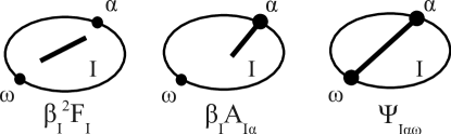
Figure 1: Diagrams and symbols for the form factor, form factor amplitude relative to the reference point $\alpha$ and phase factor between reference points $\alpha$ and $\omega$. The $\beta_{I}$ prefactor is the total excess scattering length of the $I$’th sub-unit.

The form factor, form factor amplitude and phase factor can be regarded as propagators of correlation analogous to Feynman diagrams from quantum field theory or Mayer cluster diagrams from liquid state theory, see e.g. Itzykson and Zuber (1980); Hansen and McDonald (2006). In fig. 1, we diagrammatically represent the sub-unit as an ellipse, where the scattering sites are associated with the inside the ellipse, and reference points are associated with the circumference of the ellipse. The form factor is shown as a line inside the sub-unit, because it represents the sub-units site-to-site pair-correlation function which propagates position information between unspecified pairs of scattering sites inside the sub-unit. The form factor amplitude is shown as a line between a reference point and the sub-unit interior, because it represents the site-to-reference point pair-correlation function which propagates position information between scattering sites in the sub-unit and the specified reference point. Finally, the phase factor is shown as a straight line between to reference points, because it represents the reference point-to-reference point pair-correlation function which propagates position information between two reference points.

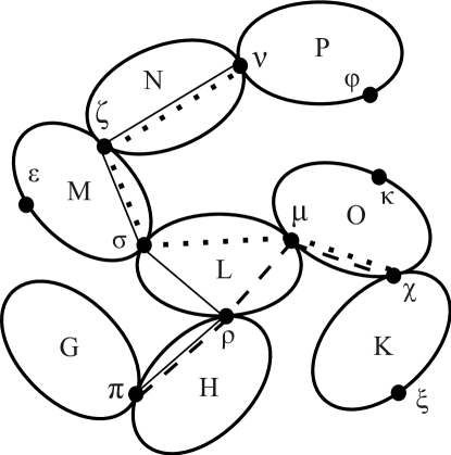
Figure 2: Diagrammatic representation the connectivity and vertices ($\nu$, $\rho$, $\zeta$, $\sigma$, $\mu$, $\chi$, $\pi$) and reference points ($\epsilon$, $\phi$, $\kappa$, $\xi$) of a star like structure composed of many sub-units. Shown on the figure are the path $P(\pi,\nu)$ connecting sub-unit $G$ and $P$ (solid), the path $P(\nu,\chi)$ connecting $P$ and $K$ (dotted), and the path $P(\pi,\chi)$ connecting $G$ and $K$ (dashed).

We can generate complex structures by joining sub-units at reference points to form vertices in the structure. Since a single sub-unit can have an arbitrary number of reference points associated with it, and we can join an arbitrary number of sub-units at a vertex, rather complex structures can be generated. A diagrammatic example of such a structure is shown in fig. 2, which shows a number of different sub-units (capital letters) connected by vertices (Greek letters). The structure has both one, two and three functional sub-units. Paths that connect specified vertices and reference points through such structures play a key role in the formalism we present below. On the figure is shown three examples of such paths connecting vertices. The structure also contains internal vertices joining sub-units and external “free” reference points. Further sub-units can be linked to the “free” reference points and to the internal vertices of the structure. Note that the same Greek vertex label is used in all the sub-units reference points linked to a vertex, such that we get branched structures where each vertex has a unique label. For a concrete example, polymer sub-units can be joined into a large variety of block-copolymer and branched structures by end-linking them. Alternatively, the sub-unit could be a block copolymer, a $f$-functional polymer star or a $g$’th generation dendrimer, and the more complex sub-units could be linked tip-to-tip to form chains.

The scattering from such a composite structure $S$ is defined analogously to the form factor of a single sub-unit as

$$F_{S}(q)\equiv\left(\sum_{I}\beta_{I}\right)^{-2}\left\langle\sum_{I,J}\sum_{i,j}b_{Ii}b_{Jj}e^{i{\bf q}\cdot({\bf r}_{Ii}-{\bf r}_{Jj})}\right\rangle_{S},$$ (4)

where the first sum is over sub-units. If we assume that joints are completely flexible such that sub-units joined by a common vertex can rotate freely with respect to each other, that the resulting branched structure does not contain any loops, and that all sub-units are mutually non-interacting, then we arrive at a scattering expression for the whole structure expressed exclusively in terms of the sub-unit scattering contributions (eqs. 1-3) as

$$=\beta_{S}^{-2}\left[\sum_{I}\beta_{I}^{2}F_{I}(q)+\sum_{\begin{subarray}{c}I\neq J\\ \alpha\in I\>\mbox{near}\>\omega\in J\end{subarray}}\beta_{I}\beta_{J}A_{I\alpha}(q)A_{J\omega}(q)\prod_{\begin{subarray}{c}(K,\tau,\eta)\\ \in\mbox{P}(\alpha,\omega)\end{subarray}}\Psi_{K\tau\eta}(q)\right].$$ (5)

Details of the derivation of this expression is given in the appendix. The total scattering length of the structure is $\beta_{S}=\sum_{I}\beta_{I}$. The structural form factor represents the site-to-site pair-correlation function of the structure build out of sub-units. It consists of two terms where the first is a sum over all contributions from all pairs of scatterers inside the same sub-unit, and the second term is double sum over all the interference contributions from pairs of scatterers residing in different sub-units. How should the sum in the second term be evaluated? For each distinct pair of sub-units $I$ and $J$ in the double sum, we identify the vertex $\alpha$ on sub-unit $I$ nearest to $J$ and vertex $\omega$ on sub-unit $J$ nearest to $I$. Here “near” means in terms of the shortest path originating at a vertex on $I$ and terminating at a vertex on $J$. We denote the path connecting $\alpha$ and $\omega$ through the structure $P(\alpha,\omega)$. For the product, we have to identify all sub-units $K$ on the path and also identify the vertices $\tau$ and $\eta$ across which the path traverses the sub-unit. This construction is always unique and well defined for structures that does not contain loops. While the expression for the structural form factor appears quite complex, this is mostly due to the notation we have had to introduce to describe general branched structures. In mathematical terms, structures such as the one shown in fig. 2 belong to the class of hypergraphs since not only can multiple sub-units share the same vertex, but a single sub-unit can also have multiple reference points.

The form factor expression (eq. 5) has a quite simple physical interpretation. The structural form factor is the pair-correlation function between all sites in the structure. This is obtained by propagating position information between all scattering sites in the structure. When both scattering sites belong to the same sub-unit this is given by the sub-unit form factors and is described by the first term. The distance information between scattering sites are on different sub-units is obtained by propagating position information along paths through the structure (using eq. 38 in the Appendix). To propagate site-to-site position information between scatterers in sub-unit $I$ and scatterers in sub-unit $J$, we first have to propagate the position information between the scattering sites in sub-unit $I$ to the vertex $\alpha$ nearest $J$. This is done by the form factor amplitude $\beta_{I}A_{I\alpha}$. The position information is then propagated along the path of intervening sub-units towards the vertex $\omega$ on sub-unit $J$, which is nearest $I$. Each time a sub-unit is traversed it contributes a phase factor $\Psi_{K\tau\eta}$ to account for the conformationally averaged distance between the two vertices. Finally the position information is propagated between the vertex $\omega$ and the scattering sites inside the $J$ sub-unit. This is done by the final form factor amplitude $\beta_{J}A_{J\omega}$. Only the amplitudes has a scattering length prefactor, since they represent the amplitudes of scattered waves from all the scatterers inside the sub-units relative to the $\alpha$ and $\omega$ vertices while the product of phase factors represent excess phase contributed by the path between the vertices. The product of all these propagators describe the scattering length weighted interference contribution from the $I$’th and $J$’th sub-units. The same process can be described in real space, where the product of propagators becomes a convolution of the site-to-vertex, vertex-to-vertex, and vertex-to-site sub-unit pair-correlation functions that the propagators represent. This convolution produces the excess scattering length weighted site-to-site pair-correlation function for sub-units $I$ and $J$. Since the pair-distances between $J$ and $I$ also contribute all interference terms are counted twice in the structural form factor.

In fig. 2, we show multiple connected sub-units to illustrate how to calculate some of the interference contributions in more detail, and how to find the closest vertices and paths through a branched structure. For neighbors such as the $G$ and $H$ sub-units, the vertex $\pi$ on $G$ is nearest $H$, just as it is the vertex on $H$ nearest $G$. Hence $\alpha=\omega=\pi$, and the path of sub-units between them $P(\alpha,\omega)=P(\pi,\pi)=\{\}$ is the empty set. The product over the empty set is unity by definition. The $G$ and $H$ sub-unit pair contributes a scattering term $\beta_{G}\beta_{H}A_{G\pi}A_{H\pi}$. For next nearest neighbors such as $M$ and $P$, the vertex $\zeta$ on $M$ is nearest $P$, while $\nu$ on $P$ is nearest $M$. The path between the two vertices traverses the $N$ sub-unit across the $\zeta$ and $\nu$ vertices: $P(\zeta,\nu)=\{(N,\zeta,\nu)\}$. The sub-unit pair $M$ and $P$ contributes an interference term $\beta_{M}\beta_{P}A_{M\zeta}\Psi_{N\zeta\nu}A_{P\nu}$. For second nearest neighbors such as $N$ and $O$, the path runs between $\zeta$ and $\mu$, and the path is $P(\zeta,\mu)=\{(M,\zeta,\sigma),(L,\sigma,\mu)\}$. Hence the sub-unit pair $N$ and $O$ contributes a term $\beta_{N}\beta_{O}A_{N\zeta}\Psi_{M\zeta\sigma}\Psi_{L\sigma\mu}A_{O\mu}$. Three long paths are shown in the figure. The sub-units $G$ and $P$ contribute a term $\beta_{G}\beta_{P}A_{G\pi}\Psi_{H\pi\rho}\Psi_{L\rho\sigma}\Psi_{M\sigma\zeta}\Psi_{N\zeta\nu}A_{P\nu}$, the sub-units $P$ and $K$ contribute a term $\beta_{K}\beta_{P}A_{K\chi}\Psi_{O\chi\mu}\Psi_{L\mu\sigma}\Psi_{M\sigma\zeta}\Psi_{N\zeta\nu}A_{P\nu}$, and the sub-units $G$ and $K$ contribute a term $\beta_{G}\beta_{K}A_{G\pi}\Psi_{H\pi\rho}\Psi_{L\rho\mu}\Psi_{O\mu\chi}A_{K\chi}$. The reference points $\epsilon$, $\varphi$, $\xi$ , and $\kappa$ can be used to add further sub-units to the structure, but the form factor is independent of these since no path between vertices will ever start at, terminate at, or traverse an exterior reference point.

Note that the assumptions of flexible joints, mutually non-interacting sub-units, and branched structures without loops allows us to exactly derive the form factor of the whole structure without making any assumptions about the specific structure inside the sub-units. In this sense, the scattering from factor is general as it allows us to write down scattering expressions for a connected structure without a priori knowledge of the sub-units that the structure is build of. If any of these assumptions are not strictly fulfilled, then the structural scattering expression above can be regarded as the zeroth order term in an perturbation expansion of these effects. Whether this is a good or bad approximation depends on the detailed structures in the sub-units and their interactions. A special case of this expression was derived and used for two functional polymer structures in refs. Benoit and Hadziioannou (1988); Read (1998); Pedersen (2002).

Using eq. 5, we can calculate the form factor for a whole structure in terms of the fundamental sub-units it is build of. However, when modeling the scattering from complex structures it is advantageous to be able selectively modify parts of the structure while retaining the rest, or to add more sub-units to an existing structure. To model the resulting change in the scattering spectrum, it is advantageous also to derive the form factor amplitudes and phase factors of the whole structure. The form factor amplitude of the whole structure relative to the reference point or vertex $\alpha$ is defined as

$$A_{S\alpha}(q)\equiv\left(\sum_{I}\beta_{I}\right)^{-1}\left\langle\sum_{I}\sum_{k}b_{Ik}e^{i{\bf q}\cdot({\bf r}_{Ik}-{\bf R}_{T\alpha})}\right\rangle_{S},$$ (6)

again with the same assumptions as for the form factor of the structure, we can rewrite express the form factor amplitude of the whole structure in terms of the sub-unit scattering contributions as

$$=\beta_{s}^{-1}\left[\sum_{\begin{subarray}{c}I\\ \omega\in I\,\mbox{near}\,\alpha\end{subarray}}\beta_{I}A_{I\omega}(q)\prod_{\begin{subarray}{c}(K,\tau,\eta)\\ \in\mbox{P}(\alpha,\omega)\end{subarray}}\Psi_{K\tau\eta}(q)\right].$$ (7)

Again, we refer to the Appendix for details. Here the sum denotes, that on each sub-unit $I$, we have to identify the vertex on the sub-unit $\omega$, that is nearest $\alpha$ in terms of structural connectivity. For each vertex a structure has, there will be a corresponding form factor amplitude. We can also define and derive the phase factor between any two vertices on the whole structure as

$$\Psi_{S\alpha\omega}(q)\equiv\left\langle e^{i{\bf q}\cdot({\bf R}_{T\alpha}-{\bf R}_{T\omega})}\right\rangle_{S}=\prod_{\begin{subarray}{c}(K,\tau,\eta)\\ \in\mbox{P}(\alpha,\omega)\end{subarray}}\Psi_{K\tau\eta}(q).$$ (8)

The structural form factor amplitude and phase factor also have simple physical interpretations despite their complex appearance. The structural form factor amplitude propagates position information between the vertex or reference point $\alpha$ and all scattering sites in the structure. For a particular sub-unit $I$ and vertex $\omega$ nearest $\alpha$, we first first have to propagate position information between $\alpha$ and the end $\omega$ vertex on the path path $P(\alpha,\omega)$. Each sub-unit the path traverses contributes a phase factor $\Psi_{K\rho\sigma}$. Then position information is propagated between the $\omega$ vertex and all the sites inside the $I$’th sub-unit, which is represented by the form factor amplitude $A_{I\omega}$. The product of all the propagators produces the form factor amplitude which represent the total amplitude of scattered waves from scattering sites in the structure measuring the phase relative to the $\alpha$ reference point or vertex. The same process can be described In real space, where the product of propagators becomes a convolution of the vertex/reference point-to-vertex and vertex-to-site sub-unit pair-correlation functions that the propagators represent. This convolution produces the excess scattering length weighted site-to-vertex/reference point pair-correlation function for the whole structure. The interpretation of the structural phase factor is that it propagates distance information between the vertex/reference point $\alpha$ and the vertex/reference point $\omega$. This is the product of all the phase factors $\Psi_{K\rho\sigma}$ for each sub-unit that has to be traversed on the path $P(\alpha,\omega)$ through the structure. The phase factor represent the phase difference between two reference points or vertices in the structure averaged over the conformation and orientations of all sub-units in the structure.

Having defined and derived the form factor amplitudes and phase factors of a general structure, we have completed the formalism in the sense that we can now regard any structure described by the formalism as a sub-unit in the formalism itself. This enables us to compose and combine several structures to build new structures. For instance, if a new structure $R$ is formed by joining two known structures $S$ and $T$ at a common vertex $\alpha$, then the form factor, form factor amplitude of the resulting structure can be derived from eqs. 5, 7. They are given by

$$F_{R}=\beta_{R}^{-2}\left(\beta_{S}^{2}F_{S}+\beta_{T}^{2}F_{T}+2\beta_{S}\beta_{T}A_{S\alpha}A_{T\alpha}\right),$$ (9)

$$A_{R\omega}=\beta_{R}^{-\text{1}}\left(\beta_{S}A_{S\omega}+\beta_{T}\Psi_{S\omega\alpha}A_{T\alpha}\right)\quad\mbox{if}\quad\omega\in S$$ (10)

where a similar expression applies for the form factor amplitude when $\omega\in T$ with $S$ and $T$ interchanged. Here the excess scattering length of the whole structure is $\beta_{R}=\beta_{S}+\beta_{T}$. The phase factors of the resulting structure $R$ are given by

$$\Psi_{R\rho\sigma}=\begin{cases}\Psi_{T\rho\alpha}\Psi_{S\alpha\sigma}&\quad\mbox{if}\quad\rho\in T,\sigma\in S\\ \Psi_{S\rho\alpha}\Psi_{T\alpha\sigma}&\quad\mbox{if}\quad\rho\in S,\sigma\in T\\ \Psi_{S\rho\sigma}&\quad\mbox{if}\quad\rho\in S,\sigma\in S\\ \Psi_{T\rho\sigma}&\quad\mbox{if}\quad\rho\in T,\sigma\in T\end{cases}.$$ (11)

These expressions also apply in the special case where one or both of the structures are single sub-unit, hence they allow us to grow the scattering expressions for a structure by progressively growing the structure one sub-unit or sub-structure at the time. Another operation is to delete a sub-unit $K$ from a given structure, the simplest way is to collapse all vertices to a single non-scattering point: this is done by the substitution $F_{K}=0$,$A_{K\cdot}=0$,$\beta_{K}=0$ and $\Psi_{K\cdot\cdot}=1$ where $\cdot$ denotes any vertex of the $K$’th sub-unit.

What have we learned by this exercise? We have expressed the three scattering expressions for a whole structure (eqs. 5, 7, and 8) in terms of three scattering expressions for the sub-units (eqs. 1, 2, 3) that the structure is composed of. The structural scattering expressions are generic in the sense that they has been formulated without making any assumptions of the internal structure of the sub-units. The price we pay for this is that the formalism is only exact for mutually non-interacting sub-units that are joined by completely flexible joints. The formalism makes it easy to derive the form factors of hierarchies of progressively more complex structures. We have, for instance, shown how to generate a new structure by two sub-units together and to delete sub-units. Repeating these operations allows us to join multiple structures together and remove parts of the structures again. We can also replace sub-units by sub-units with another structure, or even identify sub-unit motifs and replace them by other motifs when they have the same external vertices. The price we pay to be able to generate structures from structures is that none of these structures can contain loops. To summarize, the present formalism allows us to construct scattering expressions for a large class of structures, and we have formulated it in a way that allows us to easily write a computer program or use computer aided algebra programs to construct scattering expressions and evaluating them for any given structure.

The diagrammatic interpretation of the formalism establishes a direct mapping between the sub-units and the structural connectivity on the one hand and on the other hand the algebraic structure of the structural scattering expressions. If we generate a new structure by any of the structural transformations above, the diagrammatic interpretation allows us to directly write down the corresponding algebraic transformation of the scattering expressions. Having proved the validity of diagrammatic interpretation by deriving the structural scattering expressions, we can in essence forget these complicated equations and remember only their simple diagrammatic interpretation, as it allows to write down the general structural scattering expressions and apply them to any structure described by the formalism.

III Generic ABC structure

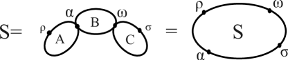
Figure 3: A structure $S$ composed of three sub-units $A$, $B$, and $C$ that are joined at two vertices $\alpha$ and $\omega$ and has two reference points $\rho$ and $\sigma$. (left) The whole structure can equally well be regarded as a single four functional sub-unit with an internal $ABC$ structure. (right)

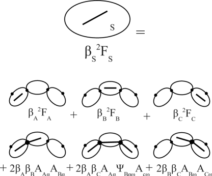
Figure 4: Form factor of the structure shown in fig. 3 along all the contributing terms and their diagrammatic representations.

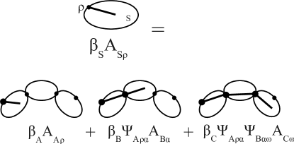
Figure 5: Form factor amplitude of the structure shown in fig. 3 relative to the $\rho$ vertex along with all the contributions and their diagrammatic representation.

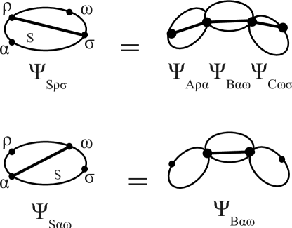
Figure 6: Phase factors the structure shown in fig. 3 between the $\rho$ and $\sigma$ vertices and beween the $\alpha$ and $\omega$ vertices.

In fig. 3, we shown the simple $ABC$ structure where three sub-units have been joined by two vertices to form a linear chain. This could for instance describe a tri-block copolymer if the three sub-units are polymers, but it could also describe two colloidal particles bridged by an adsorbed polymer, or a protein with two dangling tails. Since we have both eq. 5, 7, and 8 we can derive all the scattering terms describing the structure, and hence regard the whole structure as a single sub-unit $S$ characterized by four vertices/reference points. In Fig. 4 we show all the terms that contribute to the form factor, in fig. 5 we show all the terms that contribute to the form factor amplitude relative to $\rho$, and in fig. 6 we show two of the phase factors characterizing the $ABC$ structure. Similarly we could specify the form factor amplitudes relative to all other reference points or vertices and phase factors between all reference points or vertices. The diagrammatic representation illustrates how all possible pair-distances between the sub-units are accounted for by similar terms in the scattering expressions for the structure. In a similar way, we can directly write down the generic scattering expressions for any branched structure of sub-units that we can imagine.

IV Two functional sub-units

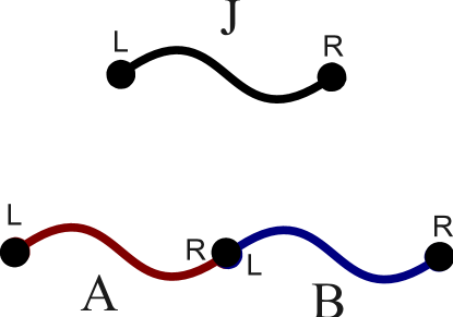
Figure 7: A linear sub-unit $J$ shown as a line connecting the left and right ends (denoted $L$ and $R$). Also shown is an $AB$ structure where the right end of $A$ is linked to the left end of $B$.

In the following, we will focus on how the general formalism can be applied to derive the scattering expressions for structures build of sub-units and structures with only two reference points. We refer to these as the “left” and “right” ends. This is illustrated in fig. 7. The sub-unit could for instance be polymers or rigid rods. These are symmetric in the sense that the scattering from a structure is unaffected if we flip the ends of a polymer or rod sub-unit (assuming a constant scattering length density along the sub-unit). The sub-units could also be more complex asymmetric structures such as $AB$ block copolymers, where the scattering from a structure will change if we flip a $AB$ block-copolymer turning it into a $BA$ block-copolymer (e.g. $ABC$ and $BAC$ structures will produce different scattering spectra). We can also regard any complex branched structure as being effectively two functional, if we choose two special vertices or reference points in the structure and regard these as the “left” and “right” ends of the structure. For instance for a star, we can pick the tips of two arms as the reference points.

For two functional sub-units, the $J$’th sub-unit is completely characterized by $F_{J}$, $A_{JR}$, $A_{JL}$, and $\Psi_{J}$ which denote the form factor, form factor amplitude relative to the left/right ends and phase factor between the left and right ends of the sub-unit, respectively. In the following, instead of using Greek indices for reference points/vertices we will instead use “left” and “right” ends denoted by subscripts $L$ and $R$ as illustrated in fig. 7. The scattering from an $AB$ structure where the right end of $A$ is joined with the left end of $B$ is a special case of eqs. (9-11). The scattering from an $AB$ structure is given by

$$F_{AB}(q)=\left(\beta_{A}+\beta_{B}\right)^{-2}\left[\beta_{A}^{2}F_{A}+\beta_{B}^{2}F_{B}+2\beta_{A}\beta_{B}A_{AR}A_{BL}\right],$$ (12)

$$A_{AB,L}(q)=\left(\beta_{A}+\beta_{B}\right)^{-1}\left[\beta_{A}A_{AL}+\beta_{B}\Psi_{A}A_{BL}\right],$$ (13)

$$A_{AB,R}(q)=\left(\beta_{A}+\beta_{B}\right)^{-1}\left[\beta_{B}A_{BR}+\beta_{A}\Psi_{B}A_{AR}\right],$$ (14)

$$\Psi_{AB}(q)=\Psi_{A}\Psi_{B}.$$ (15)

Here we choose the free end of the $A$ sub-unit as the “left” end, while the free end of the $B$ sub-unit is the “right” end. We can also easily simplify the scattering expressions from the $ABC$ structure to produce an effective two functional structure analogously to the $AB$ structure.

V Polymer special case

In the present paper, we focus on scattering expressions of complex structures. The functions that represent the internal structure of various sub-units are presented in an accompanying paper.cs_ . However, here we will (re)derive the functions representing a flexible polymer. Polymers deserves special attention, since they are the most important building block of a large variety of synthetic branched molecular structures. A di-block copolymer $AB$ Leibler (1980); Leibler and Benoit (1981) consists of two polymer molecules $A$ and $B$ linked end-to-end. The polymers are symmetric, hence the left and right form factor amplitudes for the sub-units are identical, and we can discard the $L$ and $R$ subscripts in eqs. (12-15).

Single polymer with $n$ monomers can equally well be regarded as a di-block copolymer of two identical blocks of $n/2$ monomers each ($\beta_{A}=\beta_{B})$. The form factor, form factor amplitude, and phase factor are dimensionless numbers. Hence they depend not only on $q$, which has units of reciprocal length, but also a characteristic length scale of the polymer. Choosing the radius of gyration $R_{g}^{2}=b^{2}n/6$ where $b$ is the step length and $n$ the number of steps, we can define a dimensionless parameter $x=q^{2}R_{g}^{2}$. The $n$-monomer long AB polymer is characterized by the three functions $F_{AB}=F_{polymer}(x)$, $A_{AB}=A_{polymer}(x)$, and $\Psi_{AB}=\Psi_{polymer}(x)$ while the two $n/2$-monomer long $A$ and $B$ polymers are characterized by $F_{A}=F_{B}=F_{polymer}(x/2)$, $A_{A}=A_{B}=A_{polymer}(x/2$), and $\Psi_{A}=\Psi_{B}=\Psi_{polymer}(x/2)$. Requiring the scattering from the $AB$ polymer is identical to that of the $A$ and $B$ end-linked polymers of half the number of monomers in eqs. (12-15) produce the following functional equations

$$F_{polymer}(x)=\frac{1}{2}\left[F_{polymer}\left(\frac{x}{2}\right)+A_{polymer}^{2}\left(\frac{x}{2}\right)\right],$$ (16)

$$A_{polymer}(x)=\frac{1}{2}A_{polymer}\left(\frac{x}{2}\right)\left[1+\Psi_{polymer}\left(\frac{x}{2}\right)\right],$$ (17)

and

$$\Psi_{polymer}(x)=\Psi_{polymer}^{2}\left(\frac{x}{2}\right).$$ (18)

The latter equation has the obvious solution $\Psi_{polymer}(x)=\exp(-\alpha x)$. Here $\alpha$ is a scaling factor that we set to unity without loss of generality, since it corresponds to a trivial rescaling of $x$. Using the ansatz $A_{polymer}(x)=1+\sum_{n=1}^{\infty}\alpha_{n}x^{n}$ and Taylor expanding both sides of eq. (17) and applying the same approach to the form factor we obtain the polymer solutions

$$\Psi_{polymer}(x)=\exp(-x),\quad A_{polymer}(x)=\frac{1-\exp(-x)}{x},$$ (19)

$$\mbox{and\quad}F_{polymer}(x)=\frac{2[\exp(-x)-1+x]}{x^{2}}.$$ (20)

These results we previously obtained by HammoudaHammouda (1992) and DebyeDebye (1947) by performing the conformational and orientational averages of eqs. (1-3) explicitly for the Gaussian pair-distance distributions characterizing a random walk. Here these solutions emerge as a self-consistency check of the present formalism, when requiring self-similarity of an object with fractal dimension two when undergoing a particular scaling transformation. Note that we could not have obtained the form factor expression unless we had all three structural scattering expressions.

A polymer sub-unit is completely characterized by the triplet of form factor, form factor amplitudes and phase factors. The scattering expression for an flexible ABC block-copolymer is obtained by setting $F_{A}(q)=F_{polymer}(R_{gA}q)$, $A_{A}(q)=A_{polymer}(R_{gA}q)$, and $\Psi_{A}(q)=\Psi_{polymer}(R_{gA}q)$ and similar for the B and C blocks in the generic ABC structure, where $R_{gA}$, $R_{gB}$, $R_{gC}$ denotes the radii of gyration of the three blocks in figs. 4-5. This is a concrete example of how the present formalism allows us to write down generic structural scattering expressions and choose which triplets should be used to characterize the internal structure of the sub-units. Note that these scattering expressions are specific to polymers, all other scattering expressions in this paper are generic in the sense that they remain valid irregardless of what sub-unit structures are chosen.

VI Chain structures

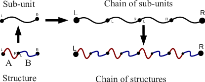
Figure 8: Building a chain of $N$ left-end to right-end linked sub-units. Substituting the chain sub-unit with any sub-structure produces a chain of such structures, here is shown the result of substituting an $AB$ structure to produce a chain of alternating sub-units.

Fig. 8 shows how a linear chain can be build by $N$ repeated sub-units joined left end to right end. We regard the chain as an effective two functional structure defined by the left and right free ends. In the case of a chain, the scattering expressions (eqs. 5-8) becomes

$$F_{chain}(q)=\frac{F}{N}+\frac{2A_{R}A_{L}}{N^{2}}\left((N-1)+(N-2)\Psi+(N-3)\Psi^{2}+\cdots+2\Psi^{N-3}+\Psi^{N-2}\right)$$ (21)

$$=\frac{F}{N}+2\frac{\Psi^{N}-N\Psi+N-1}{N^{2}(\Psi-1)^{2}}A_{R}A_{L}.$$ (22)

The terms of the form $2C_{n}A_{L}\Psi^{n}A_{R}$ encode the fraction of neighbors pairs $n$ sub-units distant from each other. The form factor amplitude of a chain relative to the left end is given by

$$A_{chain,L}(q)=\frac{A_{L}}{N}(1+\Psi+\Psi^{2}+\cdots+\Psi^{N-1})=\frac{A_{L}}{N}\frac{\Psi^{N}-1}{\Psi-1}.$$ (23)

Here the prefactors of the $B_{n}A_{L}\Psi^{n}$ encode the fraction of units that are a certain distance from the vertex $\alpha$. A identical expression exists for the right end (denoted $R)$ with $L$ replaced by $R$. Finally the phase factor between the two ends becomes

$$\Psi_{chain}(q)=\Psi^{N}.$$ (24)

VII Substitution

Except for the polymer, all the expressions presented above are generic in the sense that they have been derived without making any assumptions about the internal structure of the sub-units themselves. If we, for instance, insert the polymer scattering expressions into these generic expressions the result become the specific scattering expressions for di- and tri-block copolymers and end-linked chains of polymers. Since we also have derived not only the form factor, but also the form factor amplitudes and phase factors for these generic structures, we have completed the formalism, such that we can also use a whole structure as a sub-unit to build more complex generic structures. For example, a $ABAB\cdots AB$ structure is a chain of $N$ repeated $AB$ structures as shown in fig. 8. We can generate the corresponding generic structural scattering expressions by combining the $N$-repeated chain expressions (eqs. 22-24) with those of an $AB$ structure (eqs. 12-15). This is done by the substitution $F\rightarrow F_{AB}$, $A_{R}\rightarrow A_{AB,R}$, $A_{L}\rightarrow A_{AB,L}$, $\Psi\rightarrow\Psi{}_{AB}$ in eq. 22. The result for the generic $AB$ $N$-repeated chain form factor is trivially obtained as

$$F_{chain,AB}(q)=\frac{1}{N\left(\beta_{A}+\beta_{B}\right)^{2}}\left[\beta_{A}^{2}F_{A}+\beta_{B}^{2}F_{B}+2\beta_{A}\beta_{B}A_{AR}A_{BL}\right]$$

$$+2\frac{\Psi_{A}^{N}\Psi_{B}^{N}-N\Psi_{A}\Psi_{B}+N-1}{N^{2}\left(\Psi_{A}\Psi_{B}-1\right)\left(\beta_{A}+\beta_{B}\right)^{2}}\left[\beta_{A}A_{AL}+\beta_{B}\Psi_{A}A_{BL}\right]\left[\beta_{B}A_{BR}+\beta_{A}\Psi_{B}A_{AR}\right],$$ (25)

in a similar way, we can easily obtain the left and right form factor amplitudes and the phase factor for this structure. If we had substituted $F_{A}\rightarrow F_{chainA}$, $A_{AR}\rightarrow A_{chainA,R}$, $A_{AL}\rightarrow A_{chainA,L}$, $\Psi_{A}\rightarrow\Psi{}_{chainA}$ and similar for sub-unit $B$ in eq. 12, then the result would have been the generic form factor for an $AA\cdots AABB\cdots BB$ structure. Inserting the polymer expressions (eqs. 19-20) in these generic expressions would specialize them to produce the corresponding block-copolymer scattering expressions. We could, for instance, also choose other sub-units e.g. rods and insert the corresponding scattering expressions for a rod sub-unit to specialize the generic scattering expression above for a chain of alternating polymers and rods. Since we can also easily calculate the form factor amplitudes and phase factor for these structures, these expressions can also serve as sub-units to build more complex structures out of alternating chains of sub-units.

VIII Star structures

The simplest branched structure is that of a star. The scattering from a polymeric star was derived by Benoit.Benoit (1953); Berry and Orofino (1964); Burchard (1974) The generic scattering expression for a star structure of $f$ identical sub-unit arms attached by their left end to a central point follows from 5 as

$$F_{star}(q)=\frac{1}{f}\left[F+(f-1)A_{L}^{2}\right].$$ (26)

The star has $fF$ contributions from the form factor of each arm, while there are $f(f-1)A_{L}^{2}$ interference contributions between the arms, since the first scatterer can be on any of the $f$ arms, while the second scatterer can be one of the remaining $f-1$ arms. We normalize with the total number of contributions which is $f^{2}.$ Each interference term contributes $A_{L}^{2}$ since the two arms are joined by their left end. Since all arms are joined by the common center of the star there are no phase factors.

To make the star an effectively two-functional sub-unit, we can pick two vertices as the “left” and “right” ends to express the star form factor amplitude and phase factors. There are two natural options: The free end of an arm (denoted “e”) or the center of the star (denoted “c”), which leads to three possible structures center-to-center (“cc”), center-to-end (“ce”), or end-to-end (“ee”). Their form factor amplitudes and phase factors are given by

$$A_{star,e}(q)=\frac{1}{f}\left[A_{R}+(f-1)\Psi A_{L}\right],\quad\mbox{{and}\quad}A_{star,c}(q)=A_{L}.$$ (27)

$$\Psi_{star,cc}(q)=1,\quad\Psi_{star,ce}(q)=\Psi,\quad\mbox{{and}\quad}\Psi_{star,ee}(q)=\Psi^{2}.$$ (28)

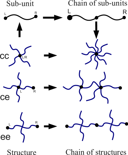
Figure 9: Comparison between the chain structures produced when substituting the sub-unit for a center-to-center, center-to-end and end-to-end star.

Fig. 9 shows the effect of the three substitutions

$$F\rightarrow F_{star}\quad\quad A_{L}\rightarrow A_{star,c}\quad\quad A_{R}\rightarrow A_{star,c}\quad\quad\Psi\rightarrow\Psi_{star,cc},$$

$$F\rightarrow F_{star}\quad\quad A_{L}\rightarrow A_{star,c}\quad\quad A_{R}\rightarrow A_{star,e}\quad\quad\Psi\rightarrow\Psi_{star,ce},$$

and

$$F\rightarrow F_{star}\quad\quad A_{L}\rightarrow A_{star,e}\quad\quad A_{R}\rightarrow A_{star,e}\quad\quad\Psi\rightarrow\Psi_{star,ee},$$

in a chain of $N=2$ repeating sub-units. The result is respectively a center-to-center, center-to-end and end-to-end linked stars. The center-to-center linking produces a $Nf$ functional star, while the center-to-end linking produces a bottle brush with a $f-1$ functional end and $f+1$ functional branching points inside the bottle brush and a single arm joining each branch point. End-to-end linking produces a bottle brush with $f$ functional branch points and where the branch points are separated by two arms lengths. These structures are geometrically restricted in the sense that the star centers are separated by zero, one or two arms lengths. We can obtain more control over the bottle-brush structure by having a flexible spacer sub-unit between the stars. Using the $ABAB\cdots AB$ structure with $A$ being a center-to-center $f$-functional star, and $B$ a spacer sub-unit produces the form factor of a bottle brush, this is obtained by the following substitutions in eq. 25

$$F_{A}\rightarrow F_{star}\quad\quad A_{AL}\rightarrow A_{star,c}\quad\quad A_{AR}\rightarrow A_{star,c}\quad\quad\Psi_{A}\rightarrow\Psi_{star,cc},$$

and

$$F_{B}\rightarrow F_{s}\quad\quad A_{BL}\rightarrow A_{s,L}\quad\quad A_{BR}\rightarrow A_{s,R}\quad\quad\Psi_{B}\rightarrow\Psi_{s}.$$

Here $F_{s}$, $A_{s,L}$, $A_{s,R}$, $\Psi_{s}$ characterizes the spacer, which could e.g. be given by the polymer expressions eqs. 19-20. Since these expressions are obtained by trivial substitutions, we shall not state them here for sake of brevity. The scattering from a bottle brush with random positions of the polymeric side-chains was derived by Casassa and BerryCasassa and Berry (1966); Pedersen (1997). The generic scattering expressions for a miktoarm star structure with two types of arms can be produced from the $AB$ structure, where each sub-unit is substituted for stars that are linked center-to-center. Similarly we can obtain the generic scattering expressions for a pom-pom structure by specializing the $ABC$ structure (fig. 4) to represent two identical center-to-center stars ($A$ and $C$) separated by a spacer ($B$) sub-unit:

$$F_{pompom}(q)=\left(2\beta_{star}+\beta_{s}\right)^{-2}\left[2\beta_{star}^{2}F_{star}+\beta_{s}^{2}F_{s}\right.$$

$$\left.+2\beta_{star}\beta_{s}A_{star,c}(A_{s\text{L}}+A_{sR})+2\beta_{star}^{2}A_{star,c}^{2}\Psi_{s}\right]$$ (29)

inserting the expressions for the stars eqs. (26-28), and using the polymer expressions eqs. (19-20) for all sub-units produces the scattering expressions for a pom-pom polymer. If we want the scattering expression for a pom-pom where the arms are made of block-copolymers, we use the $ABAB\cdots AB$ structure eq. 25 and the corresponding form factor amplitudes and phase factor for the arms in the star expressions, and afterwards insert the polymer expressions for the $A$ and $B$ block copolymers. We could also use a rigid rod for the spacer, or for all sub-units to produce the scattering expressions for pom-poms build with rods.cs_ We shall not state the scattering expressions for any of these specific structures as these any many others can be obtained by trivial algebraic substitutions of the generic scattering expressions already given above.

IX Dendrimer structures

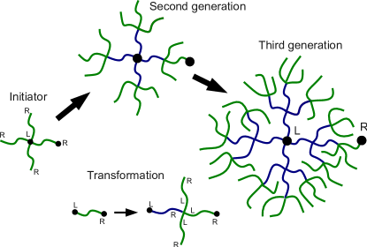
Figure 10: Generating the $g+1$’th generation Cayley tree by substituting each leaf (green) in the $g$’th generation Cayley tree (or an initiator $g=1)$ by a star with one dead branch (blue) and $f-1$ live leaves (green). Notice how the sub-unit ends are attached in the Initiator and the Transformation rule. On Initiator, the second, and third generation dendrimers we also show the two vertices we have chosen for “left” and “right” ends to make the dendrimer an effective two functional sub-unit.

One dendrimer structure is of particular interest, namely the Cayley tree. The Cayley tree has a regular structure, where all the branching points has the same functionality. A Cayley tree structure can be generated by repeated application of a transformation rule: Starting from an initiating $f$-functional star, each arm in the initiator star (or leaf in the dendrimer) is replaced by a $f$ functional star, where one arm is a “dead” branch connecting to the rest of the dendrimer and the remaining $f-1$ “live” leaves can grow further. This is illustrated in fig. 10.

The scattering functions for a Cayley tree can be generated by performing by performing the algebraic equivalent of the structural transformation on the initiator: Starting from the scattering expressions for the initiator, and replacing the terms characterizing each arm (or leaf) for the scattering expressions of a $f$ functional star, where each leaf is converted into a “dead” branch connected to $f-1$ leaf expressions can be substituted further to generate the next generation. By starting with an initiator star where all arms are linked to the center by their left end, and replacing each leaf by a star where the right end of the dead branch is joined to the left end of the live leaves we can generate a dendrimer where the left end of all sub-units connects to the center, and the right end connects to the periphery of the dendrimer.

The initiator ($I$) is characterized by the following scattering expressions

$$F_{I}(q)=f^{-1}\beta_{1}^{2}\left(F_{1}+(f-1)A_{1L}^{2}\right),\quad\quad A_{IL}(q)=\beta_{1}A_{1L},$$ (30)

$$A_{IR}(q)=\beta_{1}(A_{1R}+(f-1)\Psi_{1}A_{1L}),\quad\quad\Psi_{I}(q)=\Psi_{1}$$ (31)

here $f$ is the functionality of the initiator and $F_{1}$, $A_{1L}$, $A_{1R}$, $\Psi_{1}$ characterizes the sub-units of the first generation. The arms in the star are joined by their left ends. For sake of algebraic simplicity we do not try to keep the expressions normalized. The unnormalized scattering expressions for the $2$nd generation dendrimer can be generated by performing the substitutions below with $g=1$ in the initiator expression, and in general the $g+1$’th generation dendrimer scattering expression can be generated by applying the substitutions below in with in the $g$’th generation of the scattering expressions:

$$F_{g}\rightarrow\beta_{g}^{-2}\left(\beta_{g}^{2}F_{g}+(f-1)\beta_{g+1}^{2}F_{g+1}\right.$$

$$\left.+2(f-1)\beta_{g}\beta_{g+1}A_{g,R}A_{g+1,L}+2(f-1)(f-2)\beta_{g+1}^{2}A_{g+1,L}^{2}\right)$$ (32)

$$A_{g,L}\rightarrow\beta_{g}^{-1}\left(\beta_{g}A_{g,L}+(f-1)\beta_{g+1}\Psi_{g}A_{g+1,L}\right)$$ (33)

$$A_{g,R}\rightarrow\beta_{g}^{-1}\left(\beta_{g}\Psi_{g+1}A_{g,R}+\beta_{g+1}\left[A_{g+1,R}+(f-2)\Psi_{g+1}A_{g+1,L}\right]\right)$$ (34)

$$\Psi_{g}\rightarrow\Psi_{g+1}\Psi_{g}$$ (35)

These rules are the algebraic equivalents of the structural transformation where each “live” $g$-generation leaf is converted into a dead $g$-generation branch ($g$ terms on the right hand side of the substitution), and $f-1$ live $g+1$-generation leaves (the $g+1$ terms). The new leaves are characterized by $F_{g+1}$, $A_{g+1,L}$, $A_{g+1,R}$, $\Psi_{g+1}$ which allows different sub-units to be used in the various generations of branches and leafs in the dendrimer. After iterated substitutions starting from the initiator scattering expressions we obtain the generic scattering expressions for any generation Cayley tree. Inserting the polymer expressions (eqs. 19-20) into the expressions will specialize them to a polymeric dendrimer.Burchard et al. (1984); Hammouda (1992); Boris and Rubinstein (1996) Alternatively, the $AB$ or $ABAB\cdots AB$ structure (eqs. 12-15 or 25) could be inserted to specialize the dendrimer scattering expression to provide the scattering expression of a dendrimers build out of diblock copolymers or copolymers with alternating blocks.

As for the stars, we have also chosen two vertices or reference points to turn the dendrimer into an effective two functional structure as shown in fig. 10. The “left” end is the center of the dendrimer, while the “right” end is the tip of a leaf. This allows us to use the dendrimer as a sub-unit, and inserting the generic dendrimer expressions into the chain will produce the generic scattering expression for a center-to-end or end-to-end linked chain of dendrimers.

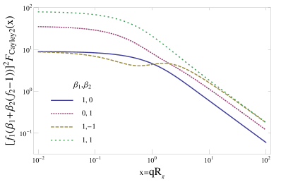
Figure 11: Unnormalized form factor of a second generation Cayley tree with $f=3$ for various choices of contrasts.

The effects of varying the contrast for a $3,3$ Cayley tree build out of identical polymer sub-units is shown in fig. 11. When the solvent matches the outer arms ($\beta_{2}=0$) only the scattering from the $3$ arms of the central star is shown, while only the scattering from the $6$ outer arms are shown when the solvent matches the inner star ($\beta_{1}=0$). At large $x$ this causes a factor $2$ upwards shift, while at small values of $x$ there are also interference contributions mediated by the central star. Comparing $\beta_{1}=\beta_{2}=1$ and $\beta_{1}=1=-\beta_{2}$ we observe the same scattering at large values of $x$ where the form factors of the sub-units dominate, but in the latter case the scattering at $x<1$ is reduced by almost an order of magnitude, since the interference contributions now reduce the scattering.

X Conclusions

A formalism for calculating the scattering branched structures composed of arbitrary sub-units of any functionality has been derived and presented. The formalism allows the scattering from a large class of complex heterogeneous structures to be derived with great ease. The formalism is exact in the case where all sub-units are mutually non-interacting, all sub-unit joins are completely flexible, and the branched structure does not contain any loops. We have also presented a diagrammatic illustration of the physical interpretation of the formalism, that allows us to draw a structure and write down the corresponding scattering expressions directly. The general formalism was simplified to the case of two-functional asymmetric sub-units, and illustrated by deriving generic scattering expressions for AB, ABC, chain structures, alternating chain structures as well as branched structures such as stars, pom-poms, bottle-brushes and dendrimers build out of unspecified sub-units.

A self-consistency requirement was used to derive the scattering expressions characterizing a polymeric sub-unit, however, none of the structural scattering expressions derived in the paper makes the assumption that the structures are build out of polymers. In fact, the scattering expressions are generic, in the sense that they remain valid irregardless of the internal structure the sub-units in the structure. In this sense, the formalism decompose scattering contributions due to the structural connectivity and due to the sub-unit internal structure.

The scattering contribution due to a sub-unit is completely described by a triplet of functions: phase factors, form factor amplitudes, and a form factor. The present formalism provides the triplet of scattering expressions for a whole structure build out of sub-units. The structural scattering expressions are complete in the sense that they allow a composite structure of multiple sub-units to be used as a single sub-unit within the formalism, which practically means inserting the three structural scattering expressions recursively into themselves. Complex hierarchical structures can be build by joining simple sub-units or complex sub-structures together one by one or by replacing all sub-units of a certain type by a more complex sub-structure.

A Feynman-like diagrammatic interpretation of the formalism allows us to map structural transformations to algebraic transformations of the scattering expressions. In this way, the present formalism allows us to build complex scattering expressions by simple algebraic transformations by inserting generic equations representing different structures into each other, or substituting specific sub-unit triplets for the three master equations of a sub-structure. We have illustrated this by deriving the algebraic transformation rules that will produce the form factor of dendrimer structures.

In an accompanying publication, we will review the sub-unit triplets of rigid rods, flexible and semi-flexible polymers, polymer loops, excluded volume polymers. We will also present triplets for thin disks and spheres, solid spheres and cylinders. We can regard these as infinity-functional sub-units when joining other sub-units to a random point on their surfaces. Finally, we will use the formalism presented here to predict the scattering from structures composed of mixtures of these sub-units.cs_ We hope that the formalism in the present paper will facilitate the analysis of experimental scattering data by allowing the scattering functions to be derived with greater ease for a large variety of complex structures.

XI Acknowledgments

C.S. gratefully acknowledges financial support from the Danish Natural Sciences Research Council through a Steno Research Assistant Professor fellowship. C.S. and J.S.P. gratefully acknowledges discussions with C.L.P. Oliveira.

Appendix

Assume that the $I$’th sub-unit is composed of point-like scatterers, where the $j$’th scatterer in the sub-unit is located at a position ${\bf r}_{Ij}$ and has excess scattering length $b_{Ij}$. Let ${\bf R}_{I\alpha}$ denote the position of the $\alpha$’th reference point associated with the $I$’th sub-unit. A reference point is a potential point for connecting the sub-unit to other sub-units. A single sub-unit can have an arbitrary number of such reference points associated with it. Once two or more sub-units are connected at the same reference point, we refer to it as a vertex in the resulting structure. Here and in the following capital letters refers to sub-units, lower case letters refers to scatterers inside a sub-unit, and Greek letters refers to vertices and reference points.

The structural form factor is defined in analogy with the sub-unit form factor (eq. 1) as

$$F_{S}(q)\equiv\left(\sum_{I}\beta_{I}\right)^{-2}\left\langle\sum_{I,J}\sum_{i,j}b_{Ii}b_{Jj}e^{i{\bf q}\cdot({\bf r}_{Ii}-{\bf r}_{Jj})}\right\rangle_{S}.$$ (36)

We can split the double sum into all the diagonal terms with $I=J$ and off diagonal terms with $I\neq J$ and interchange the order of the conformational averages and sums to produce

$$=\left(\sum_{I}\beta_{I}\right)^{-2}\left(\sum_{I}\left\langle\sum_{i,j}b_{Ii}b_{Ij}e^{i{\bf q}\cdot({\bf r}_{Ii}-{\bf r}_{Ij})}\right\rangle_{S}+\sum_{I\neq J}\left\langle\sum_{i,j}b_{Ii}b_{Jj}e^{i{\bf q}\cdot({\bf r}_{Ii}-{\bf r}_{Jj})}\right\rangle_{S}\right)$$ (37)

If we assume 1) that all sub-units are mutually non-interacting such that e.g. no excluded volume correlations exists between neighboring sub-units, 2) that all sub-unit pairs are joined by flexible links, such that no orientational correlations are be induced by the joints, and 3) that no loops exists in the structure such that the loop closure constraints introduces correlations between internal conformations, then the structural averages can be factorized into products of single sub-unit averages. Hence we can replace $\sum_{I}\langle\cdots\rangle_{S}$ by $\sum_{I}\langle\cdots\rangle_{I}$ in the first term, which by eq. 1 becomes the sum of the sub-unit form factors: $\sum_{I}\beta_{I}^{2}F_{I}(q)$.

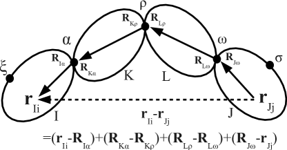
Figure 12: Vector between a pair of scattering sites ${\bf r}_{Ii}$ and ${\bf r}_{Jj}$ expressed in terms of steps traversing the intervening sub-units $K$ and $L$ and vertices $\alpha$, $\rho$, $\omega$ between the sub-units $I$ and $J$. Note the reference points of different sub-units are at identical locations in space because they are joined: ${\bf R}_{I\alpha}={\bf R}_{K\alpha}$, ${\bf R}_{K\rho}={\bf R}_{L\rho}$, and ${\bf R}_{L\omega}={\bf R}_{J\omega}$.

In the second term, we have weighted pair-distances between sites in the $I$ and $J$ sub-units. As shown in fig. 12, we can always project the vector ${\bf r}_{Ii}$-${\bf r}_{Jj}$ from the $i$’th scattering site on sub-unit $J$ to the $j$’th scattering site on sub-unit $I$ onto a path traversing through the structure. In the structure in fig. 12, we first a step from the $j$’th scattering site to the $\omega$ reference point on sub-unit $J$, a step through sub-unit $L$ from $\omega$ to $\rho$, a step through sub-unit $K$ from $\rho$ to $\alpha$, and finally from the $\alpha$ reference point to the $i$’th scattering site. Since we have assumed the structure does not contain loops the paths are always uniquely defined. In general, we have to find the reference point on sub-unit $I$ which is nearest to $J$ ($\alpha$ in fig. 12), and the reference point on sub-unit $J$ which nearest sub-unit $I$ ($\omega$ in fig. 12). Let $P(\alpha,\omega)$ denote the path of sub-units and vertices that has to be traversed between the two ends ($P(\alpha,\omega)=$$\{(K,\alpha,\rho),(L,\rho,\omega)\}$ in fig. 12). With these definitions, the general result for the distance is identity

$${\bf r}_{Ii}-{\bf r}_{Jj}=\left({\bf r}_{Ii}-{\bf R}_{I\alpha}\right)+\sum_{\begin{subarray}{c}(K,\tau,\eta)\\ \in\mbox{P}(\alpha,\omega)\end{subarray}}\left({\bf R}_{K\tau}-{\bf R}_{K\eta}\right)+\left({\bf R}_{J\omega}-{\bf r}_{Jj}\right)\quad\mbox{with\quad}\alpha\in I\>\mbox{near}\>\omega\in J.$$ (38)

Inserting this identity into the second term of eq. 37, and making use of the factorization of the conformational average into sub-unit averages yields

$$\left\langle\sum_{i,j}b_{Ii}b_{Jj}e^{i{\bf q}\cdot({\bf r}_{Ii}-{\bf r}_{Jj})}\right\rangle_{S}=\left\langle\sum_{i}b_{Ii}e^{i{\bf q}\cdot\left({\bf r}_{Ii}-{\bf R}_{I\alpha}\right)}\right\rangle_{I}\left\langle\sum_{j}b_{Jj}e^{i{\bf q}\cdot\left({\bf R}_{J\omega}-{\bf r}_{Jj}\right)}\right\rangle_{J}\prod_{\begin{subarray}{c}(K,\tau,\eta)\\ \in\mbox{P}(\alpha,\omega)\end{subarray}}\left\langle e^{i{\bf q}\cdot\left({\bf R}_{K\tau}-{\bf R}_{K\eta}\right)}\right\rangle_{K}$$ (39)

which by definition eqs. 2-3 become

$$=\beta_{I}A_{I\alpha}\beta_{J}A_{J\omega}\prod_{\begin{subarray}{c}(K,\tau,\eta)\\ \in\mbox{P}(\alpha,\omega)\end{subarray}}\Psi_{K\tau\eta}\quad\mbox{with\quad}\alpha\in I\>\mbox{near}\>\omega\in J.$$ (40)

This is the sub-unit interference scattering contribution which when inserted in eq. 37 becomes eq. 5. To obtain the form factor amplitude and phase factor of the whole structure (eqs. 7 and 8) exactly the same approach was applied using the following identities for the vector from a scattering site to a vertex or reference point and between two vertices or reference points

$${\bf r}_{Ii}-{\bf R}_{\alpha}=\left({\bf r}_{Ii}-{\bf R}_{I\omega}\right)+\sum_{\begin{subarray}{c}(K,\tau,\eta)\\ \in\mbox{P}(\alpha,\omega)\end{subarray}}\left({\bf R}_{K\tau}-{\bf R}_{K\eta}\right)\quad\mbox{with\quad}\omega\in J\>\mbox{near}\>\alpha,$$ (41)

and

$${\bf R}_{\alpha}-{\bf R}_{\omega}=\sum_{\begin{subarray}{c}(K,\tau,\eta)\\ \in\mbox{P}(\alpha,\omega)\end{subarray}}\left({\bf R}_{K\tau}-{\bf R}_{K\eta}\right).$$ (42)

Real-space

The form factor amplitude is the Fourier transform of the excess scattering length density distribution around a reference point. Hence we can directly obtain the (excess scattering length weighted) radial density distribution of the structure by an inverse Fourier transform asPedersen (2001)

$$\Delta\rho_{S\alpha}(r)=\int_{0}^{\infty}\mbox{d}q\frac{q\sin qr}{2\pi^{2}r}A_{S\alpha}(q).$$

We can also relate the structural scattering equations to mean-square distances of the structure. The radius of gyration has the general definition: $R_{g}^{2}=-\frac{3}{2}\left.\frac{d^{2}F(q)}{dq^{2}}\right|_{q=0}$. We can apply a Guinier expansionGuinier (1939) to each sub-unit as follows

$$F_{I}(q)=1-\frac{\langle R_{Ig}^{2}\rangle q^{2}}{3}+\cdots\quad A_{I\alpha}(q)=1-\frac{\langle R_{I\alpha}^{2}\rangle q^{2}}{6}+\cdots\quad\Psi_{I\sigma\rho}(q)=1-\frac{\langle R_{I\rho\sigma}^{2}\rangle q^{2}}{6}+\cdots.$$ (43)

Here $\langle R_{Ig}^{2}\rangle$, $\langle R_{I\alpha}^{2}\rangle$, and $\langle R_{I\rho\sigma}^{2}\rangle$ denote the radius of gyration, mean-square distance between all scattering sites and the vertex $\alpha$, and the mean-square distance between the vertices $\rho$ and $\sigma$ on the $I$’th sub-unit, respectively. The radius of gyration measures the mean-square distance between unique pairs of sites, hence there is a factor of two to avoid double counting. The general equation for the apparent radius of gyration can be obtained by differentiating eq. (5) in accordance with the Guinier expansions above, or by factorizing pair-separations into separations along the sub-units as done for the scattering form factor. The result becomes

$$\langle R_{Sg}^{2}\rangle=\left(\sum_{I}\beta_{I}\right)^{-2}\left\{\sum_{I}\beta_{I}^{2}\langle R_{Ig}^{2}\rangle+\sum_{\begin{subarray}{c}I\neq J\\ \alpha\in I\>\mbox{close}\>\omega\in J\end{subarray}}\beta_{I}\beta_{J}\left(\langle R_{I\alpha}^{2}\rangle+\sum_{\begin{subarray}{c}(K,\tau,\eta)\in\\ P(\alpha,\omega)\end{subarray}}\langle R_{K\tau\eta}^{2}\rangle+\langle R_{J\omega}^{2}\rangle\right)\right\}.$$ (44)

This expression is analogous to the expression for the form factor, sub-unit form factors are replaced by their radii of gyration, while form factor amplitudes are replaced by site-to-end mean-square distances, and phase factors are replaced by end-to-end mean square distances. Similar expressions can be deduced for $\langle R_{S\alpha}^{2}\rangle$ and $\langle R_{S\rho\sigma}^{2}\rangle$.

References

- Guinier and Fournet (1955) A. Guinier and G. Fournet, Small angle scattering of X-rays (Wiley, New York, 1955).
- Higgins and Benoit (1994) J. S. Higgins and H. C. Benoit, Polymers and Neutron scattering (Oxford University Press, 1994).
- Lindner and Zemb (2002) P. Lindner and T. Zemb, eds., Neutron, X-ray and light scattering: Introduction to an investigative tool for colloidal and polymeric systems (North-Holland, 2002).
- Pedersen (2002) J. S. Pedersen, in Neutrons, X-Rays and Light, edited by P. Lindner and T. Zemb (North-Holland, 2002), p. 391.
- Debye (1947) P. Debye, J. Phys. Coll. Chem 51, 18 (1947).
- Leibler (1980) L. Leibler, Macromolecules 134, 1602 (1980).
- Leibler and Benoit (1981) L. Leibler and H. Benoit, Polymer 22, 195 (1981).
- Benoit (1953) H. Benoit, J. Polym. Sci 11, 507 (1953).
- Berry and Orofino (1964) G. C. Berry and T. A. Orofino, J. Chem. Phys. 40, 1614 (1964).
- Burchard (1974) W. Burchard, Macromolecules 7, 835 (1974).
- Burchard et al. (1984) W. Burchard, K. Kajiwara, D. Neget, and W. H. Stockmayer, Macromolecules 17, 222 (1984).
- Hammouda (1992) B. Hammouda, J. Polym. Sci., Part B: Polym. Phys. 30, 1387 (1992).
- Boris and Rubinstein (1996) D. Boris and M. Rubinstein, Macromolecules 29, 7251 (1996).
- Casassa and Berry (1966) E. F. Casassa and G. C. Berry, J. Polym. Sci. Part A2 4, 881 (1966).
- Pedersen (1997) J. S. Pedersen, Adv. Colloid Interface sci. 70, 171 (1997).
- Pedersen and Gerstenberg (1996) J. S. Pedersen and M. C. Gerstenberg, Macromolecules 29, 1363 (1996).
- Pedersen and Svaneborg (2002) J. S. Pedersen and C. Svaneborg, Curr. Opin. Colloidal Interface Sci. 7, 158 (2002), ISSN 1359-0294.
- Svaneborg and Pedersen (2000) C. Svaneborg and J. S. Pedersen, J. Chem. Phys. 112, 9661 (2000).
- Pedersen (2000) J. S. Pedersen, J. Appl. Cryst. 33, 637 (2000).
- de Gennes (1979) P. G. de Gennes, Scaling concepts in polymer physics (Cornell University Press, New York, 1979).
- Freed (1983a) K. F. Freed, J. Chem. Phys. 79, 3121 (1983a).
- Freed (1983b) K. F. Freed, J. Chem. Phys. 79, 6357 (1983b).
- Freed (1987) K. F. Freed, Renormalization Group Theory of Macromolecules (Wiley New York, 1987).
- Biswas and Cherayil (1994) P. Biswas and B. J. Cherayil, J. Chem. Phys. 100, 3201 (1994).
- Wittkop et al. (1996) M. Wittkop, S. Kreitmeier, and D. Goritz, J. Chem. Phys. 104, 351 (1996).
- Pedersen and Schurtenberger (1996) J. S. Pedersen and P. Schurtenberger, Macromolecules 29, 7602 (1996).
- Pedersen and Schurtenberger (1999) J. S. Pedersen and P. Schurtenberger, Europhys. Lett. 45, 666 (1999).
- Elli et al. (2004) S. Elli, F. Ganazzoli, E. G. Timoshenko, Y. A. Kuznetsov, and R. Connolly, J. Chem. Phys. 120, 6257 (2004).
- Yethiraj (2006) A. Yethiraj, J. Chem. Phys. 125, 204901 (2006).
- Hsu et al. (2008) H.-P. Hsu, W. Paul, and K. Binder, J. Chem. Phys. 129, 204904 (2008).
- Svaneborg and Pedersen (2001) C. Svaneborg and J. S. Pedersen, Phys. Rev. E 64, 010802 (2001).
- Svaneborg and Pedersen (2002) C. Svaneborg and J. S. Pedersen, Macromolecules 35, 1028 (2002).
- Carl (1996) W. Carl, J. Chem. Soc., Faraday Trans. 92, 4151 (1996).
- Timoshenko et al. (2002) E. G. Timoshenko, Y. A. Kuznetsov, and R. Connolly, J. Chem. Phys. 117, 9050 (2002).
- Ballauff and Likos (2004) M. Ballauff and C. N. Likos, Angew, Chem. Int. Ed. 43, 2998 (2004).
- Echenique et al. (2009) G. D. R. Echenique, R. R. Schmidt, J. J. Freire, J. G. H. Cifre, and J. G. de la Torre, J. Am. Chem. Soc. 131, 8548 (2009).
- Benoit and Benmouna (1984) H. Benoit and M. Benmouna, Polymer 25, 1059 (1984).
- Schweizer and Curro (1987) K. S. Schweizer and J. G. Curro, Phys. Rev. Lett. 58, 246 (1987).
- Schweizer and Curro (1994) K. S. Schweizer and J. G. Curro, Adv. Polym. Sci. 116, 319 (1994).
- Benoit and Hadziioannou (1988) H. Benoit and G. Hadziioannou, Macromolecules 21, 1449 (1988).
- Read (1998) D. J. Read, Macromolecules 31, 899 (1998).
- Teixeira et al. (2007) P. I. Teixeira, D. J. Read, and T. C. B. McLeish, J. Chem. Phys. 126, 074901 (2007).
- (43) C. Svaneborg and J. S. Pedersen, in preparation.
- Itzykson and Zuber (1980) G. Itzykson and J.-B. Zuber, Quantum field theory (McGraw-Hill, 1980).
- Hansen and McDonald (2006) J.-P. Hansen and I. McDonald, Theory of simple liquids (Academic Press, 2006).
- Pedersen (2001) J. S. Pedersen, J. Chem. Phys. 114, 2839 (2001).
- Guinier (1939) A. Guinier, Ann. Phys. (Paris) 12, 161 (1939).