A Formalism for Scattering of Complex Composite Structures. 2 Distributed Reference Points

Abstract

Recently we developed a formalism for the scattering from linear and acyclic branched structures build of mutually non-interacting sub-units.[C. Svaneborg and J. S. Pedersen, J. Chem. Phys. 136, 104105 (2012)] We assumed each sub-unit has reference points associated with it. These are well defined positions where sub-units can be linked together. In the present paper, we generalize the formalism to the case where each reference point can represent a distribution of potential link positions. We also present a generalized diagrammatic representation of the formalism. Scattering expressions required to model rods, polymers, loops, flat circular disks, rigid spheres and cylinders are derived. and we use them to illustrate the formalism by deriving the generic scattering expression for micelles and bottle brush structures and show how the scattering is affected by different choices of potential link positions.

I Introduction

Light scattering, small-angle neutron or X-ray scattering (LS, SANS and SAXS, respectively) techniques are ideal for obtaining detailed information about self-assembled molecular and colloidal structures.Guinier and Fournet (1955); Higgins and Benoit (1994); Lindner and Zemb (2002) However, these techniques provide reciprocal space intensity spectra. Typically such spectra can not be interpreted directly, instead extensive modeling is required to infer structural information. Such an analysis necessitates the availability of a large tool-box of model expressions characterizing the scattering spectra expected from many different well defined structures. Fitting such expressions to experimental scattering spectra allows the experimentalist to infer and accurately quantify which structures are most likely to be present in a given sample.

While scattering theory and statistical mechanics provides a general framework for how to derive such models, there are no general analytical methods for deriving the expected scattering spectra for complex self-assembled structures. Often unchecked approximations need to be introduced to obtain analytical results. Alternatively computer simulations can be employed to make virtual scattering experiments from ensembles of well defined structures, which can then be compared to the experimental scattering spectra. Our aim here is to present a formalism for deriving the scattering expressions characterizing a large class of structures.

We assume the structures are build out of well defined components which we call sub-units. We make no assumptions as to the internal structure a sub-units, nor on the number of sub-unit types that can be present in a given structure. Sub-units have well defined reference points by which they can be joined to other sub-units. The formalism in its present form requires that all such joints are completely flexible. Finally the formalism requires that the structures formed by joining sub-units does not contain loops. For structures that meet these requirements, the formalism allows exact scattering expressions characterizing the corresponding scattering spectrum to be derived with great ease. The central idea is to express the scattering of the whole structure in terms of scattering expressions characterizing the sub-units instead of the scattering from the individual scattering sites comprising the structure. This idea was previously used by Benoit and HadziioannouBenoit and Hadziioannou (1988) to calculate the scattering from various block-copolymer structures, and by ReadRead (1998) who applied it to calculate the scattering from H-polymers and stochastic branched polymer structures. Teixeira et al. used this idea to calculate the scattering from structures composed of polymer/rod polycondensatesTeixeira et al. (2000, 2007).

In a previous paperSvaneborg and Pedersen (2012), we derived and presented a versatile formalism for predicting the scattering from linear and branched structures composed of arbitrary functional sub-units. We argued that the formalism is complete in the following sense: Three functions describe the scattering from a sub-unit, and we derive three analogous scattering expressions that describe the scattering from a structure. Hence, we can 1) build bottom-up hierarchical structures by building structures by joining sub-units to well defined sites in a structure and 2) build top-down hierarchical structures by substituting sub-units by more complex sub-structures composed of sub-units. Furthermore the formalism is generic, in the sense that scattering contributions from structural connectivity and the internal sub-unit structures are decoupled. This allows generic structural scattering expressions to be derived and composed to describe the scattering from complex hierarchical structures independently of which sub-units we build the structure. We also developed a diagrammatic interpretation of the formalism that allows us to map structural transformations onto algebraic transformations of the corresponding scattering expressions. We illustrated this with the transformation rules producing the scattering expression for an $n$’th generation dendrimer, by successive replacement of the outermost leafs by star shaped sub-structures. In this previous paperSvaneborg and Pedersen (2012), we focused on structural complexity and illustrated the formalism by deriving the structural scattering expressions of linear chain structures, stars, pom-poms, bottle-brushes (i.e. chains of stars) and dendritic structures (i.e. stars build of stars).

In the present paper our focus is to present the expressions characterizing a large variety of possible sub-units such as rigid rods, flexible and semi-flexible polymers, loops of flexible polymers, and excluded volume polymers. We also present general expressions for geometric sub-units together with the expressions for special cases such as disks, spherical shells, solid spheres and cylinders. While the form factors for most of the sub-units are well known, the form factor amplitudes and phase factors depend crucially on how we choose to link the sub-units together. Different choices of linking (for instance center-to-center or surface-to-surface) cause additional geometric factors to appear in the form factor amplitudes and phase factors. To illustrate the formalism, we use it to predict the scattering for chains of identical sub-units or alternating sub-units. Furthermore, we address the situation where a single sub-unit can have a distribution of reference points, and hence form factor amplitudes and phase factors need to be averaged over linking probability distributions. Together, paper I and the present paper allow the scattering expressions for complex heterogeneous structures of a variety of sub-units to be derived with great ease.

The paper is structured as follows: In Sect. II we present the formalism and generalize it for structures where reference points can be distributed. We illustrate the formalism by deriving the generic scattering for a block copolymer micelle. In Sect. III we present the general scattering expressions characterizing an arbitrary linear sub-unit with internal conformational degrees of freedom, and in Sect. IV we give examples of the scattering from chains and bottle-brush structures. In Sect. V we present the general scattering expressions characterizing an arbitrary geometrical sub-unit without internal conformations, and in Sect. VI we give examples of the scattering from block copolymer micelles with different core sub-units and tethering geometries as well as the scattering from end-linked cylinders. We present our conclusions in Sect. VII. In two Appendices, we derive the scattering terms for polymers, rods, and closed polymer loops, and for spheres, disks and cylinders taking different tethering geometries into account.

II Theory

The present theory pertains to the small-angle scattering for structures build out of sub-units and how to efficiently derive the scattering spectra characterizing such structures. The formalism is identical for light, X-ray or neutron scattering experiments within the Rayleigh-Debye-Ganz approximation. We define an excess scattering length for each sub-unit. This parameter captures the experimental details of the interactions between the incident radiation and the scatterers inside the sub-unit, and also the scattering properties of the solvent in which we assume the structures are dissolved.

Each sub-unit comprises a specific number of scattering sites. We equip each sub-unit with an arbitrary number of reference points, these are positions on the sub-unit where we can join two or more sub-units together. Later we will generalize each reference point to represent a distribution of such positions. If the sub-unit is a polymer molecule, then a natural choice could be to have the two ends as reference points, if we are interested in deriving the scattering from end-linked polymer structures. Assume that the $I$’th sub-unit is composed of point-like scatterers, where the $j$’th scatterer in the sub-unit is located at a position ${\bf r}_{Ij}$ and has excess scattering length $b_{Ij}$. Let ${\bf R}_{I\alpha}$ denote the position of the $\alpha$’th reference point associated with the $I$’th sub-unit. Once two or more sub-units are connected at the same reference point, we refer to it as a vertex in the resulting structure, e.g. if sub-units $I$ and $J$ are joined at reference point $\alpha$ then ${\bf R}_{I\alpha}={\bf R}_{J\alpha}$ denotes the same position in space and a vertex in the structure. Here and in the following capital letters refers to sub-units, lower case letters refers to scatterers inside a sub-unit, and Greek letters refers to vertices and reference points.

Scattering experiments measures the distribution of pair-distances between scatterers in a structure. For a given structure $S$ we can define three types of pair-distance distributions. The form factor $F_{S}(q)$ is the excess scattering length weighted Fourier transformed and conformationally averaged pair-distance distribution between all scatterers in the structure; this is what is measured in a scattering experiment. We can also define two auxiliary pair-distance distributions. The form factor amplitude $A_{S\alpha}(q)$ which is the scattering length weighted Fourier transform of the pair-distance distribution between all scatterers in the structure and a specified vertex $\alpha$. Finally, the phase factor $\Psi_{S\alpha\omega}$ is the Fourier transform of the pair-distance distribution between two vertices $\alpha$ and $\omega$ in the structure.

We can define the form factor, form factor amplitudes and phase factors of a structure $S$ in terms of the scattering sites and reference points as

$$F_{S}(q)=\left(\beta_{S}\right)^{-2}\left\langle\sum_{j,k}b_{Sj}b_{Sk}e^{i{\bf q}\cdot({\bf r}_{Sj}-{\bf r}_{Sk})}\right\rangle_{S},$$ (II.1)

$$A_{S\alpha}(q)=\left(\beta_{S}\right)^{-1}\left\langle\sum_{j}b_{Sj}e^{i{\bf q}\cdot({\bf r}_{Sj}-{\bf R}_{S\alpha})}\right\rangle_{S},$$ (II.2)

and

$$\Psi_{S\alpha\omega}(q)=\left\langle e^{i{\bf q}\cdot({\bf R}_{S\alpha}-{\bf R}_{S\omega})}\right\rangle_{S}.$$ (II.3)

The $\langle\text{$\cdots$}\rangle_{S}$ averages are over internal conformations and orientations. The total scattering length of the whole structure is $\beta_{S}=\sum_{j}b_{Sj}$. Due to the orientational average, all the functions only depend on the magnitude of the momentum transfer $q$, which is given by the angle between the incident and scattered beam and the wave length of the radiation. We also have $\Psi_{S\alpha\omega}=\Psi_{S\omega\alpha}$ due to the orientational average. Here and in the rest of the paper, the form factor, form factor amplitudes, and phase factors are normalized to unity in the limit $q\rightarrow 0$.

The derivation of scattering expressions for complex structures can be vastly simplified by describing the structure not in terms of fundamental scattering sites, but instead in terms of logical structural sub-units of the structure. Each sub-unit corresponds to a well defined group of the scattering sites, and is characterized by its own form factor, form factor amplitudes, and phase factors defined by eqs. II.1-II.3. For instance, to derive the scattering expression for a block-copolymer micelle, we can group all the scattering sites of the core into one sub-unit, and let each polymer in the corona be described by a sub-unit.

The fundamental result of the present formalism, is to express the form factor, form factor amplitudes and phase factors of a whole structure in terms of the same functions characterizing the sub-units. An exact and generic expression can only be derived in the case where the internal conformations of all sub-units are uncorrelated, since in this case the structural average factorizes into single-sub unit averages. This allows generic scattering expressions to be derived for a large class of complex structures. The assumption of uncorrelated sub-units corresponds to assuming that sub-units are mutually non-interacting, that joints are completely flexible, and that the structure does not contain loops. Subject to these assumptions, we can succinctly express the form factor, form factor amplitudes and phase factors of a structure $S$ as

$$F_{S}(q)=\beta_{S}^{-2}\left[\sum_{I}\beta_{I}^{2}F_{I}(q)+\sum_{\begin{subarray}{c}I\neq J\\ \alpha\in I\>\mbox{near}\>\omega\in J\end{subarray}}\beta_{I}\beta_{J}A_{I\alpha}(q)A_{J\omega}(q)\prod_{\begin{subarray}{c}(K,\tau,\eta)\\ \in\mbox{P}(\alpha,\omega)\end{subarray}}\Psi_{K\tau\eta}(q)\right],$$ (II.4)

$$A_{S\alpha}(q)=\beta_{s}^{-1}\left[\sum_{\begin{subarray}{c}I\\ \omega\in I\,\mbox{near}\,\alpha\end{subarray}}\beta_{I}A_{I\omega}(q)\prod_{\begin{subarray}{c}(K,\tau,\eta)\\ \in\mbox{P}(\alpha,\omega)\end{subarray}}\Psi_{K\tau\eta}(q)\right],$$ (II.5)

and

$$\Psi_{S\alpha\omega}(q)=\prod_{\begin{subarray}{c}(K,\tau,\eta)\\ \in\mbox{P}(\alpha,\omega)\end{subarray}}\Psi_{K\tau\eta}(q).$$ (II.6)

Here $F_{I}$ denotes the form factor of the $I$’th sub-unit, $A_{I\alpha}$ denotes the form factor amplitude of the $I$’th sub-unit relative to the reference point $\alpha$, $\Psi_{I\tau\eta}$ denotes the phase factor of the $I$’th sub-unit between reference points $\tau$ and $\eta$, and$\beta_{I}=\sum_{j}b_{Ij}$ the total excess scattering length of the $I$’th sub-unit. These terms are defined as eqs. II.1-II.3 with $S$ replaced by $I$. In the form factor we have a double sum over distinct sub-unit pairs, and in the form factor amplitude a single sum over sub-units. In the form factor sum, the restriction $\alpha\in I$ near $\omega\in J$ means that we for have to identify the reference point $\alpha$ on $I$ nearest to $J$ in terms of the structural connectivity, and similarly the reference point $\omega$ on $J$ nearest to $I$. Having done this, we can identify the path $P(\alpha,\omega)$ of sub-units ($K$) and reference point pairs ($\tau$,$\eta$) that has to be traversed to walk between the $I$’th and $J$’th sub-unit to from the reference point $\alpha$ to the reference point $\omega$ on the structure. Since we are assuming acyclic branched structures this path definition is always unique. Details of the derivation of this expression is given in ref. Svaneborg and Pedersen (2012). In the example section below, we will show how to derive the scattering for a few concrete structures using eqs. II.4-II.6. First we will generalize the formalism to the case of random linking positions, and present a diagrammatic illustration of the physical interpretation of the generalized formalism.

Above we have assumed that sub-units are always linked at reference points which correspond to specific sites on the sub-units. In the following, we refer to this as regular reference points. For many structures there is an element of randomness to where sub-units are joined together. For an example of a bottle-brush structure, we can for instance imagine a main rod with polymer sub-units linked at random positions along the rod. While the structure has an element of randomness, the connectivity remains well-defined. Note, that this situation differs from random linking, where the structure will have a random connectivity. Here and below we only address the first situation. Random linking can be described by cascade theoryGordon (1962); Burchard (1983) or Markov chain modelsTeixeira et al. (2000, 2007).

The formalism can easily be generalized to the case where some or all reference points refers to distributions of potential link positions on a sub-unit. Above, we have assumed that a reference point $\alpha$ on a sub-unit refers to a unique fixed position ${\bf R}_{I\alpha}$ on the sub-unit, and that sub-unit pairs $I$ and $J$ are joined at the $\alpha$ vertex when ${\bf R}_{I\alpha}={\bf R}_{J\alpha}$. Below we consider the situation where a reference points can be picked from a given distribution. In this case we refer to the reference point as an distributed reference point. Assuming we are given a set of potential positions for the $\alpha$th reference point on sub-unit $I$ where the $m$th possible position is ${\bf R}_{I\alpha m}$ and is associated with a probability $Q_{I\alpha m}$ and similar ${\bf R}_{J\alpha n}$ and $Q_{J\alpha n}$ for the $n$th possible position of the $\alpha$th reference point on sub-unit $J$. Then the probability of joining two sub-units $I$ and $J$ at the $\alpha$ vertex at specific positions ${\bf R}_{I\alpha m}={\bf R}_{J\alpha n}$ is given by the product $Q_{I\alpha m}Q_{J\alpha n}$. This is tantamount to assuming that the two linking positions on the two joined sub-units are statistically uncorrelated. Note that one or both of these distributions can still refer to a single potential position, hence regular reference points remains a special case of the generalized formalism.

To derive eqs. II.4-II.6, we had to assume that the internal conformations of all sub-units were uncorrelated. This allowed structural averages to be factorized into single-sub unit averages. When we have assigned a probability distribution to some or all reference points we have to calculate $\langle A_{S\alpha}(q)\rangle_{{\bf Q}}$, $\langle\Psi_{S\alpha\omega}(q)\rangle_{{\bf Q}}$ where $\langle\cdots\rangle_{{\bf Q}}$ denotes the additional averages over link position distributions. Since we have assumed that linking positions on different sub-units are statistically independent, the structural and linking position averages again factorize into single sub-unit averages over internal conformations as well as linking degrees of freedom. Sub-unit form factors are independent of reference points, and hence unaffected by this average. For a sub-unit with a finite set of potential random linking positions, we can define the reference point averaged form factor amplitudes and phase factors as

$$A_{I\langle\alpha\rangle}(q)=\left\langle A_{I\alpha}(q;{\bf R}_{I\alpha})\right\rangle_{Q_{I\alpha}}\equiv\sum_{n}Q_{I\alpha n}A_{I\alpha}(q,{\bf R}_{I\alpha n}),$$ (II.7)

$$\Psi_{I\langle\alpha\rangle\langle\omega\rangle}(q)=\left\langle\Psi_{I\alpha\omega}(q;{\bf R}_{I\alpha},{\bf R}_{I\omega})\right\rangle_{Q_{I\alpha}Q_{I\omega}}\equiv\sum_{n,m}Q_{I\alpha n}Q_{I\omega m}\Psi_{I\alpha}(q;{\bf R}_{I\alpha n},{\bf R}_{I\omega m}).$$ (II.8)

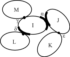
Figure II.1: Illustration of an example structure where five sub-units have been joined at four vertices $\alpha$, $\gamma$, $\delta$, $\epsilon$. Each sub-unit is illustrated by an ellipse where we associate the interior with the internal conformation of the scattering sites and the circumference with the reference points on the sub-unit. Sub-units are joined to each other by reference points, and they are illustrated as a single dot (e.g. $\epsilon$, $\delta$, $\gamma$) for a regular reference point or a thick line (e.g. $\langle\alpha\rangle$, $\langle\delta\rangle$) for distributed reference points. Note that we use the same Greek letter to label vertices in the structure, and regular or distributed reference points on different sub-units at the same vertex.

Here we write explicitly the reference points, that are to be averaged over in the form factor amplitudes and phase factors. Here and below we use $\langle\alpha\rangle$ to denote the case where the $\alpha$th reference point label on the $I$th sub-unit has been averaged. We continue to denote by $\alpha$ a regular reference point, where no average is to be performed. The formalism (eqs. II.4-II.6) remains valid when some or all form factor amplitudes and phase factors include distributed reference points.

Fig. II.1 schematically illustrates an example structure for which the formalism can provide the corresponding scattering expression. It shows how sub-units can be joined either at regular reference points or at distributed reference points. Note how a reference point is associated with a sub-unit, hence $\delta$ refers to a regular reference point on sub-unit $L$, that is joined to any of the $\delta$ reference points on the $I$th sub-unit denoted by the $\langle\delta\rangle$ average reference point. In general, a vertex have an arbitrary functionality, and a sub-unit can have an arbitrary number of reference points at which it can join with other sub-units. Hence the structures described by formalism is not limited to two-functional graph-like structures, but to any hyper-graph structures that does not contain loops.

In the special case, where we can make a one-to-one identification between reference points and scattering sites such that $n=i$, ${\bf R}_{I\alpha n}={\bf r}_{Ii}$, and $Q_{I\alpha n}=b_{Ii}/\beta_{I}$. Then II.7, II.2, II.8, and II.3 are identical to the form factor eq. II.1. Hence we conclude that $A_{I\langle\alpha\rangle}(q)=\Psi_{I\langle\alpha\rangle\langle\omega\rangle}(q)=F_{I}(q)$ in this case. For a polymer chain, for instance, this means that the form factor amplitude relative to a random position on the polymer, and the phase factor relative to two random positions on the polymer are identical to the polymer form factor. This is not a surprise since the site-to-site, site-to-reference point and reference-to-reference point pair-distance distributions all are identical in this case. When deriving form factors for a given structure, we often assume that all sites in a sub-unit has equal excess scattering length, hence all the known expressions for form factors of structures can be uses as reference point averaged form factor amplitudes and phase factors to describe structures with distributed link positions.

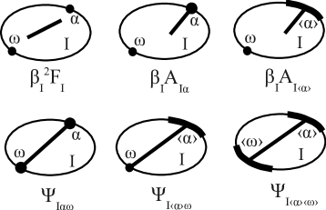
Figure II.2: Definition of diagrams representing the sub-unit form factor, form factor amplitude, and phase factor terms expressed for the different possibilities of reference point averages for the $I$th sub-unit.

Fig. II.2 introduces a diagrammatic interpretation of the form factor, form factor amplitude and phase factor of a sub-unit. As in fig. II.1 we associate each sub-unit with an ellipse, where reference points are associated with the circumference while the scattering sites are associated with the interior. The form factor is the Fourier transform of the pair-distance distribution between all scattering sites in a sub-unit, and we illustrate this by a straight line inside the sub-unit ellipse. Form factor amplitudes and phase factors depend on reference points. Regular reference points are shown as dots, while distributed reference points are illustrated as a thick line on the circumference. The form factor amplitude is Fourier transform of the pair-distance distribution between a specified reference point and all scattering sites inside the sub-unit, and this is illustrated as a line from dot to the inside of the sub-unit. In the case, of a reference point average, we illustrate the reference point not as a dot but by a thick line illustrating all the possible reference points, and the form factor amplitude as a line from anywhere along the thick line to the inside of the sub-unit. The phase factor is the Fourier transform of the pair-distance distribution between two specified reference points, and this is illustrated as a line traversing the sub-unit connecting two reference points or reference point averages.

Using eq. II.1, we can calculate the scattering form factor for a given structure composed of sub-units joined by regular or distributed reference points. The first term is just a sum over the form factors of all the sub-units weighted by their excess scattering lengths. The second term is more complicated, and it describes the scattering interference contributed by different sub-unit pairs. For each distinct pair of sub-units $I$ and $J$ in the double sum, we identify which vertex $\alpha$ at sub-unit $I$ that is nearest sub-unit $J$ and which vertex $\omega$ at sub-unit $J$ that is nearest to sub-unit $I$. Here “near” means in terms of the shortest path originating at a reference point $\alpha$ (or $\langle\alpha\rangle$) on $I$ and terminating on a reference point $\omega$ (or $\langle\omega\rangle$) on $J$. We denote the path connecting $\alpha$ and $\omega$ through the structure $P(\alpha,\omega)$. For the product, we have to identify each sub-unit $K$ on this path and also identify the reference points $\tau$ and $\eta$ (or $\langle\tau\rangle$, $\langle\eta\rangle$) across which the sub-unit is traversed. For some structures the path can traverse a sub-unit by the same reference point. In the case of a well defined reference point $\Psi_{K\alpha\alpha}(q)\equiv 1$ and we can neglect the contribution, however in the case of an distributed reference point the corresponding term $\Psi_{K\langle\alpha\rangle\langle\alpha\rangle}(q)$ will contribute to the product. The path construction is always unique and well defined for structures that does not contain loops.

The form factor expression (eq. II.4) has a quite simple physical interpretation, despite the complex notation required to describe branched reference point distributed structures. The structural form factor is the pair-correlation function between all scattering sites in the structure. It can be obtained by propagating position information between all scattering sites in the structure. When both sites belong to the same sub-unit it is given by the sub-unit form factors and is described by the first term in eq. II.4. The distance information between sites on different sub-units is obtained by propagating position information along paths through the structure. To propagate site-to-site position information between sites in sub-unit $I$ and sites in sub-unit $J$, we first have to propagate the position information between the sites in sub-unit $I$ to the vertex $\alpha$ at $I$. This is done by the form factor amplitude $\beta_{I}A_{I\alpha}$ or $\beta_{I}A_{I\langle\alpha\rangle}$. The position information is then propagated step-by-step along the path of intervening sub-units towards the vertex $\omega$ at sub-unit $J$. Each time a sub-unit is traversed it contributes a phase factor $\Psi_{K\tau\eta}$, $\Psi_{K\langle\tau\rangle\eta}$,$\Psi_{K\tau\text{$\langle$}\eta\rangle}$, or $\Psi_{K\langle\tau\rangle\langle\eta\rangle}$ to account for the conformationally averaged distance between the two (potentially distributed) reference points. Finally the position information is propagated between the vertex $\omega$ and all the sites inside the $J$ sub-unit. This is done by the final form factor amplitude $\beta_{J}A_{J\omega}$ or $\beta_{J}A_{J\langle\omega\rangle}$. Only the amplitudes has an excess scattering length prefactor, since they represent the amplitudes of scattered waves from all the scatterers inside the sub-units relative to the $\alpha$ and $\omega$ vertices while the product of phase factors represent excess phase contributed by the path between the vertices. The product of all these propagators describe the scattering length weighted site-to-site scattering interference contribution from the $I$’th and $J$’th sub-units. By summing over all such pair contributions all the possible site-to-site pair-distances in the structure are accounted for.

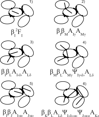
Figure II.3: Diagrammatic representation of some of the terms contributing to the form factor of the structure shown in fig. II.1 using the definition of diagrams shown in fig. II.2.

Fig. II.3 diagrammatically illustrates some of the terms that contributes to the form factor (eq. II.4) using the diagrammatic definitions in fig. II.2. We can generate all the diagrams by picking a pair of sites inside the same or two different sub-units and drawing a line between them using reference points to step between sub-units and to traverse across sub-units (diagram 1). A line between two sites within the same sub-unit contributes the form factor of that sub-unit. Sub-units that are joined directly to each other will contribute the product of two form factor amplitudes and excess scattering lengths of the two sub-units (diagram 2, 3, 5). For sub-units that are not directly joined to each other, the form factor amplitude product is further multiplied by the phase factors of all the sub-units on the intervening path (diagram 4, 6). For all the reference point labels of the form factors and phase factors, we either have a regular reference point, or a distributed reference point which depend on the details of the given structure. In general, for a structure of $N$ sub-units, there will be $N$ form factor contributions and $N(N-1)/2$ different scattering interference contributions that has to be determined. The longest possible path is $N-2$ sub-units which occurs in the case of a linear chain of sub-units.

Similar diagrammatic interpretations apply to the structural form factor amplitude and phase factors (eqs. II.5 and II.6). For the form factor amplitude we have to propagate position information between a specified vertex and all sites in the structure. Diagrammatically this can be done by picking a site in any sub-unit and drawing a line between the site and the specified vertex using reference points to step between sub-units and to traverse across sub-units. Summing over all the $N$ diagrams will produce the form factor amplitude of the structure. For the phase factor we have to propagate position information between two specified vertices. Diagrammatically this is done by drawing a line between the two vertices using reference points to step between sub-units and to traverse across sub-units. The resulting structural phase factor is the product of the phase-factors of all the intervening sub-units.

With the diagrammatic interpretation of the formalism, it becomes quite easy to draw a structure, and write down the corresponding scattering expressions. The price of this simplicity is that we had to assume that sub-units are mutually non-interacting, that the joints between sub-units are completely flexible, and that the structures does not contain loops. However, no assumptions were made about the internal structure of the sub-units. The formalism is complete in the sense that the three structural scattering expressions allows a whole structure to be used as a sub-unit to build more complex structures. This we utilized in Paper 1 but will not use here.Svaneborg and Pedersen (2012) The formalism is also generic in the sense that scattering contributions due to structural connectivity and the internal structure of the sub-units have been completely decoupled. This allows us to write down generic scattering expressions for structures without knowing what sub-units they are made of. This information can be specified at a later point when concrete expressions for the sub-unit form factor, form factor amplitudes, and phase factors are inserted. Below we give some generic examples, and then dedicate the rest of the paper to derive and present scattering expressions characterizing specific sub-unit structures.

II.1 Example structures

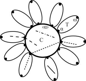
Figure II.4: Diagrammatic representation of the form factor of a block copolymer micelle with a core sub-unit “C” and a number of identical sub-units “T” tethered at random points on the surface. All the scattering contributions are shown using the diagrammatics in fig. II.2. They correspond to $\beta_{T}^{2}F_{T}$ (solid line), $\beta_{T}^{2}A_{T\alpha}^{2}\Psi_{C\langle\alpha\rangle\langle\alpha\rangle}$ (short dashed line), $\beta_{T}\beta_{C}A_{T\alpha}A_{C\langle\alpha\rangle}$ (long dashed line), and $\beta_{C}^{2}F_{C}$ terms (dot dashed line) in eq. II.9.

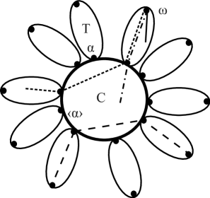
Figure II.5: Diagrammatic representation of the form factor amplitude and phase factor of a block copolymer micelle. The scattering contributions to $A_{mic,\omega}$ are shown by lines starting at an $\omega$ reference point on a tethered sub-unit and using the diagrammatics in fig. II.2. They correspond to the $\beta_{T}A_{T\omega}$ (solid line), $\beta_{C}A_{C\langle\alpha\rangle}\Psi_{T\omega\alpha}$ (dash dotted line), and $\beta_{T}A_{T\alpha}\Psi{}_{C\langle\alpha\rangle\langle\alpha\rangle}\Psi_{T\alpha\omega}$ terms (short dashed line) in eq. II.10. The phase factor (eq. II.11) between the tips of two tethered sub-units is given by $\Psi_{T\omega\alpha}^{2}\Psi_{C\langle\alpha\rangle\langle\alpha\rangle}$ (long dashed line) .

We can regard a micelle as $N$ identical two-functional sub-units tethered by one end to a random site on the surface of geometric structure representing the core. Such a structure is shown in fig. II.4. Note that the core surface still is referred to by a single reference point label $\alpha$. Similarly, we can regard a bottle-brush polymer as $N$ identical two-functional sub-units tethered by one end to a random point on a main structure such as a polymer chain. The connectivity of the two structures is identical, and hence they are characterized by the same generic scattering expression:

$$F_{mic}(q)=\left(N\beta_{T}+\beta_{C}\right)^{-2}\left(\beta_{C}^{2}F_{C}+N\beta_{T}^{2}F_{T}\right.$$

$$\left.+2N\beta_{C}\beta_{T}A_{C\langle\alpha\rangle}A_{T\alpha}+N(N-1)\beta_{T}^{2}A_{T\alpha}^{2}\psi_{C\langle\alpha\rangle\langle\alpha\rangle}\right)$$ (II.9)

Here the tethered sub-units are denoted by $T$ and the end attached to the core surface is denoted “$\alpha$” while “$\omega$” denotes the free end. The core sub-unit is denoted by $C$ and the average over random surface points is denoted by $\langle\alpha\rangle$. The form factor consists of terms representing all the possible pair distributions between sub-units in the structure. These are shown in fig. II.4. Each term has a prefactor which for form factor terms is the number of corresponding sub-units in the structure. The form factor amplitude product terms represent pair distributions between different sub-units and they are counted twice. Hence there is both an $A_{C\langle\alpha\rangle}A_{T\alpha}$ contribution and an identical $A_{T\alpha}A_{C\langle\alpha\rangle}$ contribution for each of the $N$ tethered sub-units. For the pair distribution between two tethered sub-units, we note that we have $N$ tethered sub-units to pick the starting point from, and $N-1$ tethered sub-units to pick end ending point. This also counts each pair twice. The prefactor of the form factor ensures it is normalized to unity in the limit of small $q$ values.

We have chosen to express the form factor amplitude relative to the tip of a tethered sub-unit. The form factor amplitude represents the pair distribution between the reference point at the tip of a tethered sub-unit and the sites in the same sub-unit, the sites in the core, and in the sites in the other tethered sub-units. These are shown in fig. II.5 and when taking into account the multiplicity of the sub-units the normalized form factor becomes

$$A_{mic,\omega}(q)=\left(N\beta_{T}+\beta_{C}\right)^{-1}\left(\beta_{C}\Psi_{T,\omega\alpha}A_{C,\langle\alpha\rangle}\right.$$

$$\left.+\beta_{T}A_{T\omega}+\beta_{T}(N-1)\Psi_{T\omega\alpha}\psi_{C\langle\alpha\rangle\langle\alpha\rangle}A_{T\alpha}\right).$$ (II.10)

The contribution to the tip-to-tip phase factor is also shown in fig. II.5 and is given by

$$\Psi_{mic,\omega\omega}(q)=\psi_{T\alpha\omega}^{2}\Psi_{C\langle\alpha\rangle\langle\alpha\rangle}.$$ (II.11)

Since exactly the same diagrams are required to describe a bottle-brush structure where side-structures are randomly tethered along some main chain structure (corresponding to the core of the micelle), the generic scattering expressions for these two structures are identical. They will first differ when we make choices of which sub-unit structures are involved and insert the corresponding form factor, form factor amplitudes, and phase factors in the expressions.

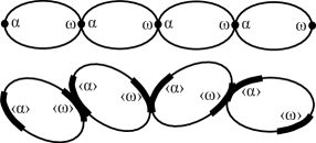
Figure II.6: Diagrammatic representation of chain of identical two-functional sub-units with regular reference points (top) or linked at two random positions (bottom).

PreviouslySvaneborg and Pedersen (2012), we derived the form factor of a chain of identical two functional sub-units using eq. II.4 as

$$F_{chain}(q)=\frac{F}{N}+2\frac{\Psi_{\alpha\omega}^{N}-N\Psi_{\alpha\omega}+N-1}{N^{2}(\Psi_{\text{$\alpha\omega$}}-1)^{2}}A_{\alpha}A_{\omega}.$$ (II.12)

Here we have discarded the superfluous sub-unit index, and also omitted the $q$ dependence on the right hand side for sake of brevity. A diagrammatic representation is shown in fig. II.6. $\alpha$ and $\omega$ denotes the two ends of the sub-unit. The sub-units can be asymmetric with regard to exchanging the two ends, for instance if the sub-unit is a di-block copolymer. The sub-units are joined as $\omega-\alpha$, leaving one free $\alpha$ end and one free $\omega$ end of the structure. If we assume that each of the reference points are picked from two distributions, then we obtain the scattering expression for the corresponding randomly joined chain by replacing the regular reference points by distributed reference points as

$$F_{chain}(q)=\frac{F}{N}+2\frac{\Psi_{\langle\alpha\rangle\langle\omega\rangle}^{N}-N\Psi_{\langle\alpha\rangle\langle\omega\rangle}+N-1}{N^{2}(\Psi_{\langle\alpha\rangle\langle\omega\rangle}-1)^{2}}A_{\langle\alpha\rangle}A_{\langle\omega\rangle}.$$ (II.13)

Fig. II.6 shows a diagrammatical representation of such a structure, where a random reference point $\omega$ is joined with a random reference point $\alpha$ on the next sub-unit. Again this leaves a structure with two ends characterized by $\langle\alpha\rangle$ and $\langle\omega\rangle$. If the sub-units are block-copolymers and the linking can be anywhere along the copolymer, then the corresponding structure is one where each polymer is randomly cross-linked with the previous and next polymers in the chain. Alternative, if the $\alpha$ link is anywhere in the $A$ block, and the $\omega$ link anywhere in the $B$ block, then the result will be a chain where each di-block copolymer (except for the ends) has one link on the each of the two blocks. These different choices correspond to different expressions for $\Psi_{\langle\alpha\rangle\langle\omega\rangle}$, $A_{\langle\alpha\rangle}$, and $A_{\langle\omega\rangle}$.

Note that the formalism is generic. We have made absolutely no assumptions as to the internal structure of the sub-units in the expressions above. These scattering expressions we have presented are completely generic and only encode the structural connectivity. The formalism is also complete, in the sense that a whole structure described by the formalism can be used as a sub-unit to build more complex structures within the formalism . For example, we can regard the three functions $F_{mic}(q)$, $A_{mic,\omega}(q)$, and $\Psi_{mic,\omega\omega}(q)$ given by eqs. II.9-II.11 as defining a micelle sub-unit. We could then obtain the scattering expression for a chain of micelles, by inserting the micelle sub-unit expressions into the form factor of a chain eq. II.12. This illustrates the versatility of the formalism.

III Sub-units with internal conformations

Each sub-unit is characterized by a three types of pair-distance distribution functions, the site-to-site, site-to-reference, and the reference-to-reference point pair-distribution functions, denoted $P_{ss}(\sigma,\rho;r)$, $P_{s\alpha}(\sigma;r)$, and $P_{\alpha\omega}(r)$, respectively. Here $\sigma$ and $\rho$ are running labels denoting scattering sites such as e.g. an index of a point scatterer or a contour-length, surface or volume element, respectively, while the $\alpha$ and $\omega$ labels denotes fixed reference points. The corresponding positions are denoted ${\bf r}_{\sigma}$, ${\bf r}_{\rho}$, ${\bf R}_{\alpha}$, and ${\bf R}_{\omega}$, respectively. In a rigid structure, the pair-distance $r=|{\bf r}_{\sigma}-{\bf r}_{\rho}|$ is constant and the pair-distance distributions reduce to delta functions. In a flexible structure with internal conformational degrees of freedom such as a polymer, the distance between two sites will in general be given by a distribution. Let the excess scattering length density of a scattering site $\sigma$ be denoted $b(\sigma)$, and $\beta=\int\mbox{d}\sigma b(\sigma)$ denotes the total excess scattering length of the sub-unit. The 3D isotropically averaged Fourier transform is $\mathcal{F}(P)=\int\mbox{d}r4\pi r^{2}\frac{\sin(qr)}{qr}P$. Hence the sub-unit scattering expressions are

$$F(q)=\beta^{-2}\int\mbox{d}\sigma\mbox{d}\rho b(\sigma)b(\rho)\int\mbox{d}r4\pi r^{2}\frac{\sin(qr)}{qr}P_{ss}(\sigma,\rho;r),$$ (III.1)

$$A_{\alpha}(q)=\beta^{-1}\int\mbox{d}\sigma b(\sigma)\int\mbox{d}r4\pi r^{2}\frac{\sin(qr)}{qr}P_{s\alpha}(\sigma;r),$$ (III.2)

$$\Psi_{\text{$\alpha\omega$}}(q)=\int\mbox{d}r4\pi r^{2}\frac{\sin(qr)}{qr}P_{\alpha\omega}(r).$$ (III.3)

In the case of a linear sub-unit with translational invariance along the contour, the pair-distance distributions functions only depend on the relative contour distance. Let $L$ denote the total contour length, such that $\sigma,\rho\in[0;L]$ denote a pair of sites along the sub-unit separated by a contour length distance $l=\text{|$\sigma$-$\rho$|}$ and a spatial separation $r$. The two ends are located at $\alpha=0$ and $\omega=L$, respectively. Then $P_{ss}(\sigma,\rho;r)=P(|\sigma-\rho|;r)$, $P_{s\alpha}(\sigma;r)=P(|\sigma-\alpha|;r)$, and $P_{\alpha\omega}(r)=P(|\alpha-\omega|;r)$ where $P(l;r)$ denotes the pair-distance distribution between two sites separated by a contour length $l$ and a direct distance $r$. In Appendix IX, we use these expressions to derive the form factor, form factor amplitudes, and phase factors of polymers, rods, and closed polymeric loops.

IV Scattering examples

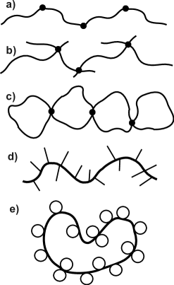
?figurename? IV.1: Illustration of chains and tethered structures. a) end-linked polymers, b) contour-linked polymers, c) contour-linked loops, d) rods contour-linked to a polymer, and e) loops contour-linked to a loop.

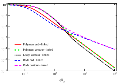
?figurename? IV.2: Normalized form factors from a chain of $N=100$ identical sub-units for end-linked polymers (red solid line), contour-linked polymers (green dashed), contour-linked polymer loops (blue dotted), end-linked rods (magenta short dashed), contour-linked rods (brown medium dashed). All sub-units has the same radius of gyration $R_{g}$.

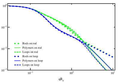
?figurename? IV.3: Normalised form factor for bottle brush structures where the main chain structure is either a rod (green) or a polymer loop (blue). The main chain structure has $N=20$ rods (dotted), polymers (solid), or polymer loops (dashed) tethered at random positions. The main chain and tethered sub-unit radii of gyration, $R_{g,C}$ and $R_{g}$, are fixed at $R_{g,C}/R_{g}=10$ for all the structures. The excess scattering length of the core and tethered sub-units are the same $\beta_{C}=\beta_{T}$.

Fig. IV.1 a-c illustrates some of the possible structures obtained by linking sub-units into chains. When identical polymers are end-linked the result is a long linear polymer. A very different structure is obtained, when polymers are allows to link anywhere along their contour. The result resembles a bottle-brush structure, where each sub-unit in the chain has two pendant chains of a random length. Note that just as in the end-linked case, all the internal sub-units in the contour-linked chain have exactly two links. This is very different from a truly randomly linked structure, which would form a gel-like network. The scattering from a gel-like network can be described by the Random Phase Approximation (RPA)Benoit and Benmouna (1984), and the diagrammatic representation of the RPA form factor corresponds to a weighed sum over contour-linked chain diagrams of varying number of sub-units.

The scattering from these structures are obtained from eq. II.13 by inserting the corresponding sub-unit form factor, form factor amplitude and phase factors. We have derived these terms for a flexible polymer chain, a rod, and a closed polymer loop in appendix IX. Fig. IV.2 shows the scattering from end-linked and contour-linked polymers and rods, as well as contour-linked loops. At small $q$ values we observe the Guinier $F(q)\approx 1+\frac{(qR_{g})^{2}}{3}$ regime, where $R_{g}$ is the radius of gyration of the entire structure, at intermediate $q$ values we see the power law characteristic of the fractal dimension of the structure, while at large $q$ values we see the scattering from the sub-units. The end-linked chain shows the expected Debye scattering behavior corresponding to a random walk with an asymptotic behavior $2(qR_{g}){}^{-2}$ at large $q$ values. The contour-linked polymers have a smaller radius of gyration since the chain structure is more at intermediate length scales, however at small length scales we again see the same sub-unit scattering as for the end-linked polymers. The chain of polymer loops is more compact than the chain of end-linked polymers, which is why their scattering is larger at large $q$ values, however at large $q$ values we observe the asymptotic $(qR_{g})^{-2}$ behaviour expected for a polymer loop. The end-linked chain of rods is observed to have the largest radius of gyration of all structures. At intermediate length scales the end-linked rod chain has a random-walk like structure, while at small length scales shows a cross-over to the $\pi(Lq)^{-1}$ asymptotic behavior characterizing the rod-like sub-units. Chains of contour-linked polymers, polymer loops, and rods have the same radius of gyration, since we have fixed the size of the sub-units to produce the same radius of gyration.

Fig. IV.1d-e shows the bottle-brush structures that are obtained by tethering rods to a long main chain polymer and by tethering polymer loops to a main chain polymer loop. The scattering from these structures is obtained from eq. II.9 by inserting the corresponding form factor, form factor amplitudes and phase factors of the main chain and tethered sub-units. The scattering form factors are shown in fig. IV.3. Again we have fixed the radius of gyration of the main chain and of the tethered sub-units to the same values independent of their structure and for this reason all the bottle-brush structures has the same radius of gyration. At intermediate length scales we see a small regime with power law behavior corresponding to the fractal dimension of the main chain $q^{-2}$ for the random-walk like polymer loop and $q^{-1}$ for the straight rod, while at small length scales we observe the power law corresponding to the fractal dimensions of the tethered sub-units. Again we observe that the polymer loop sub-unit scattering is a factor one half lower than that of the linear polymer sub-unit.

V Geometric sub-units

We assume that a sub-unit is a rigid geometric body without internal degrees of freedom. In this case, it is more convenient to express the sub-unit scattering expressions as the orientational average of the phase integral over all the scattering sites as

$$F_{rigid}(q)=\left\langle{\cal F}_{\beta}({\bf q},{\bf O}){\cal F}_{\beta}(-{\bf q},{\bf O})\right\rangle_{o},\quad A_{rigid}(q,{\bf O})=\left\langle{\cal F}_{\beta}({\bf q},{\bf O})\right\rangle_{o},$$ (V.1)

here $\left\langle\cdots\right\rangle_{o}$ denotes an orientational average. While the form factor is independent of the choice of origin ${\bf O}$, it is useful when expressing form factor amplitudes, since we have $A_{rigid,\alpha}(q)=A_{rigid}(q,{\bf R}_{\alpha})$ for a particular regular reference point ${\bf R}_{\alpha}$. The phase integral is defined as

$${\cal F}_{\beta}({\bf q},{\bf O})=\left(\int\mbox{d}{\bf r}\beta({\bf r})\right)^{-1}\int\mbox{d}{\bf r}\beta({\bf r})\exp\left(i\mathbf{q}\cdot(\mathbf{r}-\mathbf{O})\right),$$ (V.2)

which is the Fourier transform of the excess scattering length density distribution $\beta({\bf r})$ of the sub-unit relative to the origin ${\bf O}$. We normalize the phase integral such that ${\cal F}_{\beta}({\bf q}=0,{\bf O})=1$. The major challenge when calculating the scattering from geometric objects is to calculate the phase integral analytically and then perform the orientational averages.

Since we are not only interested in regular reference points, but also reference points that are averaged over distributions of potential reference point sites, we will focus on the situation where these site distributions are also characterized by a geometric objects. For instance, we could be interested in the form factor amplitude of a sphere relative to a random site on its surface, or the phase factor between two random sites on the surface of a sphere. By generalizing the averages eqs. (II.7 and II.8) into integrals over reference point distributions, and recognizing that these averages can be recast into the form of phase factor integrals, we can express the reference point distribution averaged form factor amplitude and phase factors as

$$A_{rigid\langle\alpha\rangle}(q)=\left\langle\int\mbox{d}{\bf r}^{\prime}Q_{\alpha}({\bf r}^{\prime}){\cal F}_{\beta}({\bf q};{\bf r}^{\prime})\right\rangle_{o}=\left\langle{\cal F}_{\beta}({\bf q},{\bf O}){\cal F}_{Q_{\alpha}}(-{\bf q},{\bf O})\right\rangle_{o},$$ (V.3)

$$\Psi_{rigid\langle\alpha\rangle\omega}(q)=\left\langle\int\mbox{d}{\bf r}Q_{\alpha}({\bf r})e^{i{\bf q}\cdot({\bf r}-{\bf R}_{\omega})}\right\rangle_{o}=\left\langle{\cal F}_{Q_{\alpha}}({\bf q},{\bf R}_{\omega})\right\rangle_{o},$$ (V.4)

and

$$\Psi_{rigid\langle\alpha\rangle\langle\omega\rangle}(q)=\left\langle\int\mbox{d}{\bf r}\mbox{d}{\bf r}^{\prime}Q_{\alpha}({\bf r})Q_{\omega}({\bf r}^{\prime})e^{i{\bf q}\cdot({\bf r}-{\bf r}^{\prime})}\right\rangle_{o}=\left\langle{\cal F}_{Q_{\alpha}}({\bf q},{\bf O}){\cal F}_{Q_{\omega}}(-{\bf q},{\bf O})\right\rangle_{o}.$$ (V.5)

Here ${\cal F}_{Q_{\alpha}}({\bf q},{\bf O})$ denotes the Fourier transform (eq. V.2) of the reference point site probability distribution $Q_{\alpha}({\bf r})$. The form factor amplitude $A_{\langle\alpha\rangle}(q)$ and double averaged phase factor $\Psi_{\langle\alpha\rangle\langle\omega\rangle}(q)$ are independent of the choice of origin ${\bf O}$ by construction. Again we recognize that if the normalized excess scattering length distribution and the reference point site probability distribution are proportional $\beta({\bf r})\propto Q_{\alpha}({\bf r})$, then the form factor, averaged form factor amplitude, and double averaged phase factor reduce to the same function. Finally, the phase factor between two regular reference points ${\bf R}_{\alpha}$ and ${\bf R}_{\omega}$ is given by

$$\Psi_{rigid,\alpha\omega}(q)=\frac{\sin(q|\mathbf{R}_{\alpha}-\mathbf{R}_{\omega}|)}{q|\mathbf{R}_{\alpha}-\mathbf{R}_{\omega}|}.$$ (V.6)

For a large number of geometric objects the scattering form factor is known, see e.g. Pedersen (2002). In an appendix, we derive the scattering expressions characterizing spheres, flat disks, spheres, and cylinders with special emphasis on how phase factors and form factor amplitudes change depending on different choices of reference point distributions. This is relevant in many applications e.g. for structures such as block-copolymer micelles and polymer brushes end-grafted to a surface or an interface.Pedersen and Gerstenberg (1996); Pedersen (2000) Below we give some examples.

VI Scattering examples

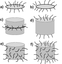
?figurename? VI.1: Illustration of tethering geometries: a) disk surface, b) disk rim, c) cylinder equator, d) end, e) side, and f) surface tethering.

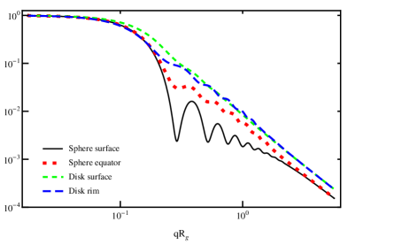
?figurename? VI.2: Normalized form factors for spherical core sub-unit with $N=100$ polymers tethered on the surface (black solid line), at the equator (red dotted line), and for a disk-like core sub-unit with polymers tethered on the surface (green short dashed line) and on the rim (blue long dashed line). The sub-units has the same radii of gyration with $R_{g,C}/R_{g}=10$, and the excess scattering lengths $\beta_{C}=100\beta_{T}$ .

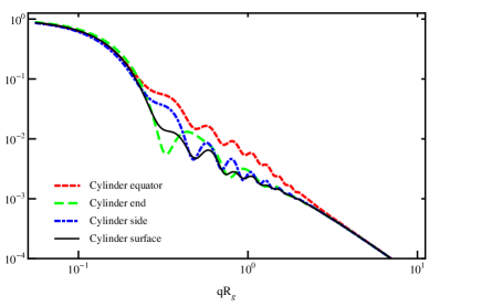
?figurename? VI.3: Normalized form factors of cylinders with $N=100$ polymer sub-units for equator (black solid line), end (red dotted line), side (green short dashed line), and surface (blue long dashed line) tethering geometries. The sub-units has fixed radii of gyration with $R_{g,C}/R_{g}=10$, the length $L$ and radius $R$ of the cylinder are equal, and the excess scattering lengths are $\beta_{C}=100\beta_{T}$.

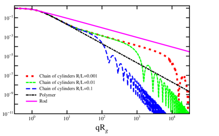
?figurename? VI.4: Normalised form factors for chains of $N=100$ cylinders as function of their aspect ratio for $R/L=0.001$ (red dotted line), $0.01$ (green short dashed), $0.1$ (blue long dashed). Also shown are the scattering from a polymer (black dot-dashed) and a rod (magenta solid line). The horizontal axis of each form factor has been scaled with the radius of gyration of each of the structures.

Fig. VI.1 shows some of the possible tethering geometries for disk-like and cylindrical micelles. For a disk we can either have the sub-units tethered to anywhere on the surface, or only at the rim of the surface. For a cylinder we could for instance tether polymers to the equator, the two ends, the side, or the entire surface of the cylinder. The corresponding scattering expressions are obtained from eq. II.9 by inserting the form factor, form factor amplitudes, and phase factors corresponding to the chosen sub-units and tethering geometry. In Appendix X, we have derived the required expressions to characterize these tethering geometries.

Fig. VI.2 shows the form factors for disk-like and spherical micelles. At small $q$ values we observe the Guinier regime which characterizes the radius of gyration of the whole structure, while at large $q$ values we observe the scattering due to the tethered chain sub-unit. In an intermediate regime, the scattering is both due to the micellar core geometry and the tethered sub-units. Even though the number of chains is the same, significant differences are observed in the scattering for the different tethering geometries, but coincidentally the sphere with equatorial tethering and disk with rim tethering produce very similar scattering patterns. Fig. VI.3 shows the form factors for cylindrical micelles for different choices of tethering geometry. Again the tethering geometry is observed to introduce significant differences in the spectra.

The scattering expression for a chain of thick end-linked cylinders are obtained from eq. II.12 by inserting the form factor, form factor amplitude relative to the reference point where the axis crosses the end, and phase factor between the two ends. In fig. VI.4, the scattering from this thick random walk is compared to that of a thin polymer and a rod. At large distances in the Guinier regime we see the crossover from a point like structure at the very largest scales to a random walk like structure with scaling behavior $(qR_{g})^{-2}$. At intermediate length scales the cylinder structure is probed and shows a scaling behavior like $(qL)^{-1}$ comparable to the rod. At length scales at and below the radius of the rod, we see strong oscillations due to cross section of the cylinder, and the envelope of the scattering curve shows the $q^{-4}S^{2}$ behavior of Porod scattering from the surface, where $S$ denotes the total surface area of the cylinders.

VII Conclusions

In a previous paperSvaneborg and Pedersen (2012), we presented a formalism for predicting the scattering from a linear and branched structures composed of mutually non-interacting sub-units. A sub-unit can have an arbitrary number of reference points. Sub-units are connected into structure by joining their reference points to the reference points of other sub-units. In the present paper, we have briefly presented the formalism, and generalized it to the case where reference points can be characterized by a distribution of potential link positions on a sub-unit. For instance, one reference point of a polymer could be a random site along the contour, or a reference point of a sphere could be a random point on the surface. To generalize the formalism, we had to assume that reference point distributions on different sub-units are mutually statistically uncorrelated.

We used the generalized formalism to derive the generic scattering expression for a micelle / bottle-brush structure with a core sub-unit and a number of identical sub-units tethered to random positions on the core / main chain. Since the connectivity of a micelle and a bottle-brush is the same, the generic scattering expressions are also identical. We presented the general scattering expressions for the form factor, form factor amplitudes and phase factors of a structure with internal conformations. We illustrated the scattering the expression using end-linked and contour-linked chains of polymers, rods, and polymeric loops and bottle-brush structures of rods and polymer loops with tethered polymers, rods, or polymer loops. All these structures are special cases of the generic scattering expression, which are obtained when the form factor, form factor amplitudes, and phase factors of the corresponding sub-units are inserted into the generic structural scattering expression. We derived these terms in an appendix.

We also presented the general expressions for the form factor, form factor amplitudes, and phase factors for rigid sub-units without internal conformations. We derived the scattering terms for spheres, disks, and cyllinders for a variety of different reference point distributions in an appendix. While the form factors for all these sub-units are known, the form factor amplitudes and phase factors are not necessarily known, and these are required by the formalism. This allowed us to predict the scattering from micelles with different core structures and geometries of tethering the corona sub-units.

Taken together, the formalism presented in ref. Svaneborg and Pedersen (2012), the present generalization to distributed reference points, and the sub-unit scattering expressions derived in the appendix enables the scattering from a large class of regular or random-linked, homogeneous or heterogeneous, linear and branched structures to be derived with great ease. With this, we hope to have provided a valuable tool for analyzing scattering data in the future.

VIII Acknowledgments

C.S. and J.S.P. gratefully acknowledges discussions with C.L.P. Oliveira. Funding for this work is provided in part by the Danish National Research Foundation through the Center for Fundamental Living Technology (FLinT). The research leading to these results has received funding from the European Community’s Seventh Framework Programme (FP7/2007-2013) under grant agreement n° 249032, MatchIT - Matrix for Chemical IT.

IX Appendix: Sub-units with internal conformations

In the following we derive the scattering expressions for rigid rods, flexible polymers, and closed polymer loops using eqs. III.1-III.3.

IX.1 Rigid rods

The most basic example is a randomly orientated infinitely thin rigid rod of length $L$. The rigid rod is special as the contour length $l$ and direct distance $r$ between a pair sites are degenerate parameters, hence the $\delta(r-l)$ factor in the rod pair-distance distribution: $P(l;r)=\delta(r-l)\Theta(L-r)/(4\pi l^{2})$, where $\Theta(x)$ denotes the Heaviside step function. Performing the contour length integrations (III.1)-(III.3), the rod scattering triplet becomes

$$F_{rod}(q,L)=\frac{2\mbox{Si}(x)}{x}-\frac{4}{x^{2}}\sin^{2}\left(\frac{x}{2}\right),$$ (IX.1)

$$A_{rod}(q,L)=\frac{\mbox{Si}(x)}{x}\quad\Psi_{rod}(q,L)=\frac{\sin(x)}{x},$$ (IX.2)

where $x=qL$ and $\mbox{Si}(x)=\int_{0}^{x}\mbox{d}y\sin(y)/y$ is the Sin integralAbramowitz and Stegun (1964). The expression for the rod form factor was previous derived by NeugebauerNeugebauer (1953) and Teixera et al Teixeira et al. (2007). In the case where the reference points are distributed along the rod contour with a constant probability (denoted contour-linking and shown with sub-script $\langle c\rangle$ and $\langle c\rangle\langle c\rangle$), the rod phase factor and form factor amplitudes are given by

$$\Psi_{rod,\langle c\rangle\langle c\rangle}(q)=A_{rod,\langle c\rangle}(q)=F_{rod}(q,L).$$

IX.2 Flexible polymers

Flexible polymers can be modeled as random walks with a effective step length or Kuhn length $b$. The pair-distance distributions between two sites separated by a contour length $l$ are given by the Gaussian distribution

$$P_{rw}(l;r)=\left(\frac{3}{2\pi bl}\right)^{\frac{3}{2}}\exp\left(-\frac{3}{2}\frac{r^{2}}{bl}\right)$$

Inserting this distribution into eqs. (III.1)-(III.3) yields the scattering triplet characterizing a flexible polymer

$$F_{pol}(x)=\frac{2[e^{-x}-1+x]}{x^{2}},\quad A_{pol}(x)=\frac{1-e^{-x}}{x},\quad\mbox{and}\quad\Psi_{pol}(x)=e^{-x}$$ (IX.3)

here $x=(qR_{g,rw})^{2}$, and the radius of gyration is given by $R_{g,rw}^{2}=bL/6$. The result for the form factor amplitude has previously been given by Hammouda Hammouda (1992) and the form factor was calculated by Debye Debye (1947). These expressions can also be obtained as a self-consistency requirement of this formalism requiring that the scattering form factor, form factor amplitude and phase factor from a di-block copolymer with two identical blocks of length $L/2$ match the scattering expressions for one block of length $L$.Svaneborg and Pedersen (2012) Expressions for the scattering from poly disperse flexible polymer characterized by a Schultz-Zimm distribution are given in Ref. Benoit and Hadziioannou (1988). In the case where the reference points are distributed randomly along the polymer contour (denoted $\langle c\rangle$ and $\langle c\rangle\langle c\rangle$), the polymer phase factor and form factor amplitude are given by

$$\Psi_{pol,\langle c\rangle\langle c\rangle}(x)=A_{pol,\langle c\rangle}(x)=F_{pol}(x).$$

IX.3 Polymer loops

While the formalism does not apply for structures that contains loops, no assumptions are made as to the internal structure of the sub-units, which can contain loops. The simplest loop is formed by linking the two ends of a flexible polymer chain. We can model a polymer loop as two random walks with contour lengths $l$ and $L-l$, respectively, starting at ${\bf R}_{\alpha}$ and ending at the link $\mathbf{R}_{\omega}$. In this case, the pair-distance distribution is given by

$$P_{loop}(l;|\mathbf{R}_{\omega}-\mathbf{R}_{\alpha}|)\propto P_{rw}(l;|\mathbf{R}_{\omega}-\mathbf{R}_{\alpha}|)P_{rw}(L-l;|\mathbf{R}_{\omega}-\mathbf{R}_{\alpha}|),$$

and the corresponding phase factor becomes

$$\Psi_{loop,\alpha\omega}(q;l)=\exp\left(-\frac{bl(L-l)q^{2}}{6L}\right).$$

Since the link at $l$ can be anywhere along the loop $[0;L]$, we need to average over the link position to get the loop scattering:

$$\Psi_{loop,\langle\alpha\rangle\langle\omega\rangle}(q)=\int_{0}^{L}\frac{\mbox{d}l}{L}\Psi_{loop}(q;l)=\frac{\exp\left(-2y^{2}\right)D[y]}{y}.$$

Here $y=q\sqrt{bL}/\sqrt{24}$ and $D[y]=\exp(-y^{2})\int_{0}^{y}\exp(t^{2})dt$ is the Dawson integral, which is related to the imaginary part of the complex error functionAbramowitz and Stegun (1964). By construction, the form factor amplitude, form factor and average phase factor are all identical when the reference point(s) is averaged over all sites in the structure, since eqs. (III.1)-(III.3) become identical $A_{loop,\langle\alpha\rangle}(q)=F_{loop}(q)=\Psi_{loop,\langle\alpha\rangle\langle\omega\rangle}(q)$. The form factor of a flexible polymer loop was previous derived by Zimm and Stockmayer.Zimm and Stockmayer (1949)

X Appendix: geometric sub-units

Below we will derive the scattering from a solid sphere, a flat disk, and a cylinder for a variety of reference point distributions using eqs. V.1-V.5.

X.1 Solid sphere

For a solid homogeneous sphere with excess scattering length density $\beta$, we can characterize any scattering site by its spherical coordinate $\sigma=(r,\phi,\theta)$. Then $\mathbf{r}(\sigma)=(r\cos\phi\sin\theta,r\sin\phi\sin,r\cos\theta)$. We can choose a coordinate system such that the sphere center is located at the origin ${\bf O}=0$. Due to the spherical symmetry the scattering vector $\mathbf{q}$ is pointing towards the pole ($\theta=0)$, then $\mathbf{q}\cdot\mathbf{r}_{\sigma}=qr\cos\theta$. The phase integral becomes

$${\cal F}_{sphere}({\bf q},0;R)=\left(\frac{4\pi R^{3}}{3}\right)^{-1}\int_{-\pi}^{\pi}\mbox{d}\phi\int_{-1}^{1}\mbox{d}\cos\theta\int_{0}^{R}\mbox{d}rr^{2}e^{iqr\cos\theta}$$

$$=\frac{3\left(\sin(qR)-qR\cos(qR)\right)}{(qR)^{3}},$$ (X.1)

Due to the spherical symmetry, we do not need to perform an additional orientational average $\langle\cdots\rangle_{o}$ when using eqs. V.1-V.6. Hence, the form factor, the form factor amplitude and phase factor of a solid sphere with $\mathbf{R}_{\alpha}=\mathbf{R}_{\omega}=0$ fixed at the center (denoted subscript “c”) are given by

$$F_{sphere}(q;R)=A_{sphere,c}^{2}(q;R),$$ (X.2)

$$A_{sphere,c}(q;R)=\frac{3\left(\sin(qR)-qR\cos(qR)\right)}{(qR)^{3}},$$

$$\Psi_{sphere,cc}(q)=1.$$ (X.3)

The scattering from a solid sphere was derived by Reyleigh in 1911Rayleigh (1911). Having the reference points at the center is the simplest choice, however, for the derivation of e.g. the scattering from spherical micelles it is more relevant let the surface of the sphere be a reference point. In this case the corresponding normalized reference point distributions are $Q_{\alpha}({\bf R})=Q_{\omega}({\bf R})=\delta(|{\bf R}|-R)/(4\pi R^{2})$ representing a spherical shell. We can calculate ${\cal F}_{shell}({\bf q},0;R)$ by integration of eq. V.2. However, since the shell corresponds to the upper limit of the radial integral in eq. X.1, we can trivially obtain its Fourier transform by differentiation of ${\cal F}_{sphere}$ as

$${\cal F}_{shell}({\bf q},0;R)=\left(4\pi R^{2}\right)^{-1}\frac{\mbox{d}}{\mbox{d}R}\left[\frac{4\pi R^{3}}{3}{\cal F}_{sphere}({\bf q},0,R)\right]=\frac{\sin qR}{qR}.$$ (X.4)

Here we have introduced an area and volume prefactor to account for the normalizations of the two Fourier transforms, such that ${\cal F}_{shell}\rightarrow 1$ when $q\rightarrow 0$. We can obtain the form factor amplitude and phase factors relative to the surface reference point (denoted by subscript “$\langle s\rangle$”) combining eqs. X.1, X.4, V.3, and V.5 as

$$A_{sphere,\langle s\rangle}(q,R)=\frac{3\left(\sin(qR)-qR\cos(qR)\right)}{(qR)^{3}}\times\frac{\sin(qR)}{qR},$$

and

$$\Psi_{sphere,\langle s\rangle\langle s\rangle}(q,R)=\left(\frac{\sin(qR)}{qR}\right)^{2}.$$ (X.5)

The spherical phase factor was previously derived by Pedersen and Gerstenberg.Pedersen and Gerstenberg (1996)

X.2 Flat circular disk

Due to rotational symmetry, we can choose a geometry where the disk is in the $xy$ plane, and $\mathbf{q}$ in the $xz$ plane. Expressing the scattering site in polar coordinates $\sigma=(r,\phi)$, such that $\mathbf{r}=(r\cos\phi,r\sin\phi,0)$, and $\mathbf{q}=(q\sin\theta,0,q\cos\theta)$ then $\mathbf{q}\cdot\mathbf{r}=qr\cos\phi\sin\theta$.

$${\cal F}_{disk}({\bf q},0;R)=\frac{2J_{1}(qR\sin\theta)}{qR\sin\theta}$$ (X.6)

Expressing the integrals in cylindrical coordinates immediately provides the form factor, form factor amplitude and phase factor for $\mathbf{R}_{\alpha}=\mathbf{R}_{\omega}=0$ fixed at the center as

$$F_{disk}(q)=\left\langle\left(\frac{2J_{1}(qR\sin\theta)}{qR\sin\theta}\right)^{2}\right\rangle_{o}=\frac{2}{q^{2}R^{2}}\left[1-\frac{J_{1}(2qR)}{qR}\right],$$

$$A_{disk,c}(q)=\left\langle\frac{2J_{1}(qR\sin\theta)}{qR\sin\theta}\right\rangle_{o},\quad\Psi_{disk,cc}(q)=1$$ (X.7)

Here $J_{n}(x)$ denotes the $n$’th Bessel function of the first kindAbramowitz and Stegun (1964), and $\langle\cdots\rangle_{o}=\frac{1}{2}\int_{-1}^{1}\mbox{d}\cos(\theta)\cdots$ denotes the remaining orientational average, which needs to be performed numerically. The form factor of a disk first derived by Kratky and PorodKratky and Porod (1949). We could also choose to put the reference point anywhere on the circular rim of the disk. In this case, we can again obtain the Fourier transform of the points on a circular rim ${\cal F}_{rim}$ by differentiation of ${\cal F}_{disk}$ as

$${\cal F}_{rim}({\bf q},0,R)=\left(2\pi R\right)^{-1}\frac{\mbox{d}}{\mbox{d}R}\left[\pi R^{2}{\cal F}_{disk}({\bf q},0,R)\right]$$

$$=J_{0}(qR\sin\theta)$$ (X.8)

The corresponding form factor amplitude of the disk relative to any site on the rim and the phase factor between two sites on the rim (denoted by subscript $\langle r\rangle$)

$$A_{disk,\langle r\rangle}(q)=\left\langle\frac{2J_{1}(qR\sin\theta)}{qR\sin\theta}\times J_{0}(qR\sin\theta)\right\rangle_{o},$$ (X.9)

$$\Psi_{disk,\langle r\rangle\langle r\rangle}(q)=\left\langle J_{0}^{2}(qR\sin\theta)\right\rangle_{o}.$$ (X.10)

If we instead chooses to put the two reference points at any point on the surface of the disk (again denoting an average surface reference point by $\langle s\rangle$), the result is again given by the disk form factor as we have seen previously:

$$A_{disk,\langle s\rangle}(q)=\Psi_{disk,\langle s\rangle\langle s\rangle}(q)=F_{disk}(q).$$ (X.11)

X.3 Solid cylinder

We can choose a cylinder with its center at the origin and the axis along $z$, the natural choice is to describe it with polar coordinates $\sigma=(r,\phi,z)$ such that $\mathbf{r}(\sigma)=(r\cos\phi,r\sin\phi,z)$ and we define $\mathbf{q}=(q\sin\theta,0,q\cos\theta)$ then $\mathbf{q}\cdot\mathbf{r}(\sigma)=qr\cos\phi\sin\theta+qz\cos\theta$. The phase integral becomes

$${\cal F}_{cyl}({\bf q},{\bf O};R,L)=\frac{4J_{1}(qR\sin\theta)\sin(\frac{qL}{2}\cos\theta)}{LRq^{2}\sin\theta\cos\theta}\times e^{-i\mathbf{q}\cdot\mathbf{O}}.$$ (X.12)

We have chosen to explicitly write the origin ${\bf O}$, since this will be required to calculate the form factor amplitude. With regular reference points at the ends of the cylinder axis $\mathbf{R}_{\alpha}=(0,0,-L/2)$ and $\mathbf{R}_{\omega}=(0,0,+L/2)$ (denoted by subscript “$a$”), the form factor, form factor amplitude and phase factor can be derived as

$$F_{cyl}(q;R,L)=\left\langle\left(\frac{4J_{1}(qR\sin\theta)\sin(\frac{qL}{2}\cos\theta)}{LRq^{2}\sin\theta\cos\theta}\right)^{2}\right\rangle_{o},$$ (X.13)

$$A_{cyl,a}(q;R,L)=\left\langle{\cal F}_{cyl}({\bf q},{\bf R}_{\alpha};R,L)\right\rangle_{o}=\left\langle{\cal F}_{cyl}({\bf q},{\bf R}_{\omega};R,L)\right\rangle_{o}$$ (X.14)

$$=\left\langle\frac{4J_{1}(qR\sin\theta)\sin(\frac{qL}{2}\cos\theta)}{LRq^{2}\sin\theta\cos\theta}\cos\left(\frac{qL}{2}\cos\theta\right)\right\rangle_{o},$$ (X.15)

$$\Psi_{cyl,aa}(q;R,L)=\frac{\sin qL}{qL}.$$ (X.16)

The form factor of a solid cylinder was previously derived by FournetFournet (1951). We can also derive the Fourier transform of the end and side of the cylinder by differentiation as

$${\cal F}_{cyl,end}({\bf q},0;R,L)=\left(\pi R^{2}\right)^{-1}\frac{\mbox{d}}{\mbox{d}L}\left[\pi LR^{2}{\cal F}_{cyl}({\bf q},0;R,L)\right]$$

$$=\frac{2J_{1}(qR\sin\Theta)\cos(\frac{Lq}{2}\cos\Theta)}{qR\sin\Theta}$$ (X.17)

$${\cal F}_{cyl,side}({\bf q},0;R,L)=\left(2\pi RL\right)^{-1}\frac{\mbox{d}}{\mbox{d}R}\left[\pi LR^{2}{\cal F}_{cyl}({\bf q},0;R,L)\right]$$

$$=\frac{2J_{0}(qR\sin\Theta)\sin(\frac{Lq}{2}\cos\Theta)}{Lq\cos\Theta}$$ (X.18)

By combining eqs. X.17 and X.18 weighting the terms by their relative areas and normalizing, we obtain the Fourier transform of the surface of a cylinder asPedersen (2000)

$${\cal F}_{cyl,sur\!face}({\bf q},0;R,L)=(R+L)^{-1}\left(R{\cal F}_{cyl,end}+L{\cal F}_{cyl,side}\right)$$ (X.19)

With these Fourier transforms we can write down the form factor amplitudes and phase factors of the cylinder relative to a reference point distributed on the ends (denoted by subscript $\langle e\rangle)$, on the hull (denoted by $\langle h\rangle$) or anywhere on the surface (denoted by $\langle s\rangle$) as

$$A_{cyl,\langle e\rangle}(q;R,L)=\left\langle\frac{8J_{1}^{2}(qR\sin\theta)\sin(\frac{qL}{2}\cos\theta)\cos(\frac{Lq}{2}\cos\theta)}{LR^{2}q^{3}\sin^{2}\theta\cos\theta}\right\rangle_{o},$$

$$A_{cyl,\langle h\rangle}(q;R,L)=\left\langle\frac{8J_{0}(qR\sin\theta)J_{1}(qR\sin\theta)\sin^{2}(\frac{qL}{2}\cos\theta)}{RL^{2}q^{3}\sin\theta\cos^{2}\theta}\right\rangle_{o},$$

$$A_{cyl,\langle s\rangle}(q;R,L)=\left\langle\frac{4J_{1}(qR\sin\theta)\sin(\frac{qL}{2}\cos\theta)}{LRq^{2}\sin\theta\cos\theta}\right.$$

$$\left.\times\frac{2}{q(R+L)}\left(\frac{J_{1}(qR\sin\Theta)\cos(\frac{Lq}{2}\cos\Theta)}{\sin\Theta}+\frac{J_{0}(qR\sin\Theta)\sin(\frac{Lq}{2}\cos\Theta)}{\cos\Theta}\right)\right\rangle_{o},$$

$$\Psi_{cyl,\langle e\rangle\langle e\rangle}=\left\langle\left(\frac{2J_{1}(qR\sin\Theta)\cos(\frac{Lq}{2}\cos\Theta)}{qR\sin\Theta}\right)^{2}\right\rangle_{o},$$

$$\Psi_{cyl,\langle h\rangle\langle h\rangle}=\left\langle\left(\frac{2J_{0}(qR\sin\Theta)\sin(\frac{Lq}{2}\cos\Theta)}{Lq\cos\Theta}\right)^{2}\right\rangle_{o},$$

and

$$\Psi_{cyl,\langle s\rangle\langle s\rangle}=\left\langle\frac{4}{q^{2}(R+L)^{2}}\left(\frac{J_{1}(qR\sin\Theta)\cos(\frac{Lq}{2}\cos\Theta)}{\sin\Theta}\right.\right.$$

$$\left.\left.+\frac{J_{0}(qR\sin\Theta)\sin(\frac{Lq}{2}\cos\Theta)}{\cos\Theta}\right)^{2}\right\rangle_{o}.$$