Chaos in fluid dynamics Dynamical systems methods Pattern formation in reactions with diffusion, flow and heat transfer

Invariant barriers to reactive front propagation in fluid flows

Abstract

We present theory and experiments on the dynamics of reaction fronts in two-dimensional, vortex-dominated flows, for both time-independent and periodically driven cases. We find that the front propagation process is controlled by one-sided barriers that are either fixed in the laboratory frame (time-independent flows) or oscillate periodically (periodically driven flows). We call these barriers burning invariant manifolds (BIMs), since their role in front propagation is analogous to that of invariant manifolds in the transport and mixing of passive impurities under advection. Theoretically, the BIMs emerge from a dynamical systems approach when the advection-reaction-diffusion dynamics is recast as an ODE for front element dynamics. Experimentally, we measure the location of BIMs for several laboratory flows and confirm their role as barriers to front propagation.

Many dynamical systems are characterized by the propagation of fronts that separate distinct phases, including chemical reactions [1], plankton blooms [2], plasmas [3], epidemics [4], and flame fronts. Fronts propagating in non-advecting reaction-diffusion (RD) systems, i.e., with no fluid flow, have been the subject of much research. For instance, front speeds in the RD regime are well described by the existing Fisher-Kolmogorov-Petrovsky-Piskonuv (FKPP) theory [5, 6]. However, many real systems over a broad range of length scales exhibit coherent fluid or fluid-like motion that dramatically impacts front propagation, e.g., plankton blooms in ocean currents [7], or chemical reactions in microfluidic devices [8]. Despite the importance of flows in front-producing systems, a general framework for understanding their effect is lacking. Notably, attempts to extend FKPP theory through the use of an enhanced diffusivity have been shown inadequate in describing front propagation in laminar advection-reaction-diffusion (ARD) systems [9]. This suggests that we approach the problem from a different perspective.

In this Letter, through both theory and experiment, we reveal fundamental geometric structures that govern front propagation in two-dimensional (2D) flows. We draw inspiration from the theory of chaotic advection, which emphasizes the key role played by invariant manifolds as barriers to passive transport [10, 11]. The central idea of this Letter is that analogous manifolds—what we call burning invariant manifolds (BIMs)— serve as one-sided barriers to front propagation.

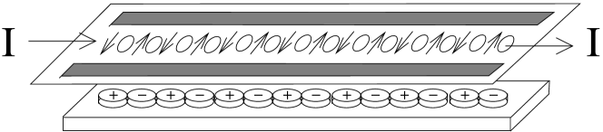
Figure 1: Exploded view of magnetohydrodynamic forcing. Current interacts with alternating magnets to produce a flow composed of a chain of alternating vortices. The fluid channel measures 1.9 cm x 27 cm.

We shall first consider a chain of alternating quasi-2D vortices (fig. 1), considering both a time-independent flow and a time-periodic flow with vortices that oscillate laterally. Both of these experiments are complemented by qualitative theoretical models. Finally we shall demonstrate the applicability of the proposed concepts in the more general setting of a spatially disordered flow (fig. 8).

Vortex chains provide a suitable context to introduce our geometric approach to front propagation, since much is already known about passive transport in these systems. Previous studies in both time-independent and time-periodic flows have found long-range passive transport that is often diffusive with a variance that grows linearly in time [12, 13, 14]. For the time-periodic flow, passive transport has been successfully analyzed [13, 14] in terms of invariant manifolds and the lobes [15, 16, 11] formed by their intersections. Reactive front propagation in this flow has also been experimentally studied [9, 17]. For the time-periodic flow, fronts often mode-lock to the external forcing [18, 9], propagating an integer number of vortex pairs in an integer number of drive periods. Importantly, this result contradicts any FKPP-type analysis that predicts front speeds that grow monotonically with enhanced diffusivity.

The vortex chain is generated (fig. 1) using a magnetohydrodynamic forcing technique [14]: an electric current passing through a thin (2 mm) conducting fluid interacts with a field produced by an alternating pattern of 1.9 cm diameter magnets below the fluid. Two strips of plastic define the fluid channel. The result is a chain of 14 vortices, each with width and height of $D=1.9$ cm. The flow can be made time-periodic by oscillating the magnets laterally, causing the vortices to oscillate likewise. The timescale of magnet oscillation is much longer than the viscous diffusion time ($\sim$ 4 s), which is a characteristic relaxation time for velocity fluctuations in the fluid layer. The spatially disordered flow (fig. 8a) is similarly generated, except the plastic strips are removed and the magnets are replaced by a disordered 2D configuration of smaller (0.6 cm) magnets.

The fluid for all experiments is composed of the chemicals for the excitable, ferroin-catalyzed, Belousov-Zhabotinsky (BZ) reaction [19]. The fluid is initially orange; insertion of a silver wire triggers a green reaction that propagates through the fluid. The reacting fluid is imaged from above with a CCD video camera. The front propagation speed is $V_{0}=0.007$ cm/s in the absence of a flow. In the theory, we assume the sharp front limit (consistent with the experiments), meaning the reaction proceeds rapidly compared to diffusion. We also assume that the chemical reaction has negligible feedback on the fluid flow.

We accompany these vortex chain experiments with theoretical computations using the following 2D fluid velocity field [12],

$$u_{x}(x,y,t) =+\sin(\pi[x+b\sin(\omega t)])\cos(\pi y),$$ (1)

$$u_{y}(x,y,t) =-\cos(\pi[x+b\sin(\omega t)])\sin(\pi y),$$

where $0\leq y\leq 1$, and $b\equiv B/D$, and $\omega\equiv\Omega D/U$ are dimensionless parameters with $U$, $\Omega$, and $B$ the (dimensional) maximum fluid speed, driving frequency, and driving amplitude, respectively ($b=B=0$ for a time-independent flow). This model has free-slip boundary conditions (BCs). While the experimental flow has no-slip BCs, it attains velocities comparable to the free-slip model within 1 mm of the wall. Also, Ekman pumping [20] in our experiments produces a weak 3D secondary flow that is not included in the model. Nevertheless, this model captures the basic features of the experimental flow and, in fact, has been successfully used to model both passive transport and mode-locking of reaction fronts for previous experiments  [12, 13, 18, 9].

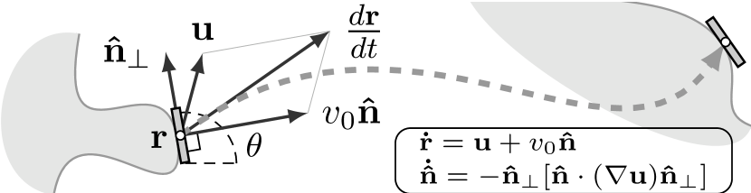
Figure 2: Each reaction front element independently propagates forward under advection ($\mathbf{u}$) and burning ($v_{0}\mathbf{\hat{n}}$). These 4D vector equations reduce to the 3D ODE eq. (2).

Previous theoretical studies of ARD in a vortex chain  [18, 21] utilized an Eulerian-grid-based computation. In contrast, we directly model the dynamics of the front between reactant and product using the following 3D ODE  (fig. 2),

$$\displaystyle\dot{x} =u_{x}+v_{0}\sin{\theta},\quad\quad\quad\dot{y}=u_{y}-v_{0}\cos{\theta},$$ (2a)

$$\displaystyle\dot{\theta} =-2u_{x,x}\sin{\theta}\cos{\theta}-u_{x,y}\sin^{2}{\theta}+u_{y,x}\cos^{2}{\theta},$$ (2b)

where $\mathbf{r}=(x,y)$ is the position of an infinitesimal front element, $\theta$ is the local orientation of the front, defined with respect to the $x$-axis, $\mathbf{u}(x,y,t)$ is the prescribed incompressible fluid velocity field, and $v_{0}\equiv V_{0}/U$ is the dimensionless burning speed. The 3D ODE can also be expressed in vector form, as shown in fig. 2. These ODEs assume that the front propagation speed is constant in the local fluid frame and does not depend on the local curvature of the front [23].

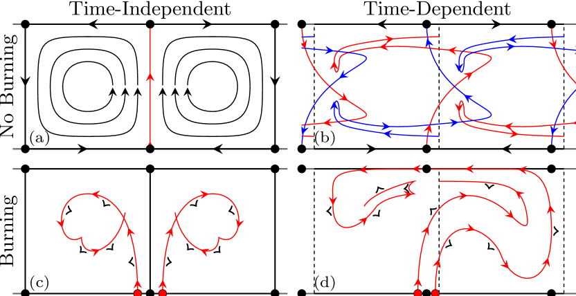
Figure 3: Schematics showing the geometric structures that govern passive transport and front propagation. Black arrows indicate fluid velocity. Blue/red denote stable/unstable manifolds. Black dots denote fixed points of 2D fluid flow. Red dots denote burning fixed points of eq. (2). Arrows tangent to unstable manifolds show unstable direction; normal wedge shapes show the “burning” direction $\mathbf{\hat{n}}$ of BIMs.

We investigate four physical regimes (fig. 3), the first two of which review existing theory, while the latter two introduce BIMs, their measurement, and their function.

Time-independent fluid flow, passive mixing (fig. 3a): Advection in a regular (integrable) flow is the base case. Here, the streamlines are closed, forming invariant tori. The stable and unstable invariant manifolds, anchored to hyperbolic fixed points on the top and bottom of the channel, are degenerate with one another and form separatrices, dividing the channel into isolated vortex cells.

Time-periodic fluid flow, passive mixing (fig. 3b): Mixing in the time-periodic flow is typically chaotic [12, 13, 14]; consequently, the dynamics are now best studied by a Poincaré map which advects a given $(x,y)$ position forward over one driving period. The separatrices from the time-independent case split into separate stable and unstable invariant manifolds, each attached to one hyperbolic fixed point on the channel wall. Lobes formed from the intersections of these complicated curves govern passive transport between neighboring vortices in the flow [11, 13, 14, 15, 16].

Time-independent fluid flow, reactive front propagation (fig. 3c): The addition of burning ($v_{0}\neq 0$) results in a few critical changes, central to this Letter. First, each advective hyperbolic fixed point in fig. 3a splits into two burning fixed points (fixed points of eq. 2), one on either side. Each burning fixed point lives in $xy\theta$-space, and so is endowed with a burning direction. These occur where the fluid velocity is exactly balanced by the burning velocity of the front. In our model, these points lie on the channel wall, while in our experiments, they lie roughly 1 mm away due to the no-slip BC. Each of these burning fixed points has one unstable and two stable directions, generating one-dimensional unstable manifolds – the burning invariant manifolds (BIMs) shown in fig. 3c. It is critical to recognize that each BIM has a burning direction, denoted by wedge shapes. In other words, the addition of burning splits each manifold into a left- and right-burning BIM . Note that the curves in fig. 3c are 2D projections of BIMs in 3D, causing the appearance of intersections and cusps. Cusps have the semi-cubic $y^{2}=x^{3}$ normal form found in ray optics.

Figure 4a shows simulations that illustrate the bounding property of BIMs. A reaction front is catalyzed at the advective fixed point, to each side of which lies a burning fixed point and its attached BIM. The evolution of this front is repeatedly plotted as it propagates away from the wall, using a computation based on eq. (2). Note that as the front evolves, it converges upon the independently computed  BIMs, with the BIMs acting as barriers to front propagation. The convergence behavior is due to the fact that the BIMs are attracting in their transverse directions. The BIMs are one-sided barriers, blocking those fronts propagating in the same direction; a front burning in the opposite direction as a BIM can pass right through, as discussed below. As the front reaches the projection singularity of the BIM (the cusp), it will spiral around the singular point until the front collides with the previously burned region, as shown in fig. 4c, thereby filling in the center of the vortex  . Furthermore, as the front evolves to the right, into the neighboring vortex (fig. 4d), it encounters a second pair of BIMs. It passes through the first one (oriented opposite the front) and is blocked by the second (aligned with the front). Thus, BIMs are local barriers, since fronts can burn around a BIM segment, but not through a BIM segment having the same burning direction.

The BIMs can be determined experimentally through a sequence of evolving fronts (fig. 4b). These fronts are extracted from images of a reaction, initially triggered at the bottom fixed point. The fronts approach a pair of curves (red), which we identify as the experimentally measured BIMs. Analysis of image data confirms a drop in front speed to an order of magnitude below $V_{0}$ as the front approaches the BIM, indicating that the BIMs function as barriers. In experiments, the BIMs are not perfect barriers due to Ekman pumping and slight noise in the velocity field. Experimentally, we can not determine the BIM beyond the cusp singularity (witnessed in the theory), since the converging front spirals around the singularity and burns through that part of the BIM beyond the singularity.

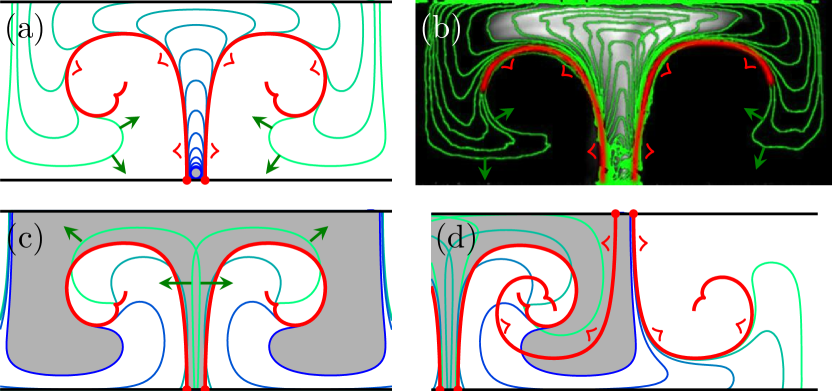
Figure 4: Time-independent flow with reaction fronts ($v_{0}=0.16$). a) BIMs (red) calculated directly from eqs. (1) and (2). Simulation shows reaction front evolving over time (blue to green), converging on the BIMs. b) Experiment shows evolving reaction front (green, images 5 sec apart) and experimentally determined bounding BIMs (red). Each front is extracted from a single reaction image, one of which is shown in white. c) Simulation shows fronts wrapping around the BIM cusp and filling in the vortex centers. Oppositely oriented fronts (green) collide in the image center. d) A neighboring pair of BIMs exists to the right of the original pair. As the front evolves right around the original BIM it encounters the second pair of BIMs, though it is only bounded by the BIM burning in the same direction as the front.

Time-periodic fluid flow, reactive front propagation (fig. 3d): As is the case for the time-independent flow (figs. 3a, c), the addition of reactive burning to the time-periodic flow results in the splitting of each fixed point and their invariant manifolds (figs. 3b, d). The Poincaré map in fig. 3d shows left- and right-burning fixed points, along with left- and right-burning BIMs.

The technique for the extraction of BIMs in the time-periodic case is slightly more complex than in the time-independent case. Each curve in fig. 5a is a snapshot of a simulated evolving front, each of which was catalyzed at a different time in the past but recorded at the common time $t=0$. Thus, although the initial triggering occurs at different phases of the driving, all fronts are imaged at the same phase. This sequence of fronts again converges upon the BIMs (red) which act as local barriers.

Figures 5b-5h show an experimental realization of this protocol. In a series of separate experiments the reaction is triggered at different times $(t<0)$, and therefore different phases of the driving. For each case, the reaction is triggered in a region along the boundary that is mostly between the BIMs, though since the BIMs are close together, the triggered region sometimes overlaps the BIMs. Each reaction is allowed to evolve until it is imaged at $t=0$. The red curves again show the experimentally extracted BIMs . Although eq. (1) is an idealization of the experimental flow, the BIM geometry in the model and experiment is remarkably similar.

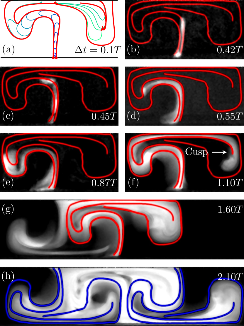
Figure 5: Fronts in time-periodic flow. a) Theoretical model; a front sequence converging onto the BIMs. b) - h) Experimental images of reaction regions (white) and extracted BIMs (red). h) BIMs from the adjacent fixed points are shown in blue. For all panels, $U=0.09$ cm/s, $V_{0}=0.007$ cm/s, $B=0.57$ cm, $\Omega=0.16$ rad/s. Advanced times for trigger are given as multiples of the oscillation period $T=40$ s.

As seen in the time-independent flow, the BIMs form a channel which bounds the sequence of fronts. Upon reaching a cusp singularity in the BIM (fig. 5f), the front sequence wraps around similar to the behavior in the time independent flow (fig. 4). We note that in the model, the cusp is rounded in the opposite orientation (fig. 5a). By perturbing the model parameters, it is possible to alter this orientation. In the next frame (fig. 5g) the reaction moves significantly left of the BIM segment shown. We discuss the details of this mechanism below. After burning beyond the finite BIM segments shown in fig. 5b-g, the reaction front subsequently presses against the neighboring BIMs in fig. 5h (blue) related to the red curves by the flip-shift symmetry of the vortex chain. Their bounding effect on the front propagation is apparent.

As the left BIM in fig. 5f spans the entire channel, it requires some additional explanation to understand how the reaction moves left of this span, since there is no cusp singularity to spiral around, as in fig. 4. The simulation in fig. 6 demonstrates the coevolution of a single reaction front and the left BIM during the course of one complete forcing period. The BIM itself stretches and folds in time, generating a complicated structure that moves both to the left and right. Upon completion of the cycle (fig. 6f), the BIM maps onto itself (original segment in bold). The reaction does not penetrate the BIM (in the burning direction) at any point during this process. Rather, it is the extension of the BIM which allows the reaction to proceed leftward. In fact, the left BIM not only bounds the reacted region, but also draws it along beyond the initial span, and onward down the channel. This process is akin to the canonical turnstile mechanism of passive transport [11].

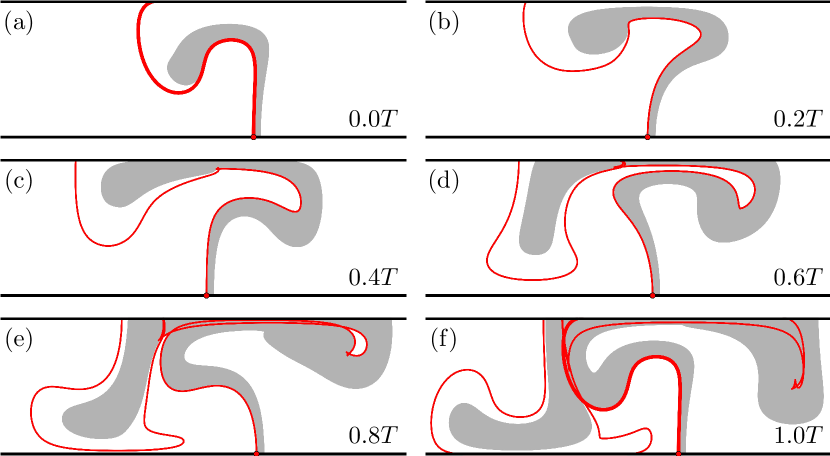
Figure 6: a) A front (gray) begins to the right of the BIM (bold red) in a periodically driven vortex chain flow. A series of snapshots shows the evolution of this particular reaction over one forcing period. The front remains bounded by the evolving BIM at each time. Notice that in (a) the left BIM spans the channel. This sequence shows how the front is able to move beyond the spanning BIM. The original BIM segment is bold in the last frame. Note the good qualitative correspondence of fig. 6a,f with fig. 5d,g.

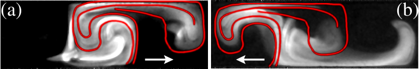
Figure 7: Fronts triggered at generic points to the left a) and right b) of a pair of BIMs. These images illustrate the one-sided nature of the BIMs as barriers.

As noted already for time-independent flows, the BIMs are one-sided barriers; reactions propagating in a direction opposite the BIM’s burning direction pass through unimpeded. Figure 7a shows a front evolving from a generic stimulation point left of the displayed BIMs. The front has burned to the right, through the left-burning BIM, but is bounded by the right-burning BIM. Similarly, a leftward-propagating front passes through a right-burning BIM but is blocked by the left-burning BIM (fig. 7b).

The concepts developed above are robust, since eq. (2) is valid for any 2D incompressible flow, and BIMs are generic features of this ODE. We have observed the presence and influence of BIMs, both experimentally and computationally, for a variety of parameters in the vortex chain. Furthermore, we have demonstrated their existence and function using a spatially disordered, time-independent flow (fig. 8a). As was illustrated for the vortex chain, a reaction triggered near a fixed point in the disordered flow approaches a pair of BIMs, one on either side (fig. 8b). The one-sided nature of the BIMs is also seen in figs. 8c,d; fronts triggered outside the displayed pair of BIMs pass through the BIM encountered first, but stop at the second. Other BIMs observed in this flow share these behaviors.

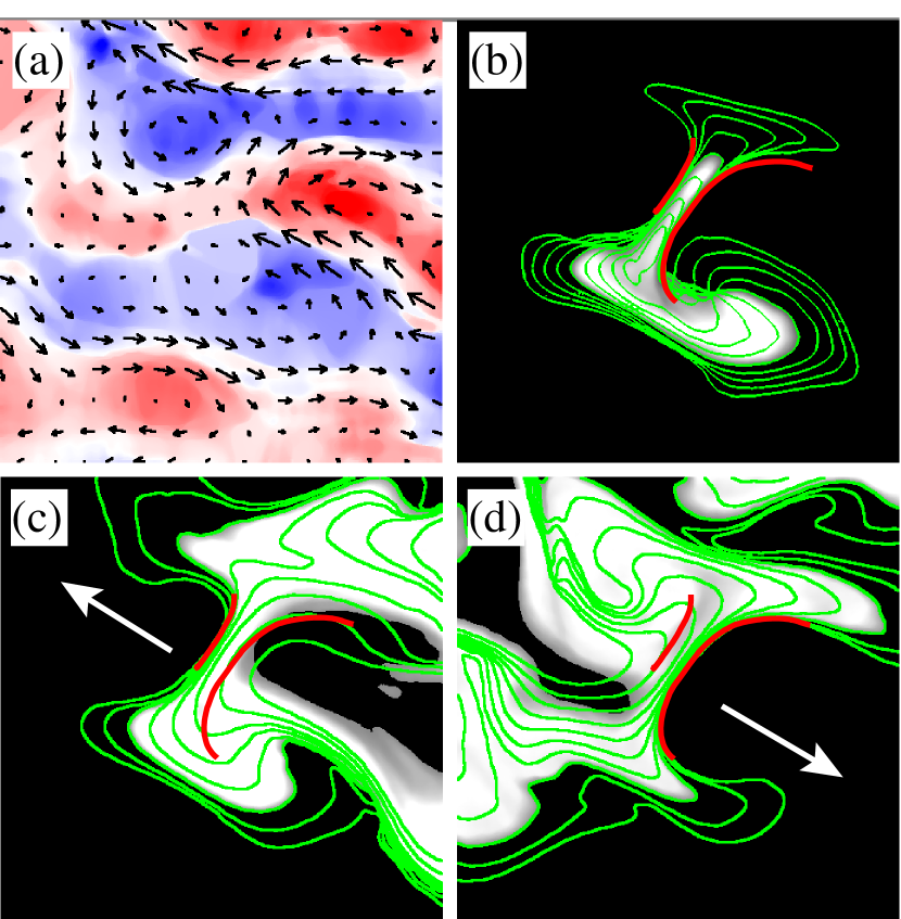
Figure 8: Experiments with 3.55 cm square window of disordered flow. a) Experimental fluid flow measured by particle tracking. Color shows vorticity. b) As in fig. 4b, stimulating between oppositely oriented BIMs produces fronts that approach and are bounded by BIMs. (c, d) Generic stimulations on either side burn through one BIM but not the other.

Summarizing, we have introduced burning invariant manifolds (BIMs) as geometric objects that govern the propagation of reaction fronts in laminar fluid flows. We have shown that BIMs arise naturally from a three-dimensional ODE for reaction front elements, and we have identified BIMs in several experimental flows and have shown that they act as one-sided barriers to front propagation. Currently, we are using BIMs to extend the concept of lobe dynamics [11, 15, 16] to ARD systems. We are investigating the implications of BIM topology for front propagation speeds, providing a necessary alternative to FKPP approaches. We are also developing a method for extracting BIMs in time-aperiodic contexts; this work parallels recent studies of passive transport in which Lagrangian coherent structures [25] were used to extend invariant manifold theory to aperiodic flows.

- [1] \NameTel T., de Moura A., Grebogi C. Karolyi G. \REVIEWPhys. Rep.413200591.
- [2] \NameScotti A. Pineda J. \REVIEWJ. Marine Res.652007117.
- [3] \NameBeule D., Forster A. Fricke T. \REVIEWInt. J. Research Phys. Chem. and Chem. Phys.20419981.
- [4] \NameRussell C. A., Smith D. L., Waller L. A., Childs J. E. Real L. A. \REVIEWProc. Roy. Soc. London Ser. B – Biol. Sci.271200421.
- [5] \NameFisher R. A. \REVIEWAnn. Eugenics71937355.
- [6] \NameKolmogorov A. N., Petrovskii I. G. Piskunov N. S. \REVIEWMoscow Univ. Bull. Math.119371.
- [7] \NameSandulescu M., Lopez C., Hernandez-Garcia E. Feudel U. \REVIEWEcological Complexity52008228.
- [8] \NameJohn T. Mezic I. \REVIEWPhys. Fluids192007.
- [9] \NamePaoletti M. S. Solomon T. H. \REVIEWPhys. Rev. E722005046204.
- [10] \NameOttino J. M. \BookThe Kinematics of Mixing: Stretching, Chaos and Transport (Cambridge University Press, Cambridge) 1989.
- [11] \NameWiggins S. \BookChaotic Transport in Dynamical Systems (Springer-Verlag, New York) 1992.
- [12] \NameSolomon T. H. Gollub J. P. \REVIEWPhys. Rev. A3819886280.
- [13] \NameCamassa R. Wiggins S. \REVIEWPhys. Rev. A431991774.
- [14] \NameSolomon T. H., Tomas S. Warner J. L. \REVIEWPhys. Rev. Lett.7719962682.
- [15] \NameMacKay R. S., Meiss J. D. Percival I. C. \REVIEWPhysica D13198455.
- [16] \NameRom-Kedar V. Wiggins S. \REVIEWArchive for Rational Mechanics and Analysis1091990239.
- [17] \NamePocheau A. Harambat F. \REVIEWPhys. Rev. E732006065304.
- [18] \NameCencini M., Torcini A., Vergni D. Vulpiani A. \REVIEWPhys. Fluids152003679.
- [19] \NameBoehmer J. R. Solomon T. H. \REVIEWEuro. Phys. Lett.83200858002.
- [20] \NameSolomon T. H. Mezić I. \REVIEWNature4252003376.
- [21] \NameAbel M., Celani A., Vergni D. Vulpiani A. \REVIEWPhys. Rev. E642001046307.
- [22] \NameOberlack M. Cheviakov A. F. \REVIEWJ. Eng. Math.662010121.
- [23] \NameNeufeld Z. Hernandez-Garcia E. \BookChemical and Biological Processes in Fluid Flows: A Dynamical Systems Approach (Imperial College Press) 2009.
- [24] \NameYou Z., Kostelich E. J. Yorke J. A. \REVIEWInt. J. Bifurcation Chaos11991605.
- [25] \NameVoth G. A., Haller G. Gollub J. P. \REVIEWPhys. Rev. Lett.882002254501.